Majority Vote Feature Selection Algorithm in Software
Fault Prediction
Emin Borandag1, Akin Ozcift1, Deniz Kilinc1, Fatih Yucalar1
1 Department of Software Engineering, Faculty of Technology, Manisa Celal Bayar University, Manisa, Turkey
{emin.borandag, akin.ozcift, deniz.kilinc, fatih.yucalar}@cbu.edu.tr
Abstract. Identification and location of defects in software projects is an important task to improve software quality and to reduce software test effort estimation cost. In software fault prediction domain, it is known that 20% of the modules will in general contain about 80% of the faults. In order to minimize cost and effort, it is considerably important to identify those most error prone modules precisely and correct them in time. Machine Learning (ML) algorithms are frequently used to locate error prone modules automatically. Furthermore, the performance of the algorithms is closely related to determine the most valuable software metrics. The aim of this research is to develop a Majority Vote based Feature Selection algorithm (MVFS) to identify the most valuable software metrics. The core idea of the method is to identify the most influential software metrics with the collaboration of various feature rankers. To test the efficiency of the proposed method, we used CM1, JM1, KC1, PC1, Eclipse Equinox, Eclipse JDT datasets and J48, NB, K-NN (IBk) ML algorithms. The experiments show that the proposed method is able to find out the most significant software metrics that enhances defect prediction performance.
Keywords: software fault prediction, majority voting, machine learning algorithm
1.
Introduction
software attributes among all. In this context, development of a feature selection model is the main focus of this study [3].
Investigation of relevant metrics is a search problem and the answer to this problem is the exploration of software metric space with the use of feature selection strategies. The feature selection process attempt to locate the feature subsets that represent the data at least as good as the original data with all features. In particular, the feature selection strategies are classified in two groups, i.e. filtering and wrapper feature subset selection algorithms [4]. Filtering based algorithms makes use of some statistical criteria to arrange attributes according to their importance or weights. On the other hand, wrapper methods locate the most predictive feature subset with the use of search algorithms. It is expected that relevant feature subsets may produce a better prediction ability compared to the features alone [5]. In this study, we evaluate filtering based feature selection algorithms to obtain an effective feature subset.
The problem with subset selection is that evaluation of whole candidate metric subsets is ineffective in terms of computational resources. Therefore, we explain our Majority Vote based Feature Selection (MVFS) strategy in having two steps. First we rank the metrics according to their relative importance with the help of 4 well-known feature filtering strategies, i.e. Information Gain (IG), Symmetrical Uncertainty (SU), ReliefF (RLF) and Correlation-based (CO) [6], second, we select the relevant metric subset with a voting scheme borrowed from ensemble learning domain [7]. In this strategy, each feature in the subset is obtained with the majority votes of the feature filtering algorithms on the feature. Having obtained feature subsets with the proposed strategy, we make use of 3 machine learning algorithms i.e. Naïve Bayes (NB), Decision Tree (J48), and K Nearest Neighbor (K-NN/IBk) [8], to evaluate the defect prediction ability of corresponding software metrics. The experimental results show that gradual decrease of software metric space with the proposed MVFS algorithm increases performance of the models.
The main contribution of the study is following: Basic feature filtering strategies are better to be combined in some way to obtain an improved fault prediction performance. In the software fault prediction literature, there are many hybrid strategies that combine feature selection strategies to obtain hybrid methods. To the best of our knowledge, this is the first study that makes use of a voting mechanism to investigate the most relevant features. The remainder of the paper is organized as follows. In section 2, we briefly discuss related work. The evaluation dataset and related information is given in Section 3. In Section 4, we present ranker based filters and the machine learning algorithms used in the study. Section 5 gives details about proposed feature selection algorithm, detailed results of the conducted experiments, and ANOVA test employed for statistically validate the obtained results. In Section 6, validity threats of the study are presented. The article ends with conclusion and as well a list of references.
2.
Related Work
study, one of the most important fields of SBSE searches is related with the obtaining optimum feature model. In other words, a valuable search field in SBSE is to find alternative methods for selecting effective features. In this paper, as an answer to SBSE optimum feature model problem, we propose a hybrid feature selection strategy, i.e. MVFS, to investigate effective software metrics for fault-prediction [9, 10].
There are many feature selection methods used to obtain the most relevant subset of features particularly for improving defect discrimination performance of prediction algorithms [11]. Many studies from literature surveys feature selection strategies and in general feature selection algorithms are classified as filters, wrappers and hybrid methods [12]. Filter based feature methods makes ranking of features from the most relevant to the least relevant with the use of statistical and entropy-based correlation criteria [13]. Chi-square (CS), Gain Ratio (GR), Information Gain (IG), Symmetrical Uncertainty (SU) and ReliefF (RLF) are widely used feature ranker methods [14].
Though filter rankers are classifier independent feature selection methods, wrappers help to obtain relevant feature subset depending on the classification accuracy of a core classifier. The methods search whole feature space adding or removing features to calculate the estimated accuracy of the core classifier. Generally, an exhaustive search is impractical, and therefore non-exhaustive, search methods such as e genetic algorithms, greedy stepwise, best first or random search are often preferred. Since filtering based selection approaches are independent of a classifier they are more efficient from computational cost of view. However, this relative gain is obtained with the loss of awareness of possible dependency between features and the prediction algorithm [15].
The wrapper algorithms propose solution to take account this dependency while obtaining feature subset at the expense of a computational cost. Hybrid feature selection strategies are trade-off solutions for both feature selection domains. They have made combination of multi feature selection approaches to acquire the best feature subset. One particular benefit of hybrid solutions help the use of benefits of filter and wrapper approaches. For instance a combination of filter selection methods is used in [16] to obtain a promising feature subset. The authors have developed a hybrid similarity measure based on defect categories and compare the performance of their metric with IG, GR and RLF on Area Under the Curve (AUC) metric. They have made use of 11 NASA Promise datasets and they have obtained about 70 % better values in terms of number of projects with the use of their hybrid similarity measure in comparison to classical filtering approaches. In an another two-step hybrid feature selection strategy [17], the authors have used CS, SU and RLF to determine relevance of the software metrics in tandem with a clustering strategy to obtain the optimum subset of features from Eclipse and NASA KC1 projects. They have utilized AUC and F-measure metrics to evaluate their results and they have stated that their hybrid methodology has increased the fault prediction performance compared to relevancy measures alone. In the literature, there are many feature selection studies that makes a combination of filter and wrapper approaches in some way to obtain the most valuable feature subset. [18] is an empirical study that investigates value of hybrid feature selection strategies.
building a wrapper model to evaluate a software fault predictor [20]. Jacob et al. propose a hybrid selection method combining information gain ratio and correlation based feature selection applied on NASA datasets [21]. In their detailed empirical work, Catal et al. investigate effects of various feature selection techniques on public datasets from PROMISE repository with the use of RF and NB algorithms [22]. In their recent work [23], the authors use a multivariate linear regression stepwise forward feature selection as a wrapper fashion to obtain optimal set of source code metrics. Another recent work makes use of a hybrid feature selection to improve fault prediction performance of machine learning algorithms [24]. As a last study from literature, Chen et al. improves performance of their machine learning algorithms with two-step hybrid feature selection methodology [25].
There are many studies in the software engineering domain making use of feature selection methods to improve defect prediction accuracies of the algorithms. One of the key points observed in the recent studies is that hybrid of feature selection strategies are preferred to take benefit of multiple extraction techniques at the same time. The rationale behind this approach is similar to ensemble learning methodologies that rely on the performance of ensemble learners rather than a single learner [26]. In this context, hybrid feature selection strategies are continuously explored particularly in software fault prediction domain. Our feature-selection combination strategy, i.e. MVFS, is explained in section 5.1 is an extension to the ongoing search.
3.
Software Measurement Data
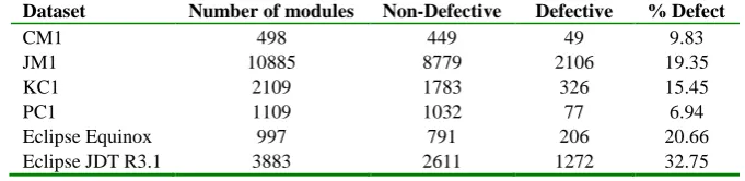
In this study, we have used datasets from PROMISE repository [27], Eclipse Equinox [28] and Eclipse JDT R3.1 [29] bug prediction datasets given in Table 1. First four datasets are from NASA software projects which were developed in C/C++ language for spacecraft instrument, storage management, flight and earth orbiting. Eclipse Equinox Bug Prediction Dataset which was developed in Java language for the infrastructure of the Java IDE. The brief descriptions of the datasets are presented in Table 1.
Table 1. The description of datasets
Dataset Number of modules Non-Defective Defective % Defect
CM1 498 449 49 9.83
JM1 10885 8779 2106 19.35
KC1 2109 1783 326 15.45
PC1 1109 1032 77 6.94
Eclipse Equinox 997 791 206 20.66
Eclipse JDT R3.1 3883 2611 1272 32.75
Table 2. Description of NASA software metrics
Metric type Software metrics Description
McCabe
LOC Line count of code
v(g) Cyclomatic complexity ev(g) Essential complexity iv(g) Design complexity
Derived Halstead
N Total operators + operands
V Volume
L Program length
D Difficulty
I Intelligence
E Effort to write code
B Effort estimate
T Time estimator
Basic Halstead
IOCode Line count
IOComment Comment count IOBlank Blank line count
IOCodeAndComment Number of code and comment lines uniq_Op Number of unique operators uniq_Opnd Number of unique operands
total_Op Number of total operators total_Opnd Number of total operands branchCount Number of branch counts
Class defects Describing whether a software
module is defective or not
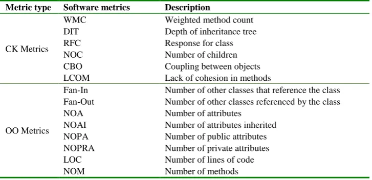
On the other hand, Eclipse Equinox consists of 38 metrics: 6 Chidamber & Kemer (CK) metrics [34], 11 Object-Oriented (OO) metrics [35], 5 entropy metrics [35], 15 change metrics [36, 37], and the last metric is ‘bug’ that describing whether a file is bug or not. The brief description of these metrics is given in Table 3.
Table 3. Description of Eclipse Equinox software metrics Metric type Software metrics Description
CK Metrics
WMC Weighted method count
DIT Depth of inheritance tree
RFC Response for class
NOC Number of children
CBO Coupling between objects
LCOM Lack of cohesion in methods
OO Metrics
Fan-In Number of other classes that reference the class Fan-Out Number of other classes referenced by the class
NOA Number of attributes
NOAI Number of attributes inherited
NOPA Number of public attributes
NOPRA Number of private attributes
LOC Number of lines of code
NOMI Number of methods inherited
NOPM Number of public methods
NOPRM Number of private methods
Entropy Metrics
HCM Entropy of code changes
WHCM Weighted entropy
LDHCM Linearly decayed entropy
LGDHCM Logarithmically decayed entropy
EDHCM Exponentially decayed entropy
Change Metrics
NR Number of revisions of a file
NFIX Number of times file was involved in bug-fixing NREF Number of times file has been refactored NAUTH Number of authors who committed the file LOC_ADDED Sum over all revisions of the LOC added to a file maxLOC_ADDED Maximum number of LOC added for all revisions avgLOC_ADDED Average LOC added per revision
LOC_REMOVED Sum over all revisions of the LOC removed from a file
max LOC_REMOVED Maximum number of LOC removed for all revisions avg LOC_REMOVED Average LOC removed per revision
codeCHU Sum of code churn over all revisions maxCodeCHU Maximum code churn for all revisions avgCodeCHU Average code churn per revision
AGE Age of a file in weeks
WAGE Weighted age
Class Bugs Describing whether a file is bug or not
The features of Eclipse JDT R3.1 dataset is taken from the study Mausa et al. [29].
4.
Majority Vote Feature Selection Algorithm in Software Fault
Prediction
4.1. Feature Filtering Methods
4.1.1. Information Gain
Information Gain (IG) is a widely used feature selection method based on Shannon’s entropy which describes the level of importance between random variable Y and a given information X [38]. In machine learning, IG is used to measure the attribute’s information gain with respect to the class label. This method can be work with both nominal and numerical feature values with an appropriate normalization. IG score of an attribute A can be calculated as follows.
𝐼𝐺(𝐴) = 𝐻(𝑆) − ∑𝑆𝑖 𝑆𝐻(𝑆𝑖) 𝑖
(1)
where H(S) is the total entropy of the dataset and H(Si) is the entropy of the ith subset generated by partitioning S based on feature A.
4.1.2. Symmetrical Uncertainty
Symmetrical Uncertainty (SU) is the normalized form of Information Gain [39] and is calculated with the following equation.
𝑆𝑈(𝑆, 𝐴) = 2 ∗ 𝐼𝐺(𝑆|𝐴)
𝐻(𝑆) + 𝐻(𝐴) (2)
The SU method works similarly to IG. In addition to the score calculated for information gain, it defines the information content of a particular attribute, including definitions of the attribute and the entropy structure of the class.
4.1.3. ReliefF
ReliefF feature selection method measures the importance of an attribute by repeatedly sampling an instance and taking into account the value of the given attribute for its two nearest instances, one instance from the same class, and the other instance from the different class [40]. This method is very effective when working with large amounts of data. Since the number of performed sampling trials is constant, ReliefF feature selection method can run quicker than other methods. The algorithm of ReliefF method for a given m number of sampled instances and k number of features is shown in Figure 1.
Set all weights W[Ai] = 0.0; for j = 1 to m do begin
W[Ai] = W[Ai] – diff(Ai, X, H) / m + diff(Ai, X, M) / m
end; Fig. 1. ReliefF Algorithm
4.1.4. Correlation based approach
Correlation based feature selection approach evaluates the importance of an attribute by measuring the Pearson's correlation between the attribute and the target class [41]. This method simply measures linear correlation between features. The following formula indicates the calculation of Correlation Coefficient (R) between the attribute A and class C.
𝑅(𝑓𝑖, 𝑦) = 𝑐𝑜𝑣(𝑓𝑖, 𝑦)
√𝑣𝑎𝑟(𝑓𝑖) 𝑣𝑎𝑟(𝑦)
(3)
4.2. Machine Learning ClassifiersNaïve Bayes
Naïve Bayes (NB) is a well-known machine learning classifier based on statistical Bayes Theorem and conditional probability [42]. Bayes theorem provides to calculate the posterior probability, P(c | x), from P(c), P(x), and P(x | c). NB classifier presumes that the impact of the value of a feature (x) on a given class (c) is independent of the values of other attributes. This assumption is called class conditional independence and calculated with following equations.
𝑃(𝑐|𝑥) =𝑃(𝑥|𝑐)𝑃(𝑐)
𝑃(𝑥) (4)
𝑃(𝑐|𝑥) = 𝑃(𝑥1|𝑐) ∗ 𝑃(𝑥2|𝑐) ∗ … ∗ 𝑃(𝑥𝑛|𝑐) ∗ 𝑃(𝑐) (5)
where P(c | x) is the posterior probability of class given feature. P(c) is the prior probability of class. P(x | c) is the likelihood which is the probability of feature given class. P(x) is the prior probability of attribute.
4.2.2. Decision Tree
4.2.3. K-Nearest Neighbor
K-Nearest Neighbor (K-NN) is a simple instance-based and lazy learning classification algorithm having no training phase [44]. The distance between the test data and remaining instances is calculated, finally the class having maximum count is selected from the nearest k samples. In K-NN, Euclidean and Cosine similarity measures are the most common algorithms to calculate the distance [45]. In the proposed study, a Weka implementation of K-NN algorithm called IBk is employed.
4.2. Evaluation Criteria
Different criteria are employed to evaluate the performance of classifiers in Machine Learning. All criteria are formulized using a confusion matrix that contains actual and predicted class labels. True Positives (TP), True Negatives (TN), False Positives (FP), and False Negatives (FN) indicates the four different prediction outcomes [46]. In software fault prediction literature, Geometric Mean - 1 (GM) is used by researchers such as Ma et al[46] and Cagatay et al[47] for the valuation of prediction systems to benchmark ML algorithms [48]. In this study, we therefore have used GM to evaluate performance of our algorithms. GM is also a good performance indicator when the datasets are imbalanced and it is used for the evaluation of fault prediction systems [47]. GM metric is calculated using Eq. 6.
Geometric Mean1 = √(𝑝𝑟𝑒𝑐𝑖𝑠𝑖𝑜𝑛 ∗ 𝑟𝑒𝑐𝑎𝑙𝑙) (6)
In 6, Precision is the ratio of correctly predicted positive instances and total predicted positive instances. Furthermore Recall is the defined as the ratio of correctly predicted positive instances and total number of correctly observed positive instances. Precision and Recall are calculated with Eq. 7 and 8 respectively.
𝑃𝑟𝑒𝑐𝑖𝑠𝑖𝑜𝑛 = 𝑇𝑃
𝑇𝑃 + 𝐹𝑃 (7)
𝑅𝑒𝑐𝑎𝑙𝑙 = 𝑇𝑃 𝑇𝑃 + 𝐹𝑁
(8)
5.
Experimental Study and Analysis
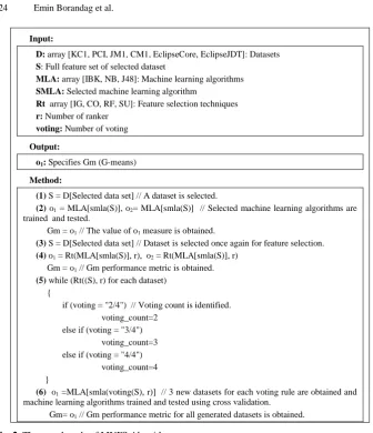
5.1. Design
Input:
D: array [KC1, PCI, JM1, CM1, EclipseCore, EclipseJDT]: Datasets
S: Full feature set of selected dataset
MLA: array [IBK, NB, J48]: Machine learning algorithms
SMLA: Selected machine learning algorithm
Rt array [IG, CO, RF, SU]: Feature selection techniques
r: Number of ranker
voting: Number of voting
Output:
o1: Specifies Gm (G-means)
Method:
(1) S = D[Selected data set] // A dataset is selected.
(2) o1 = MLA[smla(S)], o2= MLA[smla(S)] // Selected machine learning algorithms are
trained and tested.
Gm = o1 // The value of o1 measure is obtained.
(3) S = D[Selected data set] // Dataset is selected once again for feature selection.
(4) o1 = Rt(MLA[smla(S)], r), o2 = Rt(MLA[smla(S)], r)
Gm = o1 // Gm performance metric is obtained.
(5) while (Rt((S), r) for each dataset)
{
if (voting = "2/4") // Voting count is identified. voting_count=2
else if (voting = "3/4") voting_count=3 else if (voting = "4/4")
voting_count=4 }
(6) o1 =MLA[smla(voting(S), r)] // 3 new datasets for each voting rule are obtained and
machine learning algorithms trained and tested using cross validation.
Gm= o1 // Gm performance metric for all generated datasets is obtained.
Fig. 2. The pseudocode of MVFS Algorithm.
In brief terms, the proposed algorithm runs as follows:
NASA and Eclipse projects are used with all features and tested with NB, J48 and IBK algorithms on top of 10-fold cross validation scheme to obtain GM metric. In the second phase IG, CO, RF and SY rankers are used to obtain top 20 software metrics and the experiments are revaluated. In this phase, MVFS algorithm is run using 2/4, 3/4 and 4/4 voting rules and 3 new datasets with reduced features are obtained. The dimensionally reduced datasets are used and GM metric is obtained for NB, J48 and IBK classifiers. This cycle is repeated as follows: (i) obtain subset of features gradually 20, 15, 10, 5 and run MVFS to obtain 3 new data sets for each voting rule, (ii) use 10-CV train-test model for NB, J48 and IBK and obtain GM performance metric for all generated datasets.
continuous variables, any kernel method for prediction of the distribution is not used. The default parameters for IBK and J48 algorithm are also employed in the study. For IBK, the value of parameter k is selected as 1, distance weighting is not applied and Euclidean distance is chosen as distance function.
5.2. Results
In this section, we give details corresponding to the designed algorithm. The overall results corresponding to each project are given in related tables. However, we did not provide the results for all voting rules. We instead selected the best performance metrics for the sake of convenience. Additionally, in order to make interpretation of tables easier and illustrate the performance of the proposed algorithm more obvious, we produced recapping figures for each table.
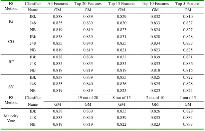
Table 4. Experimental Results for Project KC1 FS
Method
Classifier All Features Top 20 Features Top 15 Features Top 10 Features Top 5 Features
Name GM GM GM GM GM
IG
IBk 0.838 0.839 0.829 0.832 0.810
J48 0.835 0.839 0.830 0.833 0.837
NB 0.819 0.819 0.823 0.824 0.827
CO
IBk 0.838 0.839 0.831 0.828 0.828
J48 0.835 0.840 0.835 0.834 0.833
NB 0.819 0.819 0.821 0.823 0.825
RF
IBk 0.838 0.838 0.832 0.839 0.831
J48 0.835 0.833 0.835 0.833 0.836
NB 0.819 0.819 0.819 0.818 0.816
SY
IBk 0.838 0.839 0.835 0.825 0.822
J48 0.835 0.840 0.836 0.825 0.828
NB 0.819 0.819 0.825 0.823 0.824
FS Method
Classifier 19 out of 20 8 out of 15 2 out of 10 1 out of 5
Name GM GM GM GM GM
Majority Vote
IBk 0.838 0.839 0.833 0.826 0.829
J48 0.835 0.840 0.839 0.835 0.834
NB 0.819 0.819 0.822 0.823 0.837
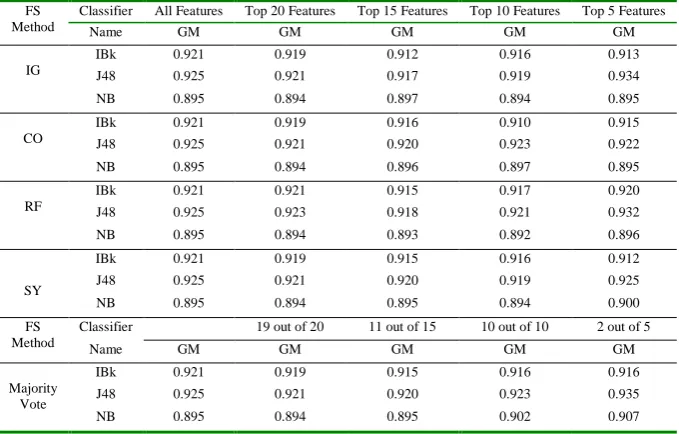
Fig. 3. Illustration of Experimental Results of Table 4 Table 5. Experimental Results for Project PC1
FS Method
Classifier All Features Top 20 Features Top 15 Features Top 10 Features Top 5 Features
Name GM GM GM GM GM
IG
IBk 0.921 0.919 0.912 0.916 0.913
J48 0.925 0.921 0.917 0.919 0.934
NB 0.895 0.894 0.897 0.894 0.895
CO
IBk 0.921 0.919 0.916 0.910 0.915
J48 0.925 0.921 0.920 0.923 0.922
NB 0.895 0.894 0.896 0.897 0.895
RF
IBk 0.921 0.921 0.915 0.917 0.920
J48 0.925 0.923 0.918 0.921 0.932
NB 0.895 0.894 0.893 0.892 0.896
SY
IBk 0.921 0.919 0.915 0.916 0.912
J48 0.925 0.921 0.920 0.919 0.925
NB 0.895 0.894 0.895 0.894 0.900
FS Method
Classifier 19 out of 20 11 out of 15 10 out of 10 2 out of 5
Name GM GM GM GM GM
Majority Vote
IBk 0.921 0.919 0.915 0.916 0.916
J48 0.925 0.921 0.920 0.923 0.935
NB 0.895 0.894 0.895 0.902 0.907
Fig. 4. Illustration of Experimental Results of Table 5
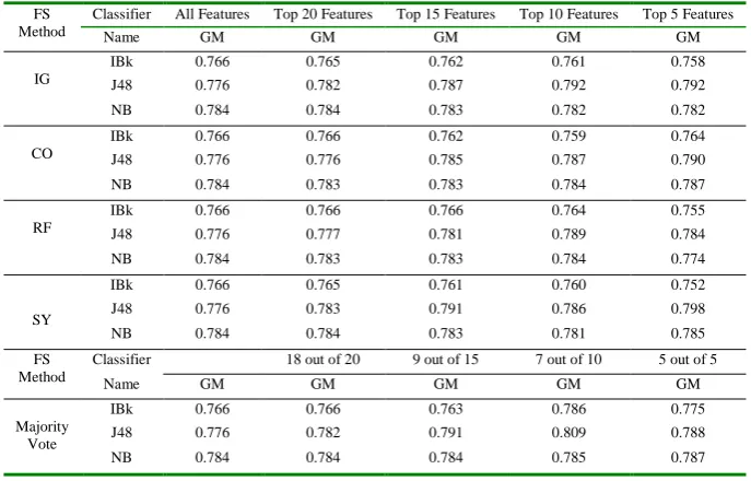
The experiment conducted on Project JM1 is given in Table 6 and the visualization of the results is provided in Figure5.
Table 6. Experimental Results for Project JM1 FS
Method
Classifier All Features Top 20 Features Top 15 Features Top 10 Features Top 5 Features
Name GM GM GM GM GM
IG
IBk 0.766 0.765 0.762 0.761 0.758
J48 0.776 0.782 0.787 0.792 0.792
NB 0.784 0.784 0.783 0.782 0.782
CO
IBk 0.766 0.766 0.762 0.759 0.764
J48 0.776 0.776 0.785 0.787 0.790
NB 0.784 0.783 0.783 0.784 0.787
RF
IBk 0.766 0.766 0.766 0.764 0.755
J48 0.776 0.777 0.781 0.789 0.784
NB 0.784 0.783 0.783 0.784 0.774
SY
IBk 0.766 0.765 0.761 0.760 0.752
J48 0.776 0.783 0.791 0.786 0.798
NB 0.784 0.784 0.783 0.781 0.785
FS Method
Classifier 18 out of 20 9 out of 15 7 out of 10 5 out of 5
Name GM GM GM GM GM
Majority Vote
IBk 0.766 0.766 0.763 0.786 0.775
J48 0.776 0.782 0.791 0.809 0.788
NB 0.784 0.784 0.784 0.785 0.787
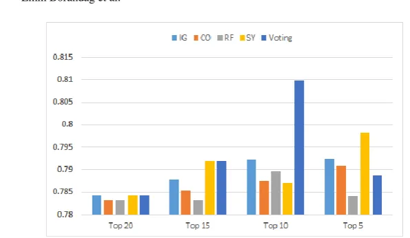
Fig. 5. Illustration of Experimental Results of Table 6
CM1, another NASA projects, is evaluated with the same scheme explained before. The results of the experiments and the corresponding sum up figure is given as Table 7, Figure 6 respectively.
Table 7. Experimental Results for Project CM1 FS
Method
Classifier All Features Top 20 Features Top 15 Features Top 10 Features Top 5 Features
Name GM GM GM GM GM
IG
IBk 0.843 0.843 0.851 0.835 0.848
J48 0.855 0.850 0.851 0.850 0.850
NB 0.857 0.856 0.856 0.862 0.866
CO
IBk 0.843 0.843 0.836 0.837 0.832
J48 0.855 0.855 0.859 0.850 0.851
NB 0.857 0.857 0.855 0.857 0.866
RF
IBk 0.843 0.843 0.838 0.847 0.830
J48 0.855 0.854 0.853 0.845 0.856
NB 0.857 0.857 0.855 0.855 0.855
SY
IBk 0.843 0.843 0.851 0.835 0.840
J48 0.855 0.855 0.851 0.850 0.851
NB 0.857 0.857 0.856 0.862 0.870
FS Method
Classifier 19 out of 20 13 out of 15 9 out of 10 4 out of 5
Name GM GM GM GM GM
Majority Vote
IBk 0.843 0.843 0.848 0.851 0.861
J48 0.855 0.855 0.856 0.850 0.856
NB 0.857 0.857 0.855 0.869 0.872
Fig. 6. Illustration of Experimental Results of Table 7
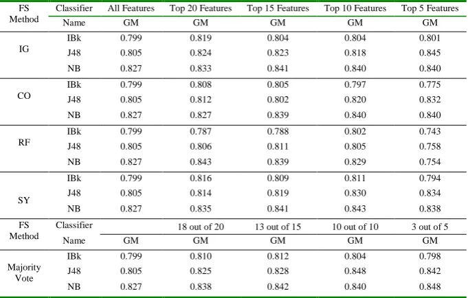
The evaluation results of Eclipse Equinox dataset, is provided in Table 8 and corresponding Figure 7.
Table 8. Experimental Results for Project Eclipse Equinox Core Dataset FS
Method
Classifier All Features Top 20 Features Top 15 Features Top 10 Features Top 5 Features
Name GM GM GM GM GM
IG
IBk 0.799 0.819 0.804 0.804 0.801
J48 0.805 0.824 0.823 0.818 0.845
NB 0.827 0.833 0.841 0.840 0.840
CO
IBk 0.799 0.808 0.805 0.797 0.775
J48 0.805 0.812 0.802 0.820 0.832
NB 0.827 0.827 0.839 0.840 0.840
RF
IBk 0.799 0.787 0.788 0.802 0.743
J48 0.805 0.806 0.811 0.805 0.758
NB 0.827 0.843 0.839 0.829 0.754
SY
IBk 0.799 0.816 0.809 0.811 0.794
J48 0.805 0.814 0.819 0.830 0.834
NB 0.827 0.835 0.841 0.843 0.838
FS Method
Classifier 18 out of 20 13 out of 15 10 out of 10 3 out of 5
Name GM GM GM GM GM
Majority Vote
IBk 0.799 0.810 0.812 0.804 0.798
J48 0.805 0.825 0.828 0.848 0.842
NB 0.827 0.838 0.842 0.840 0.848
Fig. 7. Illustration of Experimental Results of Table 8
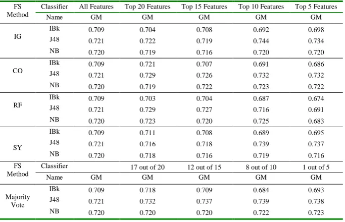
The evaluation results of last dataset, Eclipse JDT dataset, is provided in Table 9 and in the corresponding Figure 8.
Table 9. Experimental Results for Project Eclipse JDT Dataset FS
Method
Classifier All Features Top 20 Features Top 15 Features Top 10 Features Top 5 Features
Name GM GM GM GM GM
IG
IBk 0.709 0.704 0.708 0.692 0.698
J48 0.721 0.722 0.719 0.744 0.734
NB 0.720 0.719 0.716 0.720 0.720
CO
IBk 0.709 0.721 0.707 0.691 0.686
J48 0.721 0.729 0.726 0.732 0.732
NB 0.720 0.719 0.722 0.723 0.722
RF
IBk 0.709 0.703 0.704 0.687 0.674
J48 0.721 0.729 0.727 0.716 0.691
NB 0.720 0.723 0.720 0.725 0.683
SY
IBk 0.709 0.711 0.708 0.689 0.695
J48 0.721 0.716 0.718 0.739 0.737
NB 0.720 0.718 0.716 0.719 0.716
FS Method
Classifier 17 out of 20 12 out of 15 8 out of 10 1 out of 5
Name GM GM GM GM GM
Majority Vote
IBk 0.709 0.718 0.709 0.684 0.693
J48 0.721 0.732 0.737 0.739 0.738
NB 0.720 0.720 0.720 0.722 0.723
Fig. 8. Illustration of Experimental Results of Table 9
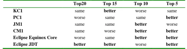
As a sum up of this section, we summarize the results of the experiments and compare the performance of our method with conventional feature rankers based on GM metric in Table 10.
Table 10. Overall Evaluation of Experimental Results based on GM
Top20 Top 15 Top 10 Top 5
KC1 same better worse same
PC1 worse same same better
JM1 same same better worse
CM1 same worse better better
Eclipse Equinox Core worse same better better
Eclipse JDT better better worse better
As the Table 10 is examined, it is seen that the proposed method is eligible to discriminate most valuable software metrics that are functional in software fault prediction detection. Table 10 provides the comparative results of proposed MVFS algorithm and standard rankers, i.e., IG, SU, RF and CO.
For all datasets, MVFS algorithm yields similar results compared to conventional rankers for top 20 and top 15 features. Furthermore, as it can be observed from Table 10, our approach is able to find the most informative software metrics at top 10 or top 5 features. As an overall summary, we may draw a conclusion from Table 10 that the proposed method either increases the prediction of the algorithms or keep their performance as the same.
We have moreover calculated mean and medians of the predictions of the classifiers from the related tables to compare overall results. The results of these statistical calculations are given in Table 11.
Table 11. Median and Mean Calculations of Classier Results based on GM
Top20 Top 15 Top 10 Top 5
KC1
Mean Value 0.839 0.834 0.831 0.834
Median Value 0.839 0.835 0.833 0.834
Majority Value 0.840 0.839 0.835 0.837
Median Base Result better better better better
Mean Base Result better better better better
PC1
Mean Value 0.921 0.918 0.920 0.928
Median Value 0.921 0.919 0.920 0.928
Majority Value 0.921 0.920 0.923 0.935
Median Base Result same better better better
Mean Base Result same better better better
JM1
Mean Value 0.783 0.786 0.788 0.791
Median Value 0.784 0.786 0.788 0.791
Majority Value 0.784 0.791 0.809 0.788
Median Base Result better better better worse Mean Base Result same Better better worse
CM1
Mean Value 0.856 0.856 0.859 0.864
Median Value 0.857 0.856 0.859 0.866
Majority Value 0.857 0.856 0.869 0.872
Median Base Result better same better better
Mean Base Result same same better better
Eclipse Equinox Core
Mean Value 0.834 0.840 0.838 0.820
Median Value 0.834 0.840 0.840 0.839
Majority Value 0.838 0.842 0.848 0.848
Median Base Result better better better better
Mean Base Result better better better better
Eclipse JDT
Mean Value 0.724 0.722 0.735 0.723
Median Value 0.725 0.722 0.735 0.733
Majority Value 0.732 0.737 0.739 0.738
Median Base Result better better better better
Mean Base Result better better better better
5.3. ANOVA Test and Validation
hypothesis regarding the method performed on Minitab statistical software. The statistical values of ANOVA test are given in Figure 9. Parameters of the test, namely, DF, SS, MS, F and p-value correspond to degrees of freedom, adjusted sum of squares, adjusted mean square, F-statistics and probability value, respectively [51].
Fig. 9. Two-way ANOVA test results
Fig. 10. Main Effects Plot for G-means
statistically significant difference between the GM values for feature selection method and classifiers. That is, differences for predictive performance of different feature sets do not exhibit a varying pattern based on the classifiers.
In Figure 10, the main effects plots for classification GM values of the empirical analysis is given. It summarizes comparatively the main findings of the study based on the average results of experiments. As it can be seen from Figure 10, the highest performance in terms of accuracy values were obtained by the proposed majority voting based feature section method. Regarding the performance of classification algorithms, the highest predictive performance (in terms of GM) was achieved by J48 algorithm. Regarding the datasets utilized in the empirical analysis, PC1 dataset yields the highest performance. In Figure 11, the histograms of residuals for all empirical results (in terms of GM) are presented to examine the distribution of empirical results. As it can be observed, the patterns for residuals of all observations exhibit a skewed distribution, which validate the statistical differences obtained by two-way ANOVA test results presented in Figure 11.
Fig. 31. Histogram of Residuals
6.
Threads to Validity
Selection of classifier parameters, being another thread, have also influence on the corresponding results. Even the same classifier with different parameters may affect the related fault-detection performance and therefore selection of the set of classifier parameters are also evaluated in the study.
One more important thread is that the classifier fault-detection performances may vary with the selected subset of metrics. In this context, our proposed method uses a voting ensemble strategy to obtain an optimal set of metrics. The method makes use of a majority combination rule to select the most significant metrics from the results of four different widely used ranker algorithms. Voting based ensembles may also be obtained with averaging or weighting combination mechanisms that may influence the results. Other empirical studies may take advantage of various combinations to obtain the best subset of software metrics [52].
This study makes use of various feature selection algorithms, their ensemble combinations. The quality of the obtained subset of features is evaluated with various classifiers. To reduce modeling errors to minimum, the experiments and statistical investigation were conducted by only one skilled researcher.
7.
Conclusion
Quality in selection of software metrics is critical in the fault detection performance of prediction models. Therefore intelligent selection of software metrics is the first step to obtain an accurate model. We present a collaborative feature selection model to discriminate the most informative software metrics and eliminate other irrelevant metrics. We made use of six software projects and three machine learning algorithms in order to compare performance of or MVFS algorithm with four conventional rankers. As a result, it is empirically observed in the sum up Table 10 that the proposed method is either increases the fault detection performance or retain it as the same compared to the performance of the standard feature selection methods. The obtained experimental results are statistically supported with two-way ANOVA test conducted for GM values. As a future work, we want to test the performance of the proposed MVFS algorithm with the use of another software projects to demonstrate its efficiency.
References
1. Koru, A. G., Liu, H.: Building Effective Defect-Prediction Models in Practice. IEEE Software. 22(6): 23-29. (2005)
2. Azeem, N., Usmani, S.: Defect Prediction Leads to High Quality Product. Journal of Software Engineering and Applications. 4(11): 639-645. (2011)
3. Gao, K., Khoshgoftaar, T. M., Wang, H., Seliya, N.: Choosing software metrics for defect prediction: an investigation on feature selection techniques. Software Practice and Experience. 41(5): 579-606. (2011)
5. Mandal, P., Ami, A. S.: Selecting Best Attributes for Software Defect Prediction. IEEE International WIE Conference on Electrical and Computer Engineering (WIECON-ECE). (2015)
6. Khoshgoftaar, T. M., Gao, K., Napolitano, A.: An Empirical Study of Predictive Modeling Techniques of Software Quality. In: Suzuki J., Nakano T. (eds.) Bio-Inspired Models of Network, Information, and Computing Systems. Lecture Notes of the Institute for Computer Sciences, Social Informatics and Telecommunications Engineering. vol. 87. Springer. Berlin, Heidelberg, pp. 288-302. (2012)
7. Onan, A., Korukoğlu, S., Bulut, H.: A multiobjective weighted voting ensemble classifier based on differential evolution algorithm for text sentiment classification. Expert Systems with Applications. 62(C): 1-16. (2016)
8. Witten, I. H., Frank, E.: Data Mining: Practical Machine Learning Tools and Techniques with Java Implementations. 2nd edition. Morgan Kaufmann. (2005)
9. Harman, M., Jia, Y., Krinke, J., Langdon, W. B., Petke, J., Zhang, Y.: Search based software engineering for software product line engineering: a survey and directions for future work. Proceedings of the 18th International Software Product Line Conference. vol. 1. pp. 5-18. (2014)
10. Shahpar, Z., Khatibi, V., Tanavar, A., Sarikhani, R.: Improvement of effort estimation accuracy in software projects using a feature selection approach. Journal of Advances in Computer Engineering and Technology. 2(4): 31-38. (2016)
11. Chu, C., Hsu, A-L., Chou, K-H., Bandettini, P., Lin, C-P.: Does feature selection improve classification accuracy? Impact of sample size and feature selection on classification using anatomical magnetic resonance images. NeuroImage. 60(1): 59-70. (2012)
12. Jović, A., Brkić, K., Bogunović, N.: Review of feature selection methods with applications. 38th International Convention on Information and Communication Technology. Electronics and Microelectronics (MIPRO). (2015)
13. Guyon, I., Elisseeff, A.: An Introduction to Variable and Feature Selection. Journal of Machine Learning Research. vol. 3. pp. 1157-1182. (2003).
14. Novaković, J., Strbac, P., Bulatović, D.: Toward Optimal Feature Selection Using Ranking Methods and Classification Algorithms. Yugoslav Journal of Operations Research. 21(1): 119-135. (2011).
15. Janecek, A. G. K., Gansterer, W. N., Demel, M. A., Ecker, G. F.: On the Relationship between Feature Selection and Classification Accuracy. Proceedings of the 2008 International Conference on New Challenges for Feature Selection in Data Mining and Knowledge Discovery. vol. 4. pp. 90-105. (2008)
16. YU .Q., JIANG S., WANG R., WANG H. : A feature selection approach based on a similarity measure for software defect prediction. Frontiers of Information Technology & Electronic Engineering. pp. 1744-1753 (2017)
17. Chen J., Liu S., Chen X., Gu Q., Chen D. Empirical Studies on Feature Selection for Software FaultPrediction, 5th Asia-Pacific Symposium on Internetware, (2013)
18. Afzal, W., Torkar, R.: Towards Benchmarking Feature Subset Selection Methods for Software Fault Prediction. Computational Intelligence and Quantitative Software Engineering, pp. 33-58. (2016)
19. Wang, H., Khoshgoftaar, T. M., Seliya, N.: How Many Software Metrics Should be Selected for Defect Prediction?. Proceedings of the Twenty-Fourth International Florida Artificial Intelligence Research Society Conference. Palm Beach, Florida, USA. (2011) 20. Soleimani, A., Asdaghi, F.: An AIS based feature selection method for software fault
21. Jacob, S., Raju, G.: Software Defect Prediction in Large Space Systems through Hybrid Feature Selection and Classification. The International Arab Journal of Information Technology, 14(2): 208-214. (2017)
22. Catal, C., Diri, B.: Investigating the effect of dataset size, metrics sets, and feature selection techniques on software fault prediction problem, Information Sciences, 179(8): 1040-1058. (2009)
23. Kumar, L., Rath, S., Sureka, A.: Using Source Code Metrics and Ensemble Methods for Fault Proneness Prediction. https://arxiv.org/abs/1704.04383, (2017)
24. Alighardashi, F., Chahooki, M. A. Z.: The Effectiveness of the Fused Weighted Filter Feature Selection Method to Improve Software Fault Prediction. Journal of Communications Technology. Electronics and Computer Science. vol. 8. pp. 5-11. (2016) 25. Chen, J., Liu, S., Chen, X., Gu, Q., Chen, D.: Empirical Studies on Feature Selection for
Software Fault Prediction. Proceedings of the 5th Asia-Pacific Symposium on Internetware. (2013)
26. Dietterich, T. G.: Ensemble Methods in Machine Learning. In: Multiple Classifier Systems. Lecture Notes in Computer Science. vol. 1857. Springer, Berlin, Heidelberg, pp. 1-15. (2000)
27. Software Defect Dataset, Promise Repository. January (2018). [Online]. Available: http://promise.site.uottawa.ca/SERepository/datasets-page.html
28. Eclipse Bug Prediction Dataset. Eclipse Equinox. January (2018). [Online]. Available: http://bug.inf.usi.ch/data/eclipse.zip
29. Mauša G., Grbac T. G., Bašić B. D., A Systematic Data Collection Procedure for Software Defect Prediction, ComSIS Consortium vol 13, Issue 1 , (2016)
30. McCabe, T. J.: A complexity measure. IEEE Transactions on Software Engineering. 2(4): 308–320. (1976)
31. Halstead, M. H.: Elements of software science. Elsevier Computer Science Library. Operating and Programming Systems Series. New York, Oxford, (1977)
32. Tutorial on McCabe and Halsted. January (2018). [Online]. Available: http://openscience.us/repo/defect/mccabehalsted/tut.html
33. Rodriguez, D., Ruiz, R., Gallego, J. C., Aguilar-Ruiz, J.: Detecting Fault Modules Applying Feature Selection to Classifiers. IEEE International Conference on Information Reuse and Integration. (2007)
34. Basili, V. R., Briand, L. C., Melo, W. L.: A Validation of Object-Oriented Design Metrics as Quality Indicators. IEEE Transactions on Software Engineering. 22(10): 751-761. (1996) 35. D’Ambros, M., Lanza, M., Robbes, R.: An Extensive Comparison of Bug Prediction
Approaches. 7th IEEE Working Conference on Mining Software Repositories. IEEE CS Press. pp. 31-41. (2010)
36. Moser, R., Pedrycz, W., Succi, G.: A comparative analysis of the efficiency of change metrics and static code attributes for defect prediction. Proceedings of the 30th International Conference on Software Engineering. pp. 181–190. (2008)
37. Muthukumaran, K., Bhanu Murthy, N. L.: Impact of Restricted Forward Greedy Feature Selection Technique on Bug Prediction. PeerJ Computer Science. (2015)
38. Yang, Y., Pedersen, J. O.: A comparative study on feature selection in text categorization. Proceedings of the 14th International Conference on Machine Learning (ICML '97). Nashville, Tenn, USA. Morgan Kaufmann. pp. 412–420. (1997)
40. Kononenko, I.: Estimating Attributes: Analysis and Extensions of RELIEF. In: Proceedings of the 7th European Conference on Machine Learning, pp. 171–182. (1994)
41. Hall, M. A., Smith, L. A.: Feature selection for machine learning: comparing a correlation-based filter approach to the wrapper. Proceedings of the Twelfth International Florida Artificial Intelligence Research Society Conference. pp. 235-239. (1999)
42. Pedregosa, F., Varoquaux, G., Gramfort, A., Michel, V., Thirion, B., Grisel, O., Blondel, M., Prettenhofer, P., Weiss, R., Dubourg, V., Vanderplas, J.: Scikit-learn: Machine learning in Python. Journal of Machine Learning Research. vol. 12. pp. 2825-2830. (2011)
43. Khoshgoftaar, T. M., Seliya, N.: Tree-based software quality estimation models for fault prediction. Eighth IEEE Symposium on Software Metrics. pp. 203-214. (2002)
44. Aha, D. W., Kibler, D., Albert, M. K.: Instance-based Learning Algorithms. Machine Learning. 6(1): 37-66. (1991)
45. Qian, G., Sural, S., Gu, Y., Pramanik, S.: Similarity between Euclidean and cosine angle distance for nearest neighbor queries. Proceedings of the 2004 ACM symposium on applied computing. pp. 1232-1237. (2004)
46. Ma Y., Guo L., Cukic B., A Statistical Framework for the Prediction of Fault-Proneness, Advances in Machine Learning Application in Software Engineering, Idea Group Inc., pp. 237-265, (2006)
47. Catal C., Performance Evaluation Metrics for Software Fault Prediction Studies, Acta Polytechnica Hungarica vol. 9, no. 4, (2012)
48. Y. Ma, L. Guo, B. Cukic, A Statistical Framework for the Prediction of Fault-Proneness, Advances in Machine Learning Application in Software Engineering, Idea Group Inc., 2006, pp. 237-265
49. Witten IH., Frank E., Data Mining: Practical Machine Learning Tools and Techniques. San Francisco, CA: Morgan Kaufman, (2005)
50. Amancio DR., Comin CH., Casanova D.,Travieso G.,Bruno OM.,Rodrigues FA.,Costa L., A systematic comparison of supervised classifiers. PloS one; 9(4): pp. 94-137 (2014). 51. Onan, A., Korukoglu, S., Bulut, H.: Ensemble of keyword extraction methods and
classifiers in text classification. Expert Systems with Applications. 57(C): 232–247. (2016) 52. Polikar R., Ensemble Based Systems in Decision Making IEEE Circuits And Systems
Magazinepp 21-45 (2006).
Emin Borandag is currently working as an Assistant Professor in the Department of Software Engineering, Manisa Celal Bayar University, Manisa, Turkey. He received BS and MS degrees in computer engineering from Maltepe University in 2003 and 2006, respectively. He was awarded PhD in computer engineering from Trakya University in 2011. His research interests are the area of software quality assurance, software testing and data mining.
Deniz Kilinc is currently working as an Assoc Professor in the Department of Software Engineering, Celal Bayar University, Manisa, Turkey. He received BS and MS degrees in computer engineering from Dokuz Eylül University in 2002 and 2004, respectively. He was awarded PhD in computer engineering from Dokuz Eylül University in 2010. His research interests focus on information retrieval, software engineering, text mining and social media
analysis.
Fatih Yücalar is currently working as an Assistant Professor in the Department of Software Engineering, Manisa Celal Bayar University, Manisa, Turkey. He received BS and MS degrees in computer engineering from Maltepe University in 2002 and 2006, respectively. He was awarded PhD in computer engineering from Trakya University in 2011. His research interests focus on software engineering, software project management, software quality assurance and testing.