Classification Credit Dataset Using Particle Swarm Optimization and Probabilistic Neural Network Models Based on the Dynamic Decay Learning Algorithm

(1)

Published online September 20, 2013 (http://www.sciencepublishinggroup.com/j/acis) doi: 10.11648/j.acis.20130105.12

Classification credit dataset using particle swarm

optimization and probabilistic neural network models

based on the dynamic decay learning algorithm

Reza Narimani

1, *

, Ahmad Narimani

2

1

Department of Financial Engineering, University of Economic Sciences, Tehran, Iran

2

Department of Economics, University of AllamehTabatabae'i, Tehran, Iran

Email addresses:

[email protected] (R. Narimani), [email protected] (A. Narimani)

To cite this article:

Reza Narimani, Ahmad Narimani. Classification Credit Dataset Using Particle Swarm Optimization and Probabilistic Neural Network Models Based on the Dynamic Decay Learning Algorithm. Automation, Control and Intelligent Systems. Vol. 1, No. 5, 2013, pp. 103-112. doi:10.11648/j.acis.20130105.12

Abstract:

This paper describes a credit risk evaluation system that uses supervised probabilistic neural network (PNN) models based on the Dynamic Decay learning algorithm (DDA). The PNN-DDA has two parameters called positive and negative threshold. This learning algorithm trains very quickly. Thus it makes sense that we use a meta-heuristic algorithm such as particle swarm optimization to optimize these parameters. When using the meta-heuristic algorithm such PSO, the tuning process of parameters is implemented wisely. Thus in this paper we also obtained optimum threshold. Two credit datasets in UCI database are selected as the experimental data to demonstrate the accuracy of the proposed model. The result shows that this new hybrid algorithm outperforms the most common used algorithm such as multi-layer neural network.

Keywords:

Probabilistic Neural Network Particle Swarm Optimization, Dynamic Decay Algorithm, Classification

1. Introduction and Related Work

One another of first studies that became well-known in credit risk measurement was Z-score that is obtained from multi variable scoring model (Altman, 1968). This model is multiple discriminant analysis (MDA) that by using important financial ratios tries to distinguish between bankrupt and non-bankrupt firms. With attention to this fact that most unpaid loan are related to the firms that will have financial distress in future, so credit risk prediction is possible by this model. In this way, Saunders and Allen, 2002, used this model for credit risk of the firms that borrowed loan from banks. Their investigation showed that MDA has high performance of prediction capability.

In the context of credit risk measurement, we can mention another important study was conducted by the work of Elmer and Borowski, 1988. They predict loan repayment ability by multi-layer perceptron neural network model. Their input variables ware the same as the variables used in the model Z-Altman model. They compared the results from neural network model and the z-Altman model

and found that the capability of credit scoring prediction of neural network is higher than the z-Altman model. Among the studies that were conducted in the area of credit risk measurement model, Morgan, 1998 work on designing a credit risk model can be mentioned.

Traditional statistical methods such as linear

discriminant models (Reichert, Cho, & Wagner, 1983), logit and probit models (Beaver, 1966 and Ohlson, 1980 & Henley, 1995) in the past two decades were the most applicable models but the use of models based on neural networks increased the accuracy of these predictions significantly.

(2)

Han & Kwon, 1996; Boritz and Kennedy, 1995), and classification and regression trees (Davis, Edelman, & Gammerman, 1992), and Support Vector Machines (SVMs) (Min and Lee, 2005; Shin and Lee & Kim, 2005), and genetic algorithm (Shin and Lee, 2002; Varetto, 1998) are used.

Artificial neural networks (ANN) are one of the strongest data mining tasks which can be used for finding the nonlinear nature and pattern of data. They are inspired by the biological network of neurons in the human brain (Mira & Sanchez-Andres, 1999).

Hsieh, 2005, present a hybrid approach based on clustering and neural network techniques. They used clustering techniques to preprocess the input samples with the objective of indicating unrepresentative samples into isolated and inconsistent clusters, and used neural networks to construct the credit scoring model.

Khashman, 2010, described a credit risk evaluation system that uses supervised neural network models based on the back propagation learning algorithm. In this paper, the dataset used for evaluation was German credit. So the input layer size was 24, but they use three neural networks with 18, 23 and 27 hidden layer size respectively.

Hybrid model have more flexibility that can mimic the nonlinearity of behavior of data relationships. These models don’t have the limits of traditional classification models.

The researchers use PNN model for pattern recognition context such as: marketing (Kazemi, 2013), signal processing (Übeyli, 2008), medical/biochemical field applications (Mantzaris, 2011; Hajmeer, 2002), civil (Tam, 2004).

The most interesting algorithms in PNN and RBS neural network is Dynamic Decay learning algorithm (DDA) (Berthold and Diamond,1995; Berthold and Diamond, 1998).

RBFN-DDA is a dynamically growing neural network that adapts the numbers of neurons to the data space. The main difference of RBFN-DDA to the PNN is the smaller number of utilized neurons in the hidden layer.

While PNN uses one hidden neuron for one available sample, i.e., a kind of memorizing every sample, RBFN-DDA generalizes the data by only inserting a neuron in the network when it becomes necessary (Paetz, 2002)

Topouzelis and Karathanassi & Pavlakis & Rokos, 2004 compared Radial Basis Function (RBF) neural network trained by Dynamic Decay learning algorithm (DDA) and multi-layer neural network to in oil spill detection. The results showed that MLPs appear to be superior to RBFs in detecting oil spills on Synthetic Aperture Radar (SAR) images.

Our purpose of this paper is to introduce the hybrid algorithm to enhance the learning of RBF neural network by DDA.

2. Probabilistic Neural Network (PNN)

Probabilistic neural networks are a special type of feed-forward neural networks that are based on radial basis functions that using Bayes' decision theory to classify input pattern (Donal F.Specht 1988; Donal F.Specht 1991). By doing some modification on RBF neural networks, it is possible to estimate probability density function (PDF) of each class pattern.

Probabilistic neural networks are a form of normalized Radial-Basis Form (RBF) neural networks, where each hidden node is a “kernel” implementing a probability density function (Jones, 2008).

So PNN has three layer fixed structure as RBF. A PNN is a four-layer architecture which consists of input, pattern, summation and output layers (Ding, X., Yeh, C.-H., & Bedingfield, S, 2010). The pattern and summation layer consist the hidden layer. Probabilistic neural network architecture is shown in Figure 1.

+ ‐

+

+ ‐ ‐

Output layer

Summation layer

Pattern layer

Input layer

d 2 1,X,...,X

X   

 

  

 

      

 −

−

= ∑

=

d

1 i

2

ij ij i j

σ x x exp A

∑

=

= n

1 j

j

A n 1 f(x)

Figure 1. Probabilistic neural network architecture

So PNN includes an input layer, a hidden layer and an output layer. Input layer has the responsibility of distribution and it does not implement any process in it. All neurons in the hidden layer have the activation function of radial basis functions usually are selected in the form of Gaussian type. The neurons in the hidden layer receive input vectors and have two parameters: 1) center 2) spread.

Amount of overlap between adjacent neurons in hidden layer neurons determine this spread. Each hidden layer neuron can be said to be simply has larger output when the input vector is closer to the center of the non-linear function of neurons. With increasing the distance of input vector from the center of non-linear functions, the output of neurons is also reduced.

The output layer is a competitive layer. The number of neurons in competitive layer is equal to the number of classes. Activation function of the hidden layer is as follows:

        ₋

=

ij ij i j ij

x x a

σ

ψ (1)

(3)

of the hidden layer.

σ

_ij, x_ij and a_ijare spread, center and output of jth neuron of hidden layer respectively.

Output of jth neuron of hidden layer

( )

A_j is obtained by the product of the activation functions that is as follows:

        ₋ ∏ = ∏ = = = _ij ij i j d i ij d i j x x a A σ ψ 1 1 (2)

Where d is the number of dimensions in the input vector. If the activation function

( )

ψ is selected in the form of the Gaussian:                   ₋ − = 2 exp ij ij i x x σ ψ (3)

Eq 2 became as follows:

                  ₋ − = ∏ =

∑

= = d i ij ij i ij d i j x x a A 1 2 1 exp σ (4)

But the main part of the training of PNN is based on the probabilistic technique that is implemented by using of Bayes strategy and Parzen’s non-parametric estimation technique. By using Bayes' decision theory and satisfying following equation, learning sample can be assigned to the category k.

) ( )

(x h l f x f

l

h_k _k _k > _q_q _q ₍₅₎

k

h and h_q respectively are prior probability for the class k and q; The probability that sample had been selected from class k or q. lkand lqare probability of classification

error. On the other hand, Parzen showed that if the kernel function concentrates on some part of a class of samples then it is a good approximation of probability density function for that class. Probability density function for a class can be approximated by the following formula:

(

)

∑

=                ₋ ₋               = k n j kj k d d k x x n x pdf 1 2 2 2 2 exp 0 . 1 2 0 . 1 ) ( σ σ

π (6)

The value ofn_kis equal to the number of data in class k, and d is the number of dimensions in the input vector. x_kj

represents the center of the Gaussian function and is corresponding to the jth sample in the dataset belonging to the class k.

This seemingly complicated formula meaning that at first, the summation of Gaussian functions is calculated then the average of them is gained and then multiplied by weighting factor (the first sentence in the relationship), including fixed terms and nth power of spread. Clearly, the choice of σ has an important effect onpdf_k(x). If σ is too large, the estimate will suffer from too little resolution; if σ is too small, the estimate will suffer from too much statistical

variability (Duda, 2001). One way to reach the optimum σ is try and error method.

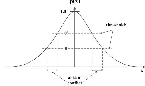
This algorithm introduces the idea of distinguishing between matching and conflicting neighbors in an area of conflict. Two different thresholds: θ+ and θ− as illustrated in Figure 2.

p(x) thresholds area of conflict 1.0 x

Figure 2. Two different thresholds: θ+ and θ−in PNN trained by DDA algorithm

They are used to define intersection of influencing area.

+

θ determines the minimum correct classification

probability for training patterns of the correct class. In contrast θ−is used to avoid misclassifications; that is the probability for an incorrect class for each training pattern is less than or equal to θ−(M. Berthold, J. Diamond 1998).

In general the DDA algorithm comprises the following three steps (Chiang Tan, 2006):

• Covered. If a new pattern is correctly classified by an already existing prototype, it initiates regional expansion of the winning prototype in the attribute space.

• Commit. If a node of the correct class does not cover a new pattern, a new hidden node will be introduced, and the new pattern is codded as reference vector.

• Shrink. If a new pattern is incorrectly classified by an already existing prototype of conflicting classes, the width of conflicting classes, the width of the prototype will be reduced (i.e. shrunk) for the sake of overcoming the conflict.

These steps are shown in Table 1 and Figure 3.

Table 1. Dynamic Decay learning algorithm (DDA)

FORALL prototypes p_ikDO // reset weights 0 . 0 = k i A ENDFOR

FORALL training pattern(x,c)DO: // train one complete epoch

(4)

add new neuron c_m

c

p ₊₁with: // commit new neuron

x r_mc

c+1=

; ln min

2 1

1 c

1

mc −

+

≤ ≤≠ +

− − =

θ σ

c m k j

m j c k

c

s

r r

0 . 1 =

c mc

A

1 = +

c

m

ENDIF

FORALL k≠c, 1≤j≤m_kDO // shrink radius of

conflicting neurons

; ln , min

2 k

j

     

     

− −

= ₋

θ σ

σ

k j k

j

r x

ENDFOR

where pci = i-the neurons of class c (c∈{1,…,n}, n classes),

+ c

θ

,

θ

c− : controlling size of overlapping regions of

neurons in respect to each class, m is the number of _c

neurons for class c, r_ic is the center of neuronsp_ic,

σ

_icis the radius of neuronpc_i .

(a)

(b)

(c)

(d)

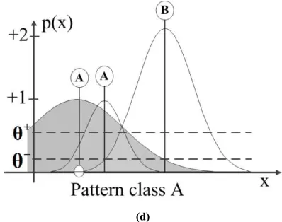
Figure 3. The procedure of applying thresholds on data: (a) a pattern of class A is encountered and a new RBF is created (b) a training pattern of class B leads to a new prototype for class B and shrinks the radius of the existing RBF of class A (c) another pattern of class B is classified correctly and shrinks again the prototype of class A (d) a new pattern of class A introduces another prototype of that class.

3. Particle Swarm Optimization (PSO)

Algorithm

Originally, particle swarm optimization was proposed by Kennedy and Eberhart (1995). The main idea of PSO is to mimic social behavior of birds. In PSO algorithm, each particle can move along the linear combination of its personal velocity, towards best global position and towards best local of its personal position in the problem space. The velocity of a particle is updated according to Eqs. 7 and 8.

(

() ()

)

( () ()), )

( ) 1

(t wv t r1C1P t x t r2C2 g t x t

vij + = ij + ij − ij + j − ij (7)

), 1 ( ) ( ) 1

(t+ =x t +v t+

x_i_j _ij _i_j ₍₈₎

where w is inertia weight that shows the effect of previous velocity on new velocity vector. C1 and C2 are positive

constant, r1 and r2 are random variables with uniform

distribution in between 0 and 1.

4. Empirical Analysis

Credit data Sets

(5)

Table 2. Basic information of the two credit datasets

No. 1 2

Names German Australian

# classes 2 2

# instances 1000 690

Nominal features 0 6

Numeric

features 24 8

Total

features 24 14

No. of good instances 700 307

No. of bad instances 300 383

5. Performance Evaluation Criteria

The fundamental issue for rating a classifier’s performance is the confusion matrix where the numbers represent the total number of actual classes and predicted classes. (Hassan and Ramamohanarao and Karmakar and Hossain & Bailey, 2010)

A confusion matrix has shown in Table 3.

Table 3. Confusion matrix

Based on the elements in the confusion matrix, following statistics are defined:

FN TP

TP y sensitivit or

TPR

+

= (9)

FPR FN

TP TN y

specificit = −

+

= 1 (10)

FN TN FP TP

TN TP accuracy

tion classifica

+ + +

+

= (11)

6. Area under the ROC Curve

Sensitivity and specificity rely on a single cut-point to classify a test result as positive. A more complete description of classification accuracy is given by the area under the ROC (Receiver Operating Characteristic) (Hosmer and Lemeshow, 1989).

The vertical axis of an ROC curve represents TPR. The

horizontal axis represents FPR. On the graph, we move right and plot a point. This process is repeated for each of the test tuples in ranked order, each time moving up on the graph for a true positive or toward the right for a false positive (Han and Kamber & Pei, 2012).

The AUC as the fitness function, in the discrete case, can compute with step functions:

− +

= = >

∑ ∑

+ −

− +

=

n n AUC

n

i n

j f xi f xj

1 11 ( ) ( ) ₍₁₂₎

Where f(0)is denoted as the scoring function. x+and

−

x _{respectively denote the positive and negative samples}

and n+and n−are respectively the number of positive and negative examples and 1 is defined to be 1 if the predicate _π

π holds and 0 otherwise (Campbell & Ying 2011; Rakotomamonjy 2004).

7. Fitness Function

There are three common functions to candidate for fitness function in classification problem:

1. Classification accuracy

2. Specificity × sensitivity

3. Area Under ROC

We use Area Under ROC (AUC) as fitness function in PNN-DDA trained by PSO.

8. A Hybrid Algorithm of PSO and

PNN-DDA

A PSO algorithm using 5-fold cross-validation is carried out on each training set to find the optimal parameter pair

(

_θ+_,_θ−

)

_{. Then, the related dataset is trained with the} obtained optimal parameter pair

(

θ+,θ−

)

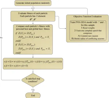
to get a predictor model. This process is shown on Figure 4:

The parameter used in PSO algorithm is shown on Table 4.

Table 4. The parameter used in PSO

Parameter Value

Max number of generations 20

Population size 15

inertia weight (w) 0.7298

C1 1.4962

C2 1.4962

9. Results

(6)

( ) ( )

i ibest

ibest i ibest i

i gbest

gbest i gbest i

if Z X Z P

Z P Z X and P X

endif

if Z X Z P

Z P Z X and P X

endif <

= =

<

= =

1 1 2 2

( 1) ( ) ( ( ) ( )) ( ( ) ( ))

( 1) ( ) ( 1)

i i ibest i gbest i

i i i

v t w v t r c P t x t r c P t x t

x t x t v t

+ = + − + −

+ = + +

−

+_θ

θ ,

Figure 4. A hybrid algorithms that PSO optimize the two parameters (θ+,θ−) in PNN-DDA model

Table 5. classification accuracy results of models

Model

Classification Accuracy (%)

70-30% training-test 80-20% training-test

German Australia German Australia

train test train test train test train test

ANN 0.6614 0.6400 0.8758 0.8599 0.6975 0.7150 0.8696 0.8188

PSO-PNN 0.8386 0.7533 0.9006 0.8599 0.8738 0.7350 0.9130 0.8841

Table 6. AUC results of models

Model

Area Under ROC curve (%)

German Australia German Australia train test train test train test train test

ANN

0.8091 0.7522 0.9430 0.9133 0.8134 0.7920 0.9497 0.9167

PSO-PNN

0.9317 0.7860 0.9632 0.9200 0.9258 0.7664 0.9660 0.9209

(7)

Table 7. Sensitivity, Specificity for two credit data

Model

Sensitivity, Specificity for two credit data

70-30% training-test 80-20% training-test German Australia German Australia train test train test train test train test

ANN Threshold= 0.5

[0.9128 0.4928]

[0.8841 0.4624]

[0.8727 0.9028]

[0.8017 0.9011]

[0.8681 0.5858]

[0.8345 0.5738]

[0.8656 0.9150]

[0.7949 0.9000]

PSO-PNN Threshold=0.5

[0.6714 0.9614]

[0.5749 0.7742]

[0.9625 0.7963]

[0.9397 0.6923]

[0.5882 0.9707]

[0.5036 0.8361]

[0.9475 0.8219]

[0.9487 0.7000]

ANN Optimum Threshold

[0.5842 0.8454]

[0.5749 0.7849]

[0.8127 0.9537]

[0.7845 0.9560]

[0.6595 0.7866]

[0.6906 0.7705]

[0.8098 0.9433]

[0.7436 0.9167]

PSO-PNN Optimum Threshold

[0.8377 0.8406]

[0.7874 0.6774]

[0.8989 0.9028]

[0.8793 0.8352]

[0.8414 0.8452]

[0.7626 0.6721]

[0.9115 0.9150]

[0.8846 0.8833]

The best parameter pairs (

θ

+,

θ

−) of two dataset on each training-test partition are presented in detail in Table 8.

Table 8. The optimal parameters for two credit dataset

Parameters

German Australia German Australia

+

θ 0.8071 0.6109 0.6365 0.6509

−

θ 0.2693 0.2998 0.2608 0.2998

Optimum threshold 0.5488 0.3488 0.5705 0.3998

ANN

Optimum neuron 4 4 2 5

Optimum threshold 0.2515 0.3417 0.3302 0.2535

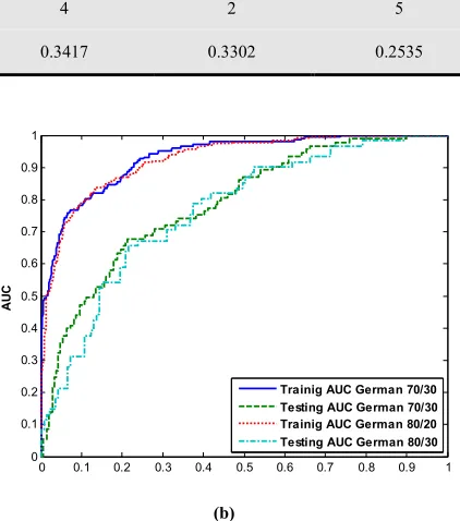
Plotting of ROC curves for the two credit data have shown in Figure 5. The bigger area means better classifier performance.

0 0.1 0.2 0.3 0.4 0.5 0.6 0.7 0.8 0.9 1

A

U

C

Trainig AUC Australian 70/30 Testing AUC Australian 70/30 Trainig AUC Australian 80/20 Testing AUC Australian 80/30

(a)

0 0.1 0.2 0.3 0.4 0.5 0.6 0.7 0.8 0.9 1

A

U

C

Trainig AUC German 70/30 Testing AUC German 70/30 Trainig AUC German 80/20 Testing AUC German 80/30

(b)

(8)

0 50 100 150 200 250 300 350

0.78 0.781 0.782 0.783 0.784

Function Evaluation

A

U

C

o

f

5

-f

o

ld

C

ro

s

-v

a

li

d

a

ti

o

n

0 50 100 150 200 250 300 350

0.752 0.754 0.756 0.758 0.76

German 70/30 German 80/20

(a)

0 50 100 150 200 250 300 350

0.894 0.896 0.898 0.9

Function Evaluation

A

U

C

o

f

5

-f

o

ld

C

ro

s

-v

a

li

d

a

ti

o

n

0 50 100 150 200 250 300 350

0.8995 0.9 0.9005 0.901

Australian 70/30 Australian 80/20

(b)

Figure 6. PSO plot for the best fitness during the training phase on the (a) German and (b) Australian credit dataset

It can be observed that in Figure 6.a, the fitness curves gradually improved from 1 to 230 function evaluations and exhibited no significant improvements after that and in Figure 6.b, the fitness curves gradually improved from 1 to 100 function evaluations and exhibited no significant improvements after that. Eventually the optimization stopped at the 350 function evaluations where the generations reached the stopping criterion.

Hence, this hybrid model can converge quickly to global optima and we can enhance its effectiveness for our hybrid model.

10. Conclusion

We have proposed a new effective approach for two class problems in data mining area by applying the PSO algorithm to optimize the two parameter of PNN-DDA. Achieved results show that the proposed model is worthwhile, since it had a reasonable accuracy on two datasets. Furthermore we calculated the best threshold for

achieving the best ROC curve. According to the values of classification accuracy, it can be realized that the PSO-PNN has the better performance rather than ANN in two dataset and different training-testing partition. Furthermore, PSO-PNN has considerable performance due to the AUC measure.

References

[1] Altman, E. I. (1968). FINANCIAL RATIOS, DISCRIMINANT ANALYSIS AND THE PREDICTION OF CORPORATE BANKRUPTCY. The Journal of Finance, 23, 589-609.

[2] Beaver, W. H. (1966). Financial Ratios As Predictors of Failure. Journal of Accounting Research, 4, 71-111. [3] Berthold, M. R., & Diamond, J. (1998). Constructive

training of probabilistic neural networks. Neurocomputing, 19, pp. 167-183.

[4] Campbell, C & Ying, Y 2011, 'Learning with Support Vector Machines', in SYNTHESIS LECTURES ON ARTIFICIAL INTELLIGENCE AND MACHINE, Morgan and cLaypool. [5] Charalambous, C., Charitou, A., & Kaourou, F. (2000).

Comparative Analysis of Artificial Neural Network Models: Application in Bankruptcy Prediction. Annals of Operations Research, 99, 403-425.

[6] Chiang Tan, S., Rao, M. V. C., & Lim, C. (2006). An Adaptive Fuzzy Min-Max Conflict-Resolving Classifier. In A. Abraham, B. de Baets, M. Köppen & B. Nickolay (Eds.), Applied Soft Computing Technologies: The Challenge of Complexity (Vol. 34, pp. 65-76): Springer Berlin Heidelberg. [7] Davis, R. H., Edelman, D. B., & Gammerman, A. J. (1992).

Machine learning algorithms for credit-card applications. Journal of Mathematics Applied in Business and Industry, 4, 43–51.

[8] Desai, V. S., Crook, J. N., & Overstreet Jr, G. A. (1996). A comparison of neural networks and linear scoring models in the credit union environment. European Journal of Operational Research, 95, 24-37.

[9] Ding, X., Yeh, C.-H., & Bedingfield, S. (2010). A Probabilistic Neural Network Approach to Modeling the Impact of Tobacco Control Policies by Gender. In Z. Zeng & J. Wang (Eds.), Advances in Neural Network Research and Applications (Vol. 67, pp. 869-876): Springer Berlin Heidelberg.

[10] Duda, R. O., Hart, P. E., & Stork, D. G. (2001). Pattern classification. New York: Wiley.

[11] Efrim Boritz, J., & Kennedy, D. B. (1995). Effectiveness of neural network types for prediction of business failure. Expert Systems with Applications, 9, 503-512.

[12] Elmer, Peter J., and David M. Borowski. (1988). An Expert System and Neural Networks Approach To Financial Analysis, Financial Management, No 12, 66-76.

(9)

[14] Han, J., Kamber, M., & Pei, J. (2012). Data mining concepts and techniques, third edition. In. Waltham, Mass.: Morgan Kaufmann Publishers.

[15] Hassan, M. R., Ramamohanarao, K., Karmakar, C., Hossain, M. M., & Bailey, J. (2010). A Novel Scalable Multi-class ROC for Effective Visualization and Computation. In M. Zaki, J. Yu, B. Ravindran & V. Pudi (Eds.), Advances in Knowledge Discovery and Data Mining (Vol. 6118, pp. 107-120): Springer Berlin Heidelberg.

[16] Henley, W. E. (1995). Statistical aspects of credit scoring. Dissertation, The Open University, Milton Keynes, UK. [17] Henley, W. E., & Hand, D. J. (1996). A k-nearest-neighbor

classifier for assessing consumer credit risk. Journal of the Royal Statistical Society Series D: The Statistician, 45, 77-95.

[18] Hosmer, D. W., & Lemeshow, S. (2004). Applied logistic regression. Chichester: Wiley

[19] Hsieh, N. C. (2005). Hybrid mining approach in the design of credit scoring models. Expert Systems with Applications, 28, 655-665.

[20] Huang, C. L., Chen, M. C., & Wang, C. J. (2007). Credit scoring with a data mining approach based on support vector machines. Expert Systems with Applications, 33, 847-856.

[21] J.P. Morgan (April, 1998), Creditmetrics – Technical Document, New York, J.P. Morgan & Co. Incorporated. [22] Jones, M. T. (2008). Artificial intelligence : a systems

approach. Hingham, Mass.: Infinity Science Press.

[23] Kazemi, S. M. R., Hadavandi, E., Mehmanpazir, F., & Nakhostin, M. M. (2013). A hybrid intelligent approach for modeling brand choice and constructing a market response simulator. Knowledge-Based Systems, 40, 101-110. [24] Kennedy, J. and Eberhart, R. (1995). Particle swarm

optimization, Proceeding. IEEE International Conference on Neural Networks (ICNN), Nov./Dec., Australia, Pages 1942–1948.

[25] Khashman, A. (2010). Neural networks for credit risk evaluation: Investigation of different neural models and learning schemes. Expert Systems with Applications, 37, 6233-6239.

[26] Lee, J. J., Kim, D., Chang, S. K., & Nocete, C. F. M. (2009). An improved application technique of the adaptive probabilistic neural network for predicting concrete strength. Computational Materials Science, 44, 988-998.

[27] Lee, K. C., Han, I., & Kwon, Y. (1996). Hybrid neural network models for bankruptcy predictions. Decision Support Systems, 18, 63-72.

[28] M. Berthold, J. Diamond, “Boosting the Performance of RBF Networks with Dynamic Decay Adjustment”, Proc. of the Advances in Neural Information Processing Systems (NIPS), Denver, USA, vol. 7, pp. 521-528, 1995.

[29] Malhotra, R., & Malhotra, D. K. (2002). Differentiating between good credits and bad credits using neuro-fuzzy systems. European Journal of Operational Research, 136, 190-211.

[30] Mantzaris, D., Anastassopoulos, G., & Adamopoulos, A.

(2011). Genetic algorithm pruning of probabilistic neural networks in medical disease estimation. Neural Networks, 24, 831-835.

[31] Min, J. H., & Lee, Y. C. (2005). Bankruptcy prediction using support vector machine with optimal choice of kernel function parameters. Expert Systems with Applications, 28, 603-614.

[32] Mira, J., Sánchez-Andrés, J. V., Engineering Applications of Bio-Inspired Artificial Neural Networks. Alicante, Spain, vol. 2, 1999.

[33] Murphy, P. M., Aha, D. W. (2001). UCI repository of machine learning databases. Department of Information and Computer Science, University of California Irvine, CA.

Available from http://www.ics.

uci.edu/mlearn/MLRepository.htmlurlhttp://www.ics.uci.edu /mlearn/MLRepository.html.

[34] Ohlson, & James, A. (1980). Financial Ratios and the Probabilistic Prediction of Bankruptcy. Journal of Accounting Research, 18, 109.

[35] Paetz, J. (2002). Feature selection for RBF networks. In Neural Information Processing, 2002. ICONIP '02. Proceedings of the 9th International Conference on (Vol. 2, pp. 986-990 vol.982).

[36] Rakotomamonjy, A. (2004). Optimizing area under ROC curves with SVMs. In Proceedings of the ECAI-2004 Workshop on ROC Analysis in AI.

[37] Reichert, A. K., Cho, C.-C., & Wagner, G. M. (1983). An Examination of the Conceptual Issues Involved in Developing Credit-Scoring Models. Journal of Business & Economic Statistics, 1, 101-114.

[38] Saunders, A., Allen, L., & Saunders, A. (2002). Credit risk measurement in and out of the financial crisis: new approaches to value at risk and other paradigms. New York: John Wiley and Sons, 2nd edition.

[39] Shin, K. S., & Lee, Y. J. (2002). A genetic algorithm application in bankruptcy prediction modeling. Expert Systems with Applications, 23, 321-328.

[40] Shin, K. S., Lee, T. S., & Kim, H. J. (2005). An application of support vector machines in bankruptcy prediction model. Expert Systems with Applications, 28, 127-135.

[41] Specht, D. F. (1988). Probabilistic neural networks for classification, mapping, or associative memory. In Neural Networks, 1988., IEEE International Conference on (pp. 525-532 vol.521).

[42] Specht, D. F. (1991). A general regression neural network. Neural Networks, IEEE Transactions on, 2, 568-576. [43] Tam, C. M., Tong, T. K. L., Lau, T. C. T., & Chan, K. K.

(2004). Diagnosis of prestressed concrete pile defects using probabilistic neural networks. Engineering Structures, 26, 1155-1162.

[44] Topouzelis K., V. Karathanassi, P. Pavlakis, D. Rokos, 2004. Oil spill detection using RBF Neural Networks and SAR data, XXth ISPRS Congress, Istanbul, Turkey, July 2004 [45] Übeyli, E. D. (2008). Implementing eigenvector

(10)

[46] Varetto, F. (1998). Genetic algorithms applications in the analysis of insolvency risk. Journal of Banking and Finance, 22, 1421-1439.