JAM: A Tabu-based Two-Stage Simulated
Annealing Algorithm for the Multidimensional
Arrangement Problem
⋆Jordi Arjona Aroca1 and Antonio Fern´andez Anta2
1
Universidad Carlos III de Madrid, Madrid, Spain 2 IMDEA Networks Institute, Madrid, Spain
Abstract. In this paper we study a version of the Multidimensional Arrangement Problem (MAP) that embeds a graph into a multidimen-sional array minimizing the aggregated (Manhattan) distance of the em-bedded edges. This problem includes the minimum Linear Arrangement Problem (minLA) as a special case, among others. We propose JAM, a tabu-based two-stage simulated annealing heuristic for this problem. Our algorithm relies on existing techniques for the minimum linear ar-rangement (minLA) problem, which are non-trivially adapted to work in multiple dimensions. Due to the scarcity of specific benchmarks for MAP, we have tested the performance of our algorithm with benchmarks for the minLA and Quadratic Assignment Problems (with more than 80 graphs). For each graph in these benchmarks, we provide results for 1, 2 and 3-dimensional instances of MAP, enlarging, hence, the benchmark-ing resources for the research community. The results obtained show the practicality of JAM, often matching the best known result and even im-proving some of them.
Keywords: Multidimensional Arrangement Problem, Minimum Linear Arrangement Problem, Quadratic Assignment Problem, Simulated An-nealing, Tabu Search.
1 Introduction
Assignment and arrangement problems have been extensively studied for decades. The most classical and well known application of these prob-lems is the assignment of nfacilities tom locations in order to minimize or maximize a certain magnitude, such as cost, flow, etc. In this work, we deal with one of these arrangement problems, the Multidimensional Arrangement Problem (MAP), which was firstly studied by Hansen [12].
⋆
MAP covers a great number of applications, such as graph drawing or job scheduling (in 1 dimension), the backboard wiring problem or the ar-rangement of electronic components in printed circuits (in 2 dimensions), and placing servers in the racks of a data center (in 3 dimensions).
In this paper we focus on the MAP problem, which embeds a graph into a multidimensional array minimizing the aggregated Manhattan dis-tance. To solve this problem, we propose a hybrid simulated annealing heuristic, non-trivially adapting techniques used for the Minimum Linear Arrangement Problem (minLA, the one-dimensional version of MAP) to work in multiple dimensions.
1.1 Problem Definition
Given a graphG= (V, E) and a hostD-dimensional arrayH(V′, E′) such that |V′| ≥ |V|, we can define the Multidimensional Arrangement Problem as the embedding ofG intoH, i.e., a mapping of the edges of
G to paths in H, such that the aggregated length of the paths in H is minimized. As we will usually work with weighted graphs, the goal is to minimize the weighted sum of the path lengths. Formally, the cost of an embedding φ:V →V′ is defined as
C(φ) = ∑ (u,v)∈E
wuv·dist(φ(u), φ(v)), (1)
where wuv is the weight of edge (u, v) and dist(φ(u), φ(v)) is the Man-hattan distance (the path length) between the images of u and v in the host graph H.
The particular case of D = 1 is a well known problem, called the
minimum linear arrangement (minLA). In this problem, the ob-jective is to embed a graph onto a one dimensional array. As minLA is known to be NP-complete and MAP has minLA as a special case, it can be concluded that MAP is NP-hard.
1.2 Related Work
The Quadratic Assignment Problem, which is a more general problem than MAP, is an NP-hard problem [31] which has been creating inter-est during more than 50 years [16]. The QAP objective function can be mathematically formulated as follows
n ∑
i=1 n ∑
j=1
fij ·dist(π(i)π(j)) + ∑
i,π(i)
wherefij is the flow between facilitiesiandj,π(·) is the location at which a facility has been assigned,dist(x, y) denotes the distance between two locations x and y, and b(i, x) is the initial allocation cost of facility i
to location x. Many well-known problems, like the traveling salesman problem (TSP), minLA, and MAP, are special cases of QAP.
Some exact algorithms have been developed to solve the QAP prob-lem. However, they are only capable to solve small instances due to the enormous computation capacity required. The largest instances solved op-timally surpassed just recently the 100 locations frontier [9], but most of the latest works still work with instances of 30-40 locations [9][26]. These algorithms typically use branch and bound, branch and cut, or dynamic programming.
Approximate methods have also been developed to tackle the QAP problem. We classify them in heuristics and metaheuristics. Starting with heuristics, most of the ones that have been developed can be grouped in constructive, enumeration, and improvement methods. We can find some examples of heuristics applied to the QAP problem in [20, 25, 11].
Despite of the richness in heuristics, metaheuristics have been at-tracting most of the attention lately. Most of the metaheuristics applied to the QAP problem can be included in one of the following families: genetic algorithms (GA) [22, 8], simulated annealing (SA) [4, 38], ant colony optimization (ACO) [32], tabu search (TS) [23, 24, 33, 13], break-out local search (BLS) [2], greedy randomized adaptive search procedures (GRASP) [17], variable neighborhood search (VNS) [39], or hybrid com-binations of them [10, 34]. Given that QAP is more general than MAP, it is possible to adapt many of these techniques to obtain solutions also for MAP.
accept φl as the new φ∗ or refuse it. If a new solution is chosen and it is better than the best-so-far solutionφbest, it becomes the newφbest. After running a given number of iterations the system’s temperature is cooled down. This process follows until a total number of iterations is run or a termination criteria is met.
Observe that the acceptance function allows the heuristic to admit solutions which are worse than the previous ones. This is generally known as climbing up and helps to avoid that heuristics are trapped in a local optimum. Although the mechanics of SA are not complicated, choosing the cooling rate, stop criteria, and neighborhood function is not trivial.
Simulated annealing was one of the first techniques applied to the QAP problem (c.f., Burkard et al. [4], Wilhelm et al. [38]). We now de-scribe some of the main characteristics of some of the latest works using SA, alone or combined with other techniques. We start with the work of Wang [36], who proposed in 2007 a tabu-based simulated annealing algo-rithm. In that work, a pure SA algorithm was compared to a tabu-search SA, trying different tabu list sizes and also trying different guided restart and reannealing strategies, enhancing the ability to escape from local op-tima. In 2012, Wang [37] presented a new work based also on simulated annealing, but trying different guided restart strategies. In both works a local-search-based neighborhood function was used jointly with a geo-metrical cooling rate schedule (like Kirkpatrick et al. [15]), reheating the algorithm when a restart takes place. In 2012, Jingwei et al. [14] presented a new hybrid algorithm combining ant colonies and simulating anneal-ing. Here, simulated annealing was used to select the best ants in each iteration, while the cooling schedule was also geometrical. In 2003, Mis-eviˇcius [21] presented a very detailed work comparing multiple previously proposed cooling schedules. With this, he proposed an SA heuristic using a normal-local-search-based neighborhood function, an inhomogeneus an-nealing cooling schedule without equilibrium tests, like the one proposed by Connolly et al. in [7], and modified reannealing so the cooling schedule oscillates depending on the behavior of the annealing. This heuristic was completed by a post optimization stage based on Taillard’s robust tabu search. This heuristic was even able to improve one of the QAPLIB [3] instances.
minimization algorithm, and the second stage is devoted to improve this initial solution. They consider a modified median-based neighborhood function in which the typical 2-exchange strategy is conditioned by the nodes connected to a candidate-to-be-moved node. They also consider different ways of establishing the initial temperature, based on [35], and a different cooling schedule [1]. We will detail these aspects when describ-ing our algorithm in Section 2, as we adopted and adapted some of their ideas for our MAP heuristic.
1.3 Contributions
In this work we present JAM, a tabu-based two-stage simulated annealing heuristic for MAP. In JAM, we use a novel median-based neighborhood function and we non-trivially adapt multiple techniques from the minLA literature to work for multiple dimensions.
Due to the lack of benchmarks specific for the MAP problem, we test our heuristic against minLA and QAP benchmarks, with weighted and unweighted graphs. The minLA benchmark has a one-dimensional array as host graph, while the QAP benchmarks have a 2-dimensional array as host graph. JAM obtains the optimal or best known result in most of the problem instances. Although the benchmarks used were originally for 1 or 2 dimensions, we present results for them for 1, 2 and 3 dimensions, broadening hence the available benchmarks for minLA and QAP as well as creating a benchmark set for MAP. We also present 2 different results for 2 dimensions. The first one is restricted to the case in which guest and host graphs have the same size, i.e., where |V′|=|V|. The second one is for a deployment which is more compact (square) and that allows having extra locations, i.e., where |V′| ≥ |V|.
RoadMap The paper is organized as follows. In Section 2 we present our own algorithm as well as a detailed description of its different elements. In Section 3 we present the numerical results obtained with our heuristic for multiple benchmarks from the minLA and QAP literature and for which we provide results in 1, 2 and 3 dimensions. We close the paper by presenting some conclusions in Section 4.
2 The Algorithm JAM
Algorithm 1:JAM Pseudo Code
1 φ∗←SetInitialSolution(); 2 φbest←φ∗;
3 k←0;T(k)←SetInitialTemperature(); 4 whilethe termination criteria do not hold do
5 forthe predefined number of iterations at temperatureT(k)do 6 Choose a nodeuuniformly at random;
7 withprobabilitypN: setL←Nu;
8 elsesetL← {l}, wherelis a location chosen uniformly at random; 9 Discard all locationsl∈Lthat would lead to a move in the tabu list; 10 Φ← {φl:φlis the arrangement after movingutolinφ∗,∀l∈L};
11 φ′←arg minφ∈Φ{C(φ)};
12 if C(φ′)> C(φ∗)then
13 φ′←φchosen fromΦwith probability proportional toC(φ); 14 δ←C(φ′)−C(φ∗);
15 withprobabilitye−δ/T(k):φ∗←φ′;φbest←arg min{C(φbest), C(φ∗)};
16 k←k+ 1;T(k)←UpdateTemperature(T(k−1)); 17 GuidedRestart(φ∗,φbest);
2.1 Notation
Given a graphG= (V, E),V and E denote its sets of vertices and edges, respectively. Each edge (i, j) ∈ E has an associated weight denoted by
wij. We denote byAu the set of nodes adjacent to node uin G.
The host graphH(V′, E′) is aD-dimensional array. Recall that|V′| ≥
|V|. The nodes of H are called locations. Each location l∈V′ is defined by a D-vector (l1, l2, . . . , lD), where li is the dimension i coordinate of location l. On the other hand, di(X) is used to denote the dimension i coordinate of all elements of a set X of locations.
In order to improve the costC(φ) of an arrangementφ, JAM performs node “movements.” By movement we refer to the action of “moving” node
ufrom a locationlto a locationl′, and “moving” the nodev, if any, which is at location l′ tol. Formally, this means transforming the arrangement
φinto a new φ′ such thatφ′(x) =φ(x) for all x∈V \ {u, v},φ′(u) =l′, and φ′(v) = l. There is only a set of valid locations to which a node u
can move (see Section 2.3 below), this set is called its neighborhood and is denotedNu.
2.2 Overview of JAM
McAllister heuristic [18]. This arrangement is also the initial best known solution. The current solution and the best known solution are stored inφ∗ and φbest, respectively (Lines 1−2). Then, the initial temperature
T(0) (Line 3) for the SA is computed. After that, the cooling down process starts, which will take place until the termination criteria are met (Line 4). For every temperatureT(k), JAM runs a predefined number of iterations (Line 5), starting with T(0). In each iteration, a node u to be moved is chosen uniformly at random (Line 6). Then, with probability pN, the set of locationsLto whichumay be moved is chosen to be the neighborhood
Nu (Line 7). Otherwise the only location that will be considered is a randomly chosen onel(Line 8). Not explicitly shown in Algorithm 1, JAM maintains a tabu list of movements that are not to be redone. Hence, all elements inLthat lead to a move in this tabu list are discarded (Line 9). Now, the arrangementsΦresulting of movinguto the remaining locations inLare obtained (Line 10), and the arrangementφ′ with the lowest cost among them is chosen (Line 11). If the cost of thisφ′is larger than the cost of the current solutionφ∗,φ′ is replaced by an arrangement chosen from
Φwith probabilities proportional to their respective costs (Line 12−13). To complete the iteration, the proposed φ′ is adopted with probability
e−δ/T(k), which implies updating φ∗ and, if corresponds, φ
best (Line 15). (Observe that ifδ <0 thenφ′ is always adopted.) Once the given number of iterations forT(k) is reached, it is updated (Line 16) and it is decided whether resettingφ∗ toφbest is needed (Line 17).
2.3 Elements of JAM
We now provide a detailed description of the elements mentioned above that conform JAM.
First Stage: Initial Solution McAllister heuristic [18] has been adapted to multiple dimensions and used to obtain an initial solution. McAllister’s is a greedy heuristic based on a frontal increase minimization strategy. It chooses a starting node at random and maps it to some location. Then, it greedily maps the rest of nodes. To do so, it maintains three sets of nodes U (Unplaced), P (Placed) and F (Front, the set of placed nodes with at least one neighbor in set U). The next node to be mapped is the one with the least neighbors in setU \F, so the front set is minimized.
the first node to location (0,0, . . . ,0) in the host graph, and then greed-ily decides which of the neighboring locations to those of the already allocated nodes is the best position, in terms of cost, for the next node.
Initial Temperature We decided to initialize the temperature using the same method as Tello et al. [28], which employs the technique proposed by Varanelli and Cohoon [35]. This method approximates the simulated annealing temperature T(k) at which a solutionφ∗ with costC(φ∗) can be found as best solution. Hence the initial temperature is given by3
T(0)≈ σ 2
∞
C∞−C(φ∗)−γ∞σ∞
,
where C∞ and σ∞ represent the expected cost and average deviation of the cost over the solution space; C(φ∗) represents the cost of the initial solution and γ∞ represents the difference between the expected cost C∞
and the best known solutionφbestat temperatureT(k).γ∞can be calcu-lated probabilistically from the number of iterations predefined at each temperature. We refer the reader to [35] for further details.
Cooling Schedule Our cooling schedule is based on the work from Aarts and Korst [1]. They propose a statistical cooling schedule which depends on the previous temperature, the average deviation of the solutions ob-tained with the previous temperature σT(k−1), and a tuning parameterλ (such that for small values ofλwe obtain small temperature reductions). The cooling schedule is given by the following equation:
T(k) =T(k−1) (
1 +log (1 +λ)T(k−1) 3σT(k−1)
)−1
.
Neighboring Solutions In order to reduce the search space of locations to which a certain nodeucan be moved, we define a median-based neigh-borhood function. This function returns a set of neighbors Nu, which is the set of contiguous locations that will be considered for the movement of
u. Intuitively, we choose the setNu to be the locations that minimize the cost of the edges incident in u assuming that only u changes its location (in this fictitious arrangement u may share location with other nodes).
We describe now the process we use to obtain Nu. Let us assume that the nodes adjacent to u in G are Au = {v1, v2, . . . , vn}, and that
3
their respective current location is lj =φ∗(vj),∀j∈[1, n]. Let us fix one dimension i∈[1, D], and let us sort the nodes in Au by the dimension i
coordinate of their current location, so that lj1
i ≤l j2
i ≤ · · · ≤ l jn
i . Then, we compute the smallest m∈[1, n] that satisfies
∆(m) = m ∑
k=1
wuvjk −
n ∑
k=m+1
wuvjk ≥0.
If∆(m) = 0 then we define a range of valuesri= [ljm, ljm+1). Otherwise, if∆(m)>0 then we define the range as the singleton valueri= [ljm].
After applying this method to each dimension separately we have ranges r1, r2, . . . , rD. The D-polytope obtained by the combination of these ranges is the set of locations in Nu. I.e., all locations l such that
li ∈ ri,∀i ∈ [1, D] belong to Nu. In our implementation of JAM we extended Nu with all the locations that are within distance 2 of the set described, just to increase the movement options.
Evaluating Solutions We defined the cost of an arrangement C(φ) in Eq. 1. However, two different solutions might have the same cost. To consider these cases, we use instead a cost function C′(φ) introduced in [29]. The authors there proposed a refined method for estimating the cost of solutions in a minLA problem which considers not only the cost derived from the paths in H but also how the costs of these paths are distributed. The cost of an arrangementφis then given by
C′(φ) = Θ ∑
k=1 (
k+ n! (n+k)!
)
ek, (2)
where Θ = ∑Di=1di−1 is the diameter of H and ek is the number of paths of length k in H. Note that the second term of this formula is always smaller than 1. Then, for solutions where the cost would be the same if we had only considered the first term, the total cost will be smaller if the arrangement has longer paths. A solution with a larger number of longer paths is preferred as it would be, in principle, easier to improve.
Tabu Search (TS) In order to favor the exploration abilities of JAM we incorporate TS. As we said, moving a nodeu from positionl to position
l′ implies moving the node v in position l′, if any, to position l. Our TS mechanism will check that neither u norv have been in locations l orl′, respectively, during the last Ts moves, being Ts the size of our tabu list.
which that move was done. If a proposed move has been done during the lastTs iterations, it is discarded. There is one exception to this rule, the
aspiration criterion. We implemented the most common one: a move will be accepted, despite of being tabu, when it leads to a smallerC′(φbest).
Guided Restarts We implement guided restarts in order to help the algorithm to escape from some strong local minima. A restart consists in resetting φ∗ to φbest. We decide if a restart is needed after finishing all the iterations at a certain temperature. A restart occurs with probability
P(restart) = 1−e(−
|φ∗−φbest|
φbest T(0) T(k)γ),
whereT(0) andT(k) are the initial and current temperatures, andγ is a tuning parameter that depends on the size of the graph.
Termination Criteria We use two termination criteria. Our algorithm will stop when (1) T(k) goes below a predefined temperature threshold
Tth or when (2) the percentage of accepted moves improving φ∗ while at temperature T(k) goes below a second predefined threshold Pth. The values for these thresholds depend on the size of the graph.
3 Evaluation of JAM
In this section we present the results obtained for a set of benchmark instances ran in order to evaluate JAM’s performance. Ideally, we would have used a set of instances for which we had results in multiple di-mensions. However, due to non-existence, to the best of our knowledge, of such a set of instances, we used graphs belonging to benchmarks from the minLA and QAP literature. Our intention, however, is two-fold. First, we want to create such a collection of instances so they can be used in future MAP works as benchmark. Second, by running these graphs in 1 and 2 dimensions, we are broadening the available number of instances and results for both minLA and QAP benchmark collections.
Table 2 and for the first results in 2 dimensions in Table 3. For the 3-dimensional host graphs we chose the number of nodes in each dimension so that the number of empty locations is minimized. In these tables R,
C and D denote the number of nodes in the respective dimensions ofH
(the letters come from rows, columns and depth).
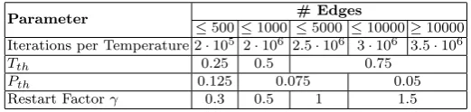
We provide results for 81 different graphs. We ran JAM a minimum of 5 times per instance, for the sake of statistical significance. We used different configurations that depended on the number of edges of the graph. In particular, the parameters being changed were the predefined number of iterations per temperature, Tth, Pth and γ. The values used can be found in Table 1. Other parameters used during the experiments which fixed for all the graph instances were the probability pN, fixed at a 0.9;λ, which was fixed to 0.1; andTs, which was fixed to 2· |V|.
Table 1.Parameters used depending on the number of edges of the graph
Parameter # Edges
≤500≤1000 ≤5000 ≤10000≥10000 Iterations per Temperature 2·105 2·106 2.5·106 3·106 3.5·106
Tth 0.25 0.5 0.75
Pth 0.125 0.075 0.05
Restart Factorγ 0.3 0.5 1 1.5
Numerical results There are three types of best known values (BKV) that can be found in Tables 2 and 3. The first ones are optimal results (in boldface); the second ones are values computed by heuristics and, hence, we do not know whether they are optimal or not. Finally we have instances for which only upper and lower bounds are found in the literature and are represented with a range of values. The BKVs from Table 2 come from works [28] and [30] and the upper/lower bounds from [5] and [6]. On the other hand, the BKVs from Table 3 come from [10, 7, 21, 33].
Table 2.Results for the minLA benchmark
Graph |V| |E| 1D 2D 3D
BKV δ Cost R C Cost R C Cost R C D Cost
bcspwr01 39 46 106 0% 106 3 13 57 5 8 51 2 4 5 50
bcspwr02 49 59 161 0% 161 7 7 72 - 2 5 5 66
bcspwr03 118 179 [588, 679] -2,50% 662 2 59 384 10 12 255 4 5 6 225
bcsstk01 48 176 1132 1,77% 1152 6 8 384 - 2 4 6 314
bcsstk02 66 2145 47916 -0,02% 47905 6 11 12155 8 9 11505 2 3 11 10945 bcsstk04 132 1758 [27569, 29804] 0,03% 29812 11 12 7126 - 3 4 11 5192 bcsstk05 153 1135 [9653, 11057] 0,02% 11059 9 17 11060 11 14 3508 2 7 11 2895
bcsstk22 110 254 - - 981 10 11 374 - 2 5 11 353
bintree10 1023 1022 3696 0% 3696 31 33 1231 32 32 1233 3 11 31 1098 c1y 828 1749 62230 0.33% 62436 23 36 5760 27 31 5752 6 6 23 3962 can 144 144 576 [2304, 3224] 0% 3224 12 12 1058 - 4 6 6 990 can 161 161 608 [5657, 6696] 0% 6696 7 23 1371 12 14 1253 4 6 7 1012
can 24 24 68 210 0% 210 4 6 98 - 2 3 4 98
can 61 61 248 1137 0% 1137 1 61 1137 7 9 485 3 3 7 425
can 62 62 78 [187, 212] -0,94% 210 2 31 130 7 9 90 3 3 7 84 can 73 73 152 [971, 1100] 0% 1100 1 73 1100 7 11 284 3 5 5 229 can 96 96 336 [2105, 2702] 0% 2702 8 12 600 9 11 599 4 4 6 525
curtis54 54 124 454 0% 454 6 9 194 7 8 191 3 3 6 179
dwt 162 162 510 [2032, 2431] 0,25% 2437 9 18 812 12 14 814 3 6 9 766 dwt 209 209 767 [5905, 6387] 20,78% 7714 11 19 1588 14 15 1653 5 6 7 1258 dwt 221 221 704 [3603, 3779] -0,13% 3774 13 17 1184 15 15 1176 5 5 9 1062 dwt 245 245 608 [3422, 3860] 4,53% 4035 7 35 1143 15 17 1054 5 7 7 920
dwt 59 59 104 289 0% 289 1 59 289 7 9 134 3 4 5 128
dwt 66 66 127 192 0% 192 6 11 164 8 9 163 2 3 11 159
dwt 72 72 75 167 0% 167 8 9 78 - 3 4 6 80
dwt 87 87 227 932 0% 932 3 29 448 8 11 384 2 4 11 334
fidap005 27 126 414 0% 414 5 6 250 - 3 3 3 242
fidapm05 1003 0% 1003 6 7 545 - 2 3 7 487
gd95c 62 144 506 0% 506 2 31 318 7 9 233 3 3 7 210
gd96b 111 193 1416 0% 1416 3 37 602 10 12 461 4 4 7 380
gd96c 65 125 519 0% 519 5 13 196 8 9 188 2 3 11 166
gd96d 180 228 2391 0% 2391 12 15 518 13 14 517 5 6 6 382
ibm32 32 90 485 0% 485 4 8 192 5 7 183 2 4 4 155
impcol b 59 281 [1810, 2076] 0% 2076 1 59 2076 7 9 713 3 4 5 588 lunda 147 1151 [10772, 11323] 0,03% 11326 7 21 2866 11 14 2802 3 7 7 2483 lundb 147 1147 [10712, 11187] 0,04% 11192 7 21 2836 11 14 2787 3 7 7 2452 mesh33x33 1089 2112 31729 3,03% 32693 33 33 2112 - 9 11 11 2764
nos4 100 247 1031 0% 1031 10 10 424 - 4 5 5 367
pores 1 30 103 383 0% 383 5 6 167 - 2 3 5 147
RandomA1 1000 4974 866968 3,00% 892986 25 40 57855 29 35 57436 10 10 10 26757 RandomA2 1000 24738 6522206 0,44% 6550805 25 40 427480 29 35 415460 10 10 10 196135
steam3 80 424 1416 0% 1416 8 10 946 - 4 4 5 842
tub100 100 148 246 0% 246 10 10 158 - 4 5 5 152
will57 57 127 335 0% 335 3 19 218 7 9 187 2 5 6 180
4 Conclusions
bench-Table 3.Results for the QAPlib benchmark
Graph |V| |E| 1D 2D 3D
Cost R C BKV δ Cost R C Cost R C D Cost
nug12 12 45 1000 3 4 578 0% 578 - 2 2 3 524
nug14 14 68 1866 3 5 1014 0% 1014 - 2 2 4 920
nug15 15 75 2186 3 5 1150 0% 1150 - 2 2 4 1030
nug16a 16 93 3050 4 5 1610 0% 1550 4 4 1550 2 2 4 1398 nug16b 16 84 2400 4 4 1240 0% 1240 4 4 1240 2 2 4 1130 nug17 17 101 3388 4 5 1732 0% 1672 3 6 1672 2 3 3 1466 nug18 18 113 3986 4 5 1930 0% 1900 3 6 1900 2 3 3 1646
nug20 20 141 5642 4 5 2570 0% 2570 - 2 2 5 2352
nug21 21 137 5084 3 7 2438 0% 2438 4 6 2270 2 3 4 1988 nug22 22 153 6184 2 11 3596 0% 3596 4 6 2742 2 3 4 2344
nug24 24 185 8270 4 6 3488 0% 3488 - 2 3 4 2938
nug25 25 200 9236 5 5 3744 0% 3744 - 3 3 3 3100
nug27 27 233 11768 3 9 5234 0% 5234 5 6 4612 3 3 3 3802 nug28 28 251 13090 4 7 5166 0% 5166 5 6 4988 2 3 5 4302
nug30 30 293 16502 5 6 6124 0% 6124 - 2 3 5 5240
scr12 12 28 42776 3 4 31410 0% 31410 - 2 2 3 30490 scr15 15 42 80862 4 4 51140 0% 51140 - 2 2 4 49968 scr20 20 62 183270 5 4 110030 0% 110030 - 2 2 5 101686 sko100a 100 3431 757188 10 10 152002 0,016% 152026 - 4 5 5 103176 sko100b 100 3414 771792 10 10 153890 0,005% 153898 - 4 5 5 104186 sko100c 100 3372 736510 10 10 147862 0% 147862 - 4 5 5 100438 sko100d 100 3367 747542 10 10 149576 0,011% 149592 - 4 5 5 101452 sko100e 100 3366 745104 10 10 149150 0,008% 149162 - 4 5 5 101330 sko100f 100 3377 746562 10 10 149036 0,005% 149044 - 4 5 5 100922 sko42 42 603 51050 6 7 15812 0% 15812 - 2 3 7 13758 sko49 49 811 81964 7 7 23386 0% 23386 - 2 5 5 18856 sko56 56 1061 128106 7 8 34458 0% 34458 - 2 4 7 28396 sko64 64 1386 193878 8 8 48498 0% 48498 - 4 4 4 34962 sko72 72 1781 278408 8 9 66256 0% 66256 - 3 4 6 48800 sko81 81 2274 410562 9 9 90998 0% 90998 - 3 3 9 73022 sko90 90 2771 547124 9 10 115534 0% 115534 - 3 5 6 82248 ste36a 34 172 20574 2 17 9526 0% 9526 5 7 9258 3 3 4 8226 tho150 150 4732 48711062 10 15 8133398 0,114% 8142732 12 13 7926106 5 5 6 5088332 tho30 30 217 348124 3 10149936 0% 149936 5 6 128772 2 3 5 109408 tho40 40 312 729452 4 10 240516 0% 240516 6 7 232752 2 4 5 192988 wil100 100 4459 1372700 10 10 273038 0% 273038 - 4 5 5 184756 wil50 50 1099 163508 5 10 48816 0% 48816 7 8 45672 2 5 5 37090
marks from the minLA and QAP literature. The results obtained with JAM often match the best known results and even improve some of them. Our experiments provide results for 1, 2 and 3 dimensions for 81 different graphs, broadening the available instances for both minLA and QAP as well as creating a valid set of benchmark instances for MAP.
References
1. Emile H.L. Aarts and P.J.M. van Laarhoven. Statistical cooling: A general ap-proach to combinatorial optimization problems. Philips Journal of Research, 40(4):193, 1985.
2. Una Benlic and Jin-Kao Hao. Breakout local search for the quadratic assignment problem. Applied Mathematics and Computation, 219(9):4800–4815, 2013. 3. Rainer E. Burkard, Stefan E. Karisch, and Franz Rendl. Qaplib–a quadratic
as-signment problem library. Journal of Global Optimization, 10(4):391–403, 1997. 4. R.E. Burkard and F. Rendl. A thermodynamically motivated simulation
proce-dure for combinatorial optimization problems. European Journal of Operational Research, 17(2):169 – 174, 1984.
5. Alberto Caprara, Adam N. Letchford, and Juan-Jos´e Salazar-Gonz´alez. Decorous lower bounds for minimum linear arrangement.INFORMS Journal on Computing, 23(1):26–40, 2011.
6. Alberto Caprara, Marcus Oswald, Gerhard Reinelt, Robert Schwarz, and Emiliano Traversi. Optimal linear arrangements using betweenness variables. Mathematical Programming Computation, 3(3):261–280, 2011.
7. David T. Connolly. An improved annealing scheme for the qap. European Journal of Operational Research, 46(1):93–100, 1990.
8. Zvi Drezner. Compounded genetic algorithms for the quadratic assignment prob-lem. Oper. Res. Lett., 33(5):475–480, 2005.
9. Matteo Fischetti, Michele Monaci, and Domenico Salvagnin. Three ideas for the quadratic assignment problem. Operations Research, 60(4):954–964, 2012. 10. Charles Fleurent and Jacques A. Ferland. Genetic hybrids for the quadratic
as-signment problem. InDIMACS Series in Mathematics and Theoretical Computer Science, pages 173–187. American Mathematical Society, 1993.
11. Charles Fleurent and Fred Glover. Improved constructive multistart strategies for the quadratic assignment problem using adaptive memory. INFORMS Journal on Computing, 11(2):198–204, 1999.
12. Mark D. Hansen. Approximation algorithms for geometric embeddings in the plane with applications to parallel processing problems. InFOCS, 1989., 30th Annual Symposium on, pages 604–609. IEEE, 1989.
13. Tabitha James, C´esar Rego, and Fred Glover. Multistart tabu search and di-versification strategies for the quadratic assignment problem. Systems, Man and Cybernetics, Part A: Systems and Humans, IEEE Trans. on, 39(3):579–596, 2009. 14. Zhu Jingwei, Rui Ting, Fang Husheng, Zhang Jinlin, and Liao Ming. Simulated
annealing ant colony algorithm for qap. InICNC 2012, pages 789–793, 2012. 15. Scott Kirkpatrick, D. Gelatt Jr., and Mario P Vecchi. Optimization by simmulated
annealing. Science, 220(4598):671–680, 1983.
16. Tjalling C. Koopmans and Martin Beckmann. Assignment problems and the lo-cation of economic activities. Econometrica: Journal of the Econometric Society, pages 53–76, 1957.
17. Yong Li, Panos M. Pardalos, and Mauricio G.C. Resende. A greedy randomized adaptive search procedure for the quadratic assignment problem. Quadratic As-signment and Related Problems, 16:237–261, 1994.
18. Andrew J. Mcallister. A new heuristic algorithm for the linear arrangement prob-lem. Technical Report TR-99-126a, University of New Brunswick, 1999.
20. Patrick Mills, Edward Tsang, and John Ford. Applying an extended guided local search to the quadratic assignment problem.Annals of Operations Research, 118(1-4):121–135, 2003.
21. Alfonsas Miseviˇcius. A modified simulated annealing algorithm for the quadratic assignment problem. Informatica, 14(4):497–514, 2003.
22. Alfonsas Miseviˇcius. An improved hybrid genetic algorithm: new results for the quadratic assignment problem. Knowl.-Based Syst., 17(2-4):65–73, 2004.
23. Alfonsas Miseviˇcius. A tabu search algorithm for the quadratic assignment prob-lem. Comp. Opt. and Appl., 30(1):95–111, 2005.
24. Alfonsas Miseviˇcius. An implementation of the iterated tabu search algorithm for the quadratic assignment problem. OR Spectrum, 34(3):665–690, 2012.
25. Volker Nissen and Henrik Paul. A modification of threshold accepting and its application to the quadratic assignment problem. Operations-Research-Spektrum, 17(2-3):205–210, 1995.
26. Axel Nyberg, Tapio Westerlund, and Andreas Lundell. Improved discrete refor-mulations for the quadratic assignment problem. In Integration of AI and OR Techniques in Constraint Programming for Combinatorial Optimization Problems, pages 193–203. Springer, 2013.
27. Jordi Petit. Experiments on the minimum linear arrangement problem. Journal of Experimental Algorithmics (JEA), 8:2–3, 2003.
28. Eduardo Rodr´ıguez-Tello, Jin-Kao Hao, and Jose Torres-Jim´enez. An effective two-stage simulated annealing algorithm for the minimum linear arrangement problem. Computers & Operations Research, 35(10):3331–3346, 2008.
29. Eduardo Rodr´ıguez-Tello and Jose Torres-Jim´enez. A refined evaluation function for the minla problem. InMICAI 2006, pages 392–403, 2006.
30. Ilya Safro, Dorit Ron, and Achi Brandt. Graph minimum linear arrangement by multilevel weighted edge contractions. Journal of Algorithms, 60(1):24–41, 2006. 31. Sartaj Sahni and Te´ofilo F. Gonz´alez. P-complete approximation problems. J.
ACM, 23(3):555–565, 1976.
32. Thomas St¨utzle. Max-min ant system for quadratic assignment problems. Tech-nical Report Forschungsbericht AIDA-97-04, TU Darmstadt, 1997.
33. ´Eric D. Taillard. Robust taboo search for the quadratic assignment problem. Parallel Computing, 17(4-5):443–455, 1991.
34. ´Eric D. Taillard and Luca Maria Gambardella. Adaptive memories for the quadratic assignment problems. Technical report, 1997.
35. James M. Varanelli and James P. Cohoon. A fast method for generalized starting temperature determination in homogeneous two-stage simulated annealing sys-tems. Computers & Operations Research, 26(5):481–503, 1999.
36. Jiunn-Chin Wang. Solving quadratic assignment problems by a tabu based simu-lated annealing algorithm. InICIAS 2007, pages 75–80. IEEE, 2007.
37. Jiunn-Chin Wang. A multistart simulated annealing algorithm for the quadratic assignment problem. InIBICA 2012, pages 19–23. IEEE, 2012.
38. Mickey R. Wilhelm and Thomas L. Ward. Solving quadratic assignment problems by simulated annealing. IIE Transactions, 19(1):107–119, 1987.