1
Causal Pathways for Temperature Predictability from Snow
Depth
†Erik W. Kolstad
Uni Research Climate, Bjerknes Centre for Climate Research, Jahnebakken 5, 5007 Bergen, Norway
Correspondence: [email protected]
† This version was accepted for publication in Journal of Climate on 22 August, 2017
Abstract: Dynamical subseasonal-to-seasonal (S2S) weather forecasting has made strides in recent years, thanks partly to better initialization and representation of physical variables in models. For instance, realistic initializations of snow and soil moisture in models yield enhanced temperature predictability on S2S time scales. Snow depth and soil moisture also mediate month-to-month persistence of near-surface air temperature. Here the role of snow depth as predictor of temperature one month ahead in the Northern Hemisphere is examined via two causal pathways. Through the first pathway, snow depth anomalies in month 1 persist into month 2 and are then linked to temperature anomalies through snow–temperature feedback mechanisms. The first pathway is active from fall to summer, and its effect peaks before the melting season: in winter in the low latitudes, in spring in the midlatitudes and in early summer in the high latitudes. The second pathway, where snow depth anomalies in month 1 lead to soil moisture anomalies in month 2 (through melting), which are then linked to temperature anomalies in month 2 through soil moisture–temperature feedbacks, is most active in spring and summer. The effect of the second pathway peaks during the melting season, namely later in the year than the first pathway. The latitudes of the highest mediated effect through both pathways follow a seasonal cycle, shifting northwards along with the seasonal insolation cycle. In keeping with this seasonal cycle, the highest snow depth mediation occurs to the north, and the highest soil moisture mediation to the south, of the latitudes with the highest overall temperature predictability from snow depth.
Keywords: snow depth; snow cover; soil moisture; snowmelt; seasonal prediction; land-atmosphere feedbacks
1. Introduction
Over the last few years, the skill of dynamical subseasonal-to-seasonal (S2S) forecast model systems has improved (Saha et al., 2013; Domeisen et al., 2014; Scaife et al., 2014; Dunstone et al., 2016; Weisheimer et al., 2017). The reasons include better representations of initial states, as well as improved parameterization of physical processes. For instance, realistic initialization of snow enhances the forecast skill of temperature on S2S time scales (Schlosser and Mocko, 2003; Peings et al., 2011; Jeong et al., 2012; Orsolini et al., 2013; Lin et al., 2016). Similar results have been obtained by initializing soil moisture (Dirmeyer, 2000; Douville, 2003; Conil et al., 2009; Koster et al., 2010; Koster et al., 2011; van den Hurk et al., 2012; Kumar et al., 2014), as well as both snow and soil moisture (Douville, 2010; Prodhomme et al., 2016; Thomas et al., 2016).
temperature was much reduced in snow-covered regions in the prescribed experiments. Both on regional scales and over large geographical distances, dynamical feedbacks between snow and the atmospheric circulation have also been identified (e.g., Foster et al., 1983; Cohen and Entekhabi, 1999; Yang et al., 2001; Cohen et al., 2007; Fletcher et al., 2009; Orsolini and Kvamstø, 2009; Sobolowski et al., 2010).
A number of physical feedback mechanisms exist between snow on the ground and the near-surface air temperature. The snow–albedo feedback (Thackeray and Fletcher, 2016) arises because snow has high albedo and reflects most of the incoming solar radiation, which leads to lower maximum air temperatures (Dewey, 1977). This impedes melting and therefore maintains the high surface albedo. A related feedback is associated with the low thermal conductivity of snow (Zhang, 2005). In winter, the air temperature can be considerable lower than the ground surface temperature, and then the deep snow prevents the air from being heated by from below. The feedback to the snow is that cold air inhibits melting. Furthermore, the high emissivity and large heat loss of snow leads to lower minimum temperatures (Dewey, 1977). Many empirical studies (Wagner, 1973; Walsh et al., 1982; Namias, 1985; Leathers and Robinson, 1993; Bednorz, 2004; Mote, 2008) and dynamical model experiments (e.g. Cohen and Rind, 1991; Yasunari et al., 1991; Vavrus, 2007; Alexander and Gong, 2011) have demonstrated the local cooling effect of snow.
Delayed effects of snow on air temperature have also been demonstrated. In spring, positive snow depth anomalies in one month can lead to positive soil moisture anomalies in subsequent months if the snow melts, as suggested by Walsh et al. (1985). According to Robock et al. (2000), soil moisture is, along with snow cover, ‘the most important component of meteorological memory for the climate system over the land’. Wet soils are conducive to cold temperature anomalies due to soil moisture–temperature feedback mechanisms (Dai et al., 1999; Fischer et al., 2007; Seneviratne et al., 2010). Conversely, negative snow depth anomalies can lead to future dry soil anomalies (due to lack of meltwater), which again can lead to warm temperature anomalies. These relationships between snow depth anomalies and subsequent soil moisture anomalies have been explored in numerous studies (e.g., Shinoda, 2001; Matsumura and Yamazaki, 2012; Potopová et al., 2016).
Here, the objective is to investigate the role of snow depth as an empirical predictor of near-surface air temperature (hereafter just ‘temperature’) anomalies one month ahead. This can be quantified with simple lagged correlations, but the focus here is on understanding how the predictability is carried forward from one month to the next. In other words, what are the physical mechanisms that act as mediators of the lagged influence of snow cover on temperature? Using methods from statistical mediation analysis (Baron and Kenny, 1986; MacKinnon et al., 2007), two causal pathways are investigated here to identify these mechanisms. A similar framework was recently used by Kolstad et al. (2017) to quantify the roles of snow depth, soil moisture and soil temperature in mediating month-to-month temperature persistence.
The physical mechanisms that form the components of the causal pathways—persistence of snow from one month to the next, the presence of snow and subsequent melting and soil moisture anomalies, and direct feedbacks between snow, soil moisture and temperature—are well-known. What is new here is that the roles of these mechanisms in mediating temperature predictability from month to month are quantified for each month of the year and for different latitudes. The results of the analysis are presented on large spatial scales and coarse temporal scales, but the methodology can be used as a template for more regionally detailed studies.
The paper is structured as follows. In Section 2, the theoretical foundation of the mediation analysis is described, and the data sources are introduced in Section 3. The results of the mediation analysis are presented in Section 4, and a summary and discussion of the results follow in Section 5.
2. Mediation analysis
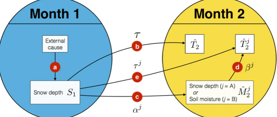
The indirect or mediated effects of the two causal pathways introduced earlier can be quantified using statistical mediation analysis. The predictor in month 1 is a snow depth anomaly, and is denoted as . The predictand in month 2 is a temperature anomaly, written as . The indirect effect of on is mediated by a mediator (snow depth or soil moisture) in month 2, denoted as , where the superscript j refers to the pathway. When j = A, the mediator is snow depth, and when j = B, soil moisture is the mediator. The pathways can be written as a causal chain (Pearl et al., 2016):
→ → . (1)
A causal chain illustrates a scenario where there is a direct effect of on , meaning that the two variables are significantly correlated. However, also has a direct effect on , and directly affects . If the causal chain describes full mediation (Baron and Kenny, 1986), becomes conditionally independent of given . This means that the entire effect of on is mediated by . If just some of the effect of on is mediated by , the causal chain describes partial mediation.
To formally check the validity of the mediation, three regressions, corresponding to Eqs. (1)-(3) in Fritz and MacKinnon (2007), are defined:
= + , (2)
= + + , (3)
= + , (4)
The carets on the left-hand sides symbolize that the values are estimated. in Eq. (2) is the predicted temperature in month 2, and the predictor in month 1 ( ). The total effect of on is the regression coefficient , and is the intercept. In Eq. (3), the mediator in month 2 ( ) is a regressor in addition to , and the predicted temperature has a superscript because it is predicted through Pathway j. The regression coefficients are and , and is the intercept. is also known as the effect of on adjusted for . In Eq. (4), is predicted by . The regression coefficient is the total effect of on , and is the intercept.
2) is shown with the arrow marked b, which leads from month 1 to the right oval, which represents month 2. To illustrate the first step of the mediation, the arrow marked c denotes the total effect of snow depth in month 1 on the mediator in month 2 ( in Eq. 4). The arrow marked d links and through the regression coefficient in Eq. (3), and the arrow marked esymbolizes the effect of on adjusted for ( in Eq. 4).
As mentioned, the causal framework allows both full and partial mediation. Four ‘steps’ must be satisfied for full mediation (Fritz and MacKinnon, 2007):
1. The total effect of on , i.e. in Eq. (2) and arrow b in Fig. 1, must be significant. 2. The total effect of on , i.e. in Eq. (4) and arrow c in Fig. 1, must be significant. 3. The effect of on controlled for , i.e. in Eq. (3) and arrow d in Fig. 1, must be significant.
4. The effect of on adjusted for , i.e. in Eq. (3) and arrow e in Fig. 1, must be non-significant.
A significance level of 5 percent was used throughout. For partial mediation, Step 4 is less strict and is only that < | |. This means that does not necessarily become conditionally independent of if is included in the regression, but the effect of on adjusted for is less than the total effect of on . Below, the criteria for partial mediation are used.
The definition of the mediated effect of on through Pathway j is the product ≝
. The mediated effects are calculated separately for the two mediators. If standardized anomalies are used, represents the partially mediated standardized temperature anomaly in month 2 for a +1 standard deviation snow depth anomaly in month 1 ( = 1), through mediation by snow depth or soil moisture anomalies in month 2. When = −1, the partially mediated standardized temperature anomaly in month 2 is − . Note that when partial mediation is considered, nonzero values of in Eq. (3) are allowed. This means that we cannot expect the (partially) mediated effect to be equal to the total effect .
3. Data
3.1. Data sources
The analysis is based on interannual time series of monthly mean 2-meter temperature, snow depth, and (volumetric) soil moisture in the surface layer (0–10 cm). To account for enhanced interannual autocorrelations due to long-term trends, each time series was detrended by subtracting the best linear least squares fit (with negligible impact on the results).
The two main data sources are the NOAA-CIRES Twentieth Century Reanalysis (Compo et al., 2011), version 2c (20CR henceforth), and the ECMWF’s ERA-20C reanalysis (Poli et al., 2016). The 20CR covers the period 1850–2014, but only the period 1900–2010 was used, because it overlaps with the ERA-20C period. The 20CR assimilates sea surface temperatures, sea ice and surface pressure, while the ERA-20C ingests surface winds as well. This means that their temperature, snow, and soil moisture fields are model-derived and may differ from observations. The representation of snow varies across reanalysis products. Comparing eight modern-era reanalyses, Mudryk et al. (2015) concluded that the spread in snow mass climatology were due to differences in the land surface models, but that the day-to-day correlations of snow anomalies were controlled by the atmospheric forcing. Such findings have inspired to production of offline land-surface models, forced by atmospheric fields from other reanalyses. One of these is ERA-Interim/Land reanalysis (Balsamo et al., 2015), an offline land-surface model run with atmospheric forcing from ERA-Interim (Dee et al., 2011), with precipitation adjustments based on observations. ERA-Interim/Land is used here as a reference data set. Another offline product is MERRA-Land (Reichle et al., 2011), which was forced with atmospheric fields from MERRA (Rienecker et al., 2011). But as the main improvements of MERRA-Land relative to MERRA were carried into the higher-resolution MERRA-2 (Gelaro et al., 2017), and “MERRA-2 land hydrology estimates are better than those of MERRA-Land” (Reichle et al., 2017), MERRA-2 is used here rather than MERRA-Land. Both ERA-Interim and MERRA-2 are satellite-era reanalyses and assimilate a multitude of observations and remotely sensed data.
How do the two twentieth century reanalyses perform? Zampieri et al. (2016) found that 20CR and ERA-20C reproduced a heat wave index reasonably well compared to satellite-era reanalyses. The variability of daily soil moisture in 20CR was contrasted with other reanalyses and observational networks by Dirmeyer et al. (2016), and was found to have a consistent negative bias. ERA-Interim/Land had an average positive bias of similar magnitude. ERA-20C was not evaluated. As for snow, the onset of autumnal snowfall in Eurasia in 20CR was found by Peings et al. (2013) to correspond well with observations. The snow depth in both reanalyses was evaluated by Wegmann et al. (2016), using in-situ observations from Russian stations as reference. They found that ERA-20C had lower snow depths than 20CR at the start of the 20th century,
yielding a positive trend over the century in ERA-20C. No such trend was found in 20CR. In the satellite era, the geographical pattern of snow depths was found to correspond reasonably well with observations, except that 20CR was overestimated the snow depth somewhat, while ERA-20C had lower snow depths in Northern Siberia.
3.2. Comparison of the reanalyses
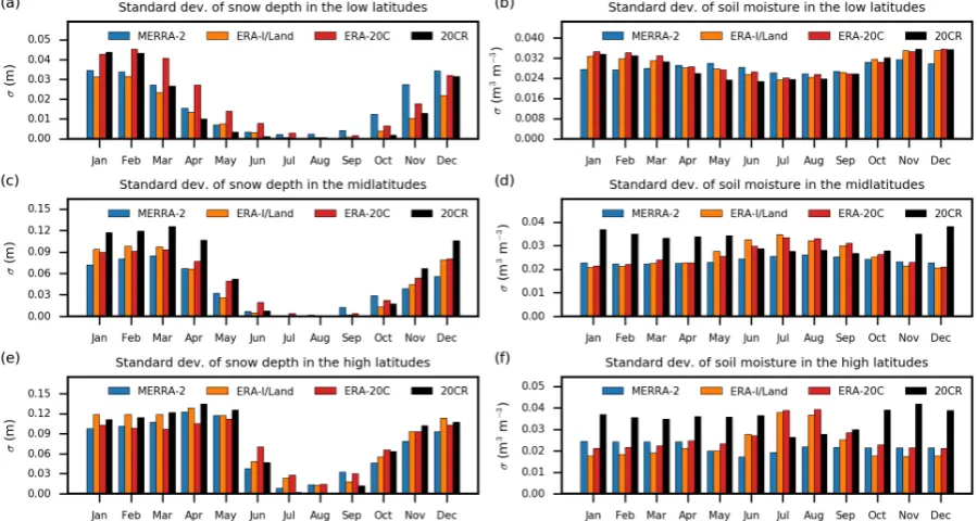
mean, as standardized anomalies are used in Eqs. (2–4). Noting the narrow ranges of the y-axes for the low latitudes in Fig. 2a, the differences between the reanalyses are practically negligible. In the midlatitudes (Fig. 2b), the most notable difference is that 20CR has the strongest variability in winter and spring. The average standard deviation in the high latitudes (Fig. 2c) is comparable across the reanalyses except for the high values in ERA-Interim/Land in December. The area-averaged standard deviation of soil moisture in the low latitudes is comparable in all the data sets (Fig. 2d). In the midlatitudes, the interannual variability (Fig. 2e) is substantially higher in 20CR than in the other products from fall to spring. In summer, the variability is somewhat higher in ERA-Interim/Land and ERA-20C. This pattern is repeated in the high latitudes (Fig. 2f), with even larger differences between the variability in ERA-Interim/Land and ERA-20C compared to MERRA-2 and 20CR in summer. In summary, it is difficult to judge whether any of the data sets is ‘better’ than the others. The strategy used in the remaining analysis is to use both 20CR and ERA-20C, as these reanalyses, while both are imperfect, provide the longest time series (1900– 2010) and therefore yield more statistical robustness than the modern-era reanalyses (1980 to present). To assess the validity of the results, the first and second halves of the period 1900–2010 are also analyzed separately.
Fig. 2. Standard deviation of snow depth in meters (a, c, and e) and dimensionless volumetric soil moisture (b, d, and f) during the period 1980–2010, according to ERA-Interim/Land, MERRA-2, ERA-20C, and 20CR, as indicated. The values are area-averaged in three latitude belts: (a–b) the low latitudes (30N–45N), (c–d) the midlatitudes (45N–60N), and (e–f) the high latitudes (60N–75N).
3.3. Some technical notes
means of 6-hourly calculated snow depth with monthly mean SWE divided by monthly mean snow density in ERA-Interim/Land gave practically identical results. Another technical note is that in all the data sets, grid points for which the long-term mean August snow depth exceeds 1 meter are excluded from the analysis. This was done to focus on locations with seasonal snow cover and to mask out glaciers. In addition, when analyzing interannual time series for specific months, grid points for which the interannual maximum snow depth was less than 10 cm were also excluded (to mask out locations where snow fluctuations are unimportant).
4. Results
4.1. Temperature predictability and its pathways in March/April
In this section, the focus is on one particular month pair to illustrate the geographical distributions of the total and mediated effects of snow depth on temperature. Later in the text, zonal means and area-averaged values of the total effect (which is independent of the pathways) and the mediated effects through pathways A and B (i.e., and ) are analyzed for different parts of the year.
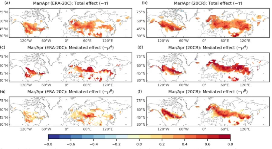
Figs. 3a–b show the total lagged effect for each land grid point (except for the masked grid points and where the correlation is non-significant) north of 27N for March/April. Note that the variable shown is – because is negative everywhere. The reanalyses agree quite well on the geographical patterns. Both have local maxima of − north in Eastern Europe, in Kazakhstan, around the Tibetan Plateau, and in a belt in North America stretching from New England to Alberta. Broadly speaking, high − values occur in the humid continental climate zones of both continents. The mediated effect through Pathway A is shown as − in Figs. 3c–d wherever the pathway is valid. Note that is significant in many locations where Pathway A is not valid, such as in parts of the Rocky Mountains and Eastern Europe. This means that snow depth in month 1 has an effect on temperature in month 2, but this effect is not mediated through Pathway A. The highest − values tend to occur slightly north of the highest − values, while the highest mediated effect through Pathway B (shown as − in Figs. 3e–f) occurs slightly south of the highest − values. A zonal mean analysis below shows that this is a generally valid feature from late winter to early summer.
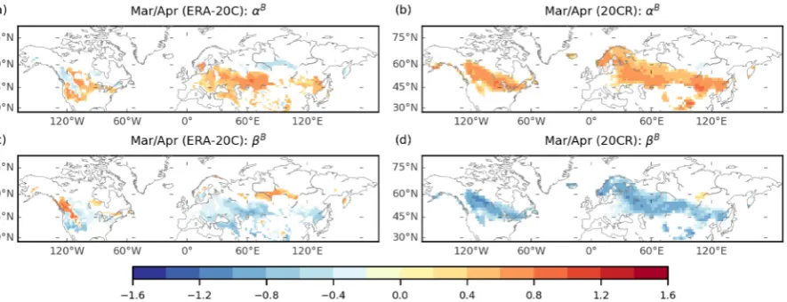
For Pathway B, for which and are shown in Fig. 5, we note first that and generally have opposite signs ( < 0). In contrast to , which is positive nearly everywhere,
(the lag-1 correlation coefficient between snow depth in March and soil moisture in April) has both positive and negative values (Figs. 5a–b). The physical mechanisms that lead to negative values vary with the sign of . Where > 0 and < 0, positive snow depth anomalies in March ( > 0) are associated with positive soil moisture anomalies and cold temperature anomalies in April. Negative snow depth anomalies in March ( < 0) yield negative soil moisture anomalies and warm temperature anomalies in April. In the regions where < 0 and > 0, positive snow depth anomalies in March ( > 0) are linked to negative soil moisture anomalies and negative temperature anomalies in April, and negative snow depth anomalies in March ( < 0) lead to positive anomalies in both soil moisture and temperature in April. There are some geographical differences between the reanalyses. In some northern and high-altitude locations in ERA-20C, is negative (Fig. 5a) and is positive (Fig. 5c). In 20CR, is mainly positive (Fig. 5b) and negative (Fig. 5c), and the northernmost extent of positive values is located farther farther north than in ERA-20C.
The geographical distributions of , , and are only shown for the March/April month pair, but these months were chosen because they are representative for the period from late winter to early summer. As will be shown below, these are the times of the year when Pathway B is most active. In fall and early winter, the mediation is carried out through Pathway A. In late summer, there is little seasonal snow cover even in the high latitudes and hence little predictability from snow.
Fig. 4. (a–b) Maps of and (c–d) for March/April in the period 1900–2010 wherever Pathway Pathway A is valid. The colors in all the panels correspond to the legend at the bottom. The unit is standard deviations.
Fig. 5. (a–b) Maps of and (c–d) for March/April in the period 1900–2010 wherever Pathway Pathway B is valid. The colors in all the panels correspond to the legend at the bottom. The unit is standard deviations.
4.2. Zonally averaged total and mediated effects
Following up on the apparent result that the highest values of occur to the north (and to the south) of the highest values, zonal means of the direct and mediated effects are now calculated. A moving average spanning five latitude degrees is applied to smooth the sometimes noisy ‘raw’ zonal mean values. Figure 6 shows − ̅, − , and − for the two data sets in March/April. The minus signs are added because the zonal mean values are mainly negative, and the overbars symbolize the zonal averaging. The latitudes of the maximum values of the zonal means − ̅, − , and − are defined as , , and , respectively. The blue solid curve shows shows that is 50N, and that both and are 48N in ERA-20C. In 20CR , , and are 50N, 52N, and 54N, respectively.
Table 1 for month pairs from winter to summer for both reanalyses. The following inequalities are always satisfied for these months: ≥ ≥ . This means that for zonal means, mediation by soil moisture is systematically most active at or to the south, and snow depth mediation at or to the north, of the latitudes with the highest temperature predictability from snow depth.
Fig. 6. Zonal means of − (orange), − (blue) and − (red) for ERA-20C (solid curves) and 20CR (dashed curves) for March/April in the period 1900–2010. The unit is standard deviations.
Table 1. Latitudes of maximum zonal mean values of − , − , and − , all in degrees north.
Data set ERA-20C 20CR
Month pair
Jan/Feb 35 36 36 39 39 41
Feb/Mar 44 47 47 45 47 47
Mar/Apr 48 48 50 49 50 54
Apr/May 58 61 62 56 56 60
May/Jun 64 66 68 66 66 70
Jun/Jul 71 71 74 71 71 73
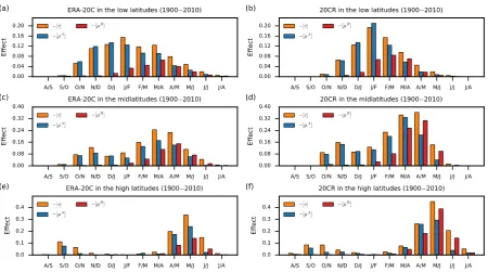
4.3. Area-averaged total and mediated effects
Figure 7 show −[ ], where the brackets indicate area-averaging and the minus sign is used because all the [ ] values are negative. When calculating the area-averaged values, grid points for which is not significant at the 5 percent level are given zero weight, but the areas of the grid points still count towards the total areas used for averaging. The relative roles of the two pathways can be assessed through the area-averaged values of the mediated effects, i.e. −[ ] and −[ ], shown in Fig. 7 as blue and red bars, respectively. For these metrics, the values in grid points where the respective pathway is invalid are given zero weight. Although not shown here, the equivalents of Fig. 7 for the two halves of the 1900–2010 period, i.e. 1900–1955 and 1956–2010, have been calculated separately, with the time series of all the variables detrended over the individual periods. The results for those two periods are sufficiently similar to each other and to the one in Fig. 7 that it can be concluded that the results are robust with respect to time period.
In the low latitudes (Figs. 7a–b), −[ ] follows a seasonal cycle with non-zero values first appearing in October/November, a peak in January/February, and then gradually declining values towards summer. There is good agreement between the reanalyses on the seasonal cycle. The nonzero values in fall and summer mainly stem from isolated high-altitude locations. The blue bars show that −[ ] has nonzero values from fall to spring. In winter, −[ ] closely agrees with
−[ ], but after winter the ratio [ ]/[ ] gradually decreases. The red bars show that −[ ] has a more contracted seasonal cycle than −[ ]. Nonzero −[ ] values occur from early winter to early summer. The peak of −[ ] in spring occurs three months after the peak of −[ ] in ERA-20C and one month after in ERA-20CR.
In the midlatitudes, the values of all the three metrics are generally higher in 20CR (Fig. 7d) than in ERA-20C (Fig. 7c). As in the low latitudes, the seasonal cycle of nonzero −[ ] values starts in fall and ends in summer, but the peak occurs in spring, not in winter. The values of −[ ]
around the peak are also higher than in the low latitudes. The values of −[ ] peak in March/April in both data sets, and after this the ratio [ ]/[ ] gradually decreases, as in the low latitudes. The seasonal cycle of −[ ] starts about one month later than in the low latitudes, and the timing of the peak is also shifted closer to summer (one month in ERA-20C and two months in 20CR).
Fig. 7. In each panel, area-averaged values of − (orange bars), − (blue bars) and − (red bars) in 1900–2010 are shown for the whole year for three latitude belts: (a–b) the low latitudes (30N–45N), (c–d) the midlatitudes (45N–60N), and (e–f) the high latitudes (60N–75N). The left column (a, c, and e) shows results for ERA-20C, and the right column (b, d, and f) for 20CR. The unit is standard deviations.
5. Discussion
It is already well-known from previous studies that snow anomalies impart temperature predictability on S2S time scales. What is new in this study is that physical mechanisms for this predictability have been quantified systematically in the extratropical Northern Hemisphere. Two causal pathways have been investigated, one based on month-to-month persistence of snow depth anomalies and another that describes the delayed effect of snow depth anomalies mediated by soil moisture anomalies in the subsequent month.
in April—provided that the lag-1 autocorrelation of snow depth is positive. Note also that the specification anomalous is sometimes omitted for readability.)
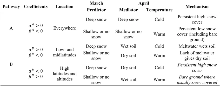
Table 2. A summary of the proposed physical mechanisms for temperature predictability from snow depth for both pathways in March/April. The first two rows describe Pathway A and the last four rows Pathway B. The last two proposed mechanisms are in italics because they are open to question.
Pathway Coefficients Location March April Mechanism
Predictor Mediator Temperature
A > 0< 0 Everywhere
Deep snow Deep snow Cold Persistent high snow cover
Shallow or no snow
Shallow or no
snow Warm
Persistent low snow cover (including bare
ground)
B
> 0
< 0 midlatitudes Low- and
Deep snow Wet soil Cold Meltwater wets soil
Shallow or no
snow Dry soil Warm
Lack of meltwater gives dry soil
< 0 > 0
High latitudes and
altitudes
Deep snow Dry soil Cold Persistent high snow
cover
Shallow or no
snow Wet soil Warm
Bare ground where usually snow covered
Pathway A describes persistence of snow depth anomalies from one month to the next. This is clear from the maps in Figs. 4a–b, which show that is positive where Pathway A is valid. As indicated in the first row of Table 2, this implies that when there is anomalously deep snow in March, the snow in April will also be anomalously deep. Such conditions are associated with anomalous cooling of the air near the surface through the physical mechanisms described in the Introduction (albedo feedback, insulation, and high emissivity and heat loss). The cooling of the air is part of a positive feedback mechanism, as the cooling will impede melting and thereby help to preserve the above-normal snow depth. The second row in Table 2 states that when there is anomalously little snow in March, either because there is just a shallow snow layer or there is no snow, the snow depth will continue to be anomalously low in April (as > 0). Unusually shallow shallow (or absent) snow is associated with warmer-than-normal air temperatures, due to the absence of cooling mechanisms. The warming of the air from below is also part of a positive feedback mechanism, as the anomalously warm air promotes further reductions of the snow depth through melting.
< 0, the dry soil in April is associated with to anomalously warm temperatures, also due to soil moisture–temperature feedbacks. It seems reasonable to infer that the regions where > 0 and
< 0 consist of locations where snow usually melts from March to April. When there is more snow than usual in March, the soil becomes wetter-than-normal in April, and this leads to warm temperature anomalies through well-known soil moisture–temperature feedbacks (Seneviratne et al., 2010). The same feedbacks come into play when there is less snow than normal in March. This gives a deficit of meltwater and hence the soil becomes drier-than-normal in April, leading to warm temperature anomalies through the same feedback mechanisms.
When > 0 and < 0, the mechanisms outlined above and in the first four rows of Table 2 are straightforward. Figure 5 shows that negative values are also possible. In some regions, < 0 and > 0 in March/April. The mediated effect is still negative, but when anomalously deep snow in March is the predictor, anomalously dry soil and cold temperature anomalies follow in April. And conversely, an anomalously shallow snow cover in March is followed by anomalously wet soil and warm temperatures in April. Both temperature outcomes are contrary to what would be expected from soil moisture–temperature feedbacks. The mechanisms for the cases where < 0 and > 0 are therefore not obvious.
As shown in Fig. 5, < 0 and > 0 mainly in ERA-20 and only in the high altitudes (e.g. in the Rocky Mountains) and in subarctic climate zones (Peel et al., 2007), where the climatological temperatures are probably colder than where > 0 and < 0. Although not shown, in support of this notion the few regions where < 0 and > 0 are found even farther north in April/May than in March/April. It is therefore likely that the regions where < 0 and
> 0 form the boundary between regions where snow usually melts from March to April (i.e. where > 0 and < 0; see Fig. 5) and the regions where snow practically never melts between between those two months (i.e. in even higher latitudes or altitudes, where Pathway B is not valid; see white areas in Fig. 5). This suggests that the following mechanisms take place, although it must be emphasized that the proposed mechanisms are open to quesion.
Let us first consider the case when the snow depth is unusually high in March. This could occur because the previous fall was colder-than-normal, with unusually early snow onset and anomalously dry soils due to below-normal rainfall. The soils will stay anomalously dry due to persistence beneath the snow cover. Since the climatological temperatures in March/April are cold, the deeper-than-usual snow cover in March is unlikely to melt by April. If the snow is still present in April, the temperature is anomalously low due to the same snow–temperature feedback mechanisms described earlier. The second case is that there is unusually shallow snow in March. This makes it more likely that the snow cover melts by April. If the snow does melt, the soil will become anomalously wet. (The below-normal snow depth in March could also be due to later-than-normal snow onset during the previous fall, and then the soil would already be wetter-than-normal beneath the snow throughout winter.) The ground is then bare, and the lack of cooling snow–temperature feedbacks yields higher-than-normal temperatures.
If the proposed mechanisms where < 0 and > 0 outlined here are correct, the soil moisture anomalies in April are not the real causes of the anomalous temperatures in April, although Pathway B satisfies all the four steps required for mediation in both cases. These cases are useful reminders that statistical causality analysis must always be paired with physical considerations. The two proposed mechanisms are listed in the last two rows of Table 2 (in italics because they are somewhat speculative).
found. The latitudes of the highest zonal mean values in Table increase steadily with each month for all the variables. This suggests that the annual cycles of predictability and mediation through both pathways are driven by the annual cycle of insolation, and by implication, the annual cycle of melting.
Area-averaged values of the total effect of snow depth on temperature ([ ]) and the mediated effect through Pathways A ([ ]) and B ([ ]) were investigated in Section 4c (see Fig. 7). As in March/April, [ ] is either zero or negative. This means that, on average, positive snow depth anomalies in month 1 are associated with negative temperature anomalies in month 2. This occurs from fall to summer in the low- and midlatitudes, and in fall and from spring to summer in the high latitudes. In all the latitude belts, the annual cycle of the mediated effect through Pathway A starts earlier and peaks earlier than the mediated effect through Pathway B. In other words, persistence of snow depth anomalies from one month to the next is the main mediator of temperature persistence early in the seasonal cycle of the persistence. Towards the end of the season, when the seasonal snow cover starts to melt, the relative role of the delayed effect of snow depth anomalies on soil moisture anomalies becomes greater.
The analysis presented here is aggregated for large regions. Local variations and particularities are omitted. For example, melting snow in one location (e.g. from glaciers) could add moisture to the soil in neighboring locations through transportation in rivers. Such interactions on local scales are not studied here, where a grid point by grid point approach has been used. However, the methodology illustrates how simple linear regressions can be powerful tools when applied in the framework of statistical mediation analysis. It is hoped that, together with other climate-related studies that have made use of causality analysis (e.g. Ebert-Uphoff and Deng, 2012; Runge et al., 2013; Kretschmer et al., 2016; Kretschmer et al., 2017), this provides stimulus for future studies of complex, multivariate and regional climatic interactions.
Acknowledgments
The author wishes to thank three anonymous referees for reviews that led to an improved paper, and Stefan Sobolowski and Yvan Orsolini for useful comments on an earlier version of the text. Funding was given by the Research Council of Norway through the SNOWGLACE (grant 244166) and Seasonal Forecast Engine (grant 270733) projects. The 20CR data was downloaded from doi:10.5065/D6N877TW, and MERRA-2 from doi: 10.5067/8S35XF81C28F. The European Centre for Medium-Range Weather Forecasts (ECMWF) provided the 20C and ERA-Interim/Land reanalyses, and the Global Modeling and Assimilation Office (GMAO) at NASA Goddard Space Flight Center provided the MERRA-2 data. Support for the Twentieth Century Reanalysis Project dataset is provided by the U.S. Department of Energy, Office of Science Innovative and Novel Computational Impact on Theory and Experiment (DOE INCITE) program, and Office of Biological and Environmental Research (BER), and by the National Oceanic and Atmospheric Administration (NOAA) Climate Program Office.
References
1. Alexander, P. and G. Gong, 2011: Modeled surface air temperature response to snow depth variability. J. Geophys. Res. Atmos., 116, D14105, doi:10.1029/2010JD014908.
3. Baron, R. M. and D. A. Kenny, 1986: The moderator–mediator variable distinction in social psychological research: Conceptual, strategic, and statistical considerations. Journal of Personality and Social Psychology, 51, 1173–1182, doi:10.1037/0022-3514.51.6.1173.
4. Bednorz, E., 2004: Snow cover in eastern Europe in relation to temperature, precipitation and circulation. Int. J. Climatol., 24, 591-601, doi:10.1002/joc.1014.
5. Cohen, J. and D. Rind, 1991: The Effect of Snow Cover on the Climate. J. Clim., 4, 689-706, doi:10.1175/1520-0442(1991)004<0689:TEOSCO>2.0.CO;2.
6. Cohen, J. and D. Entekhabi, 1999: Eurasian snow cover variability and Northern Hemisphere climate predictability. Geophys. Res. Lett., 26, 345-348, doi:10.1029/1998gl900321.
7. Cohen, J., M. Barlow, P. J. Kushner, and K. Saito, 2007: Stratosphere–Troposphere Coupling and
Links with Eurasian Land Surface Variability. J. Clim., 20, 5335–5343,
doi:10.1175/2007JCLI1725.1.
8. Compo, G. P., and Coauthors, 2011: The Twentieth Century Reanalysis Project. Q. J. R. Meteorol. Soc., 137, 1-28, doi:10.1002/qj.776.
9. Conil, S., H. Douville, and S. Tyteca, 2009: Contribution of realistic soil moisture initial conditions to boreal summer climate predictability. Clim. Dyn., 32, 75–93, doi:10.1007/s00382-008-0375-9. 10. Dai, A., K. E. Trenberth, and T. R. Karl, 1999: Effects of Clouds, Soil Moisture, Precipitation, and
Water Vapor on Diurnal Temperature Range. J. Clim., 12, 2451–2473, doi:10.1175/1520-0442(1999)012<2451:EOCSMP>2.0.CO;2.
11. Dee, D. P., and Coauthors, 2011: The ERA-Interim reanalysis: Configuration and performance of the data assimilation system. Q. J. R. Meteorol. Soc., 137, 553-597, doi:10.1002/qj.828.
12. Dewey, K. F., 1977: Daily Maximum and Minimum Temperature Forecasts and the Influence of
Snow Cover. Mon. Weather Rev., 105, 1594-1597,
doi:10.1175/1520-0493(1977)105<1594:DMAMTF>2.0.CO;2.
13. Dirmeyer, P. A., 2000: Using a Global Soil Wetness Dataset to Improve Seasonal Climate
Simulation. J. Clim., 13, 2900-2922,
doi:10.1175/1520-0442(2000)013<2900:UAGSWD>2.0.CO;2.
14. Dirmeyer, P. A., and Coauthors, 2016: Confronting Weather and Climate Models with Observational Data from Soil Moisture Networks over the United States. Journal of Hydrometeorology, 17, 1049-1067, doi:10.1175/JHM-D-15-0196.1.
15. Domeisen, D. I. V., A. H. Butler, K. Fröhlich, M. Bittner, W. A. Müller, and J. Baehr, 2014: Seasonal Predictability over Europe Arising from El Niño and Stratospheric Variability in the MPI-ESM Seasonal Prediction System. J. Clim., 28, 256-271, doi:10.1175/JCLI-D-14-00207.1. 16. Douville, H., 2003: Assessing the influence of soil moisture on seasonal climate variability with
AGCMs. Journal of Hydrometeorology, 4, 1044–1066,
doi:10.1175/1525-7541(2003)004<1044:ATIOSM>2.0.CO;2.
17. Douville, H., 2010: Relative contribution of soil moisture and snow mass to seasonal climate predictability: a pilot study. Clim. Dyn., 34, 797–818, doi:10.1007/s00382-008-0508-1.
18. Dunstone, N., D. Smith, A. Scaife, L. Hermanson, R. Eade, N. Robinson, M. Andrews, and J. Knight, 2016: Skilful predictions of the winter North Atlantic Oscillation one year ahead. Nat. Geosci., 9, 809–814, doi:10.1038/ngeo2824.
19. Dutra, E., C. Schär, P. Viterbo, and P. M. A. Miranda, 2011: Land-atmosphere coupling associated with snow cover. Geophys. Res. Lett., 38, L15707, doi:10.1029/2011GL048435.
20. Ebert-Uphoff, I. and Y. Deng, 2012: Causal Discovery for Climate Research Using Graphical Models. J. Clim., 25, 5648-5665, doi:10.1175/JCLI-D-11-00387.1.
21. Fischer, E. M., S. I. Seneviratne, D. Lüthi, and C. Schär, 2007: Contribution of land-atmosphere coupling to recent European summer heat waves. Geophys. Res. Lett., 34, L06707, doi:10.1029/2006GL029068.
23. Foster, J., M. Owe, and A. Rango, 1983: Snow Cover and Temperature Relationships in North America and Eurasia. Journal of Climate and Applied Meteorology, 22, 460-469, doi:10.1175/1520-0450(1983)022<0460:SCATRI>2.0.CO;2.
24. Fritz, M. S. and D. P. MacKinnon, 2007: Required Sample Size to Detect the Mediated Effect. Psychological science, 18, 233-239, doi:10.1111/j.1467-9280.2007.01882.x.
25. Gelaro, R., and Coauthors, 2017: The Modern-Era Retrospective Analysis for Research and Applications, Version 2 (MERRA-2). J. Clim., 30, 5419–5454, doi:10.1175/JCLI-D-16-0758.1. 26. Jeong, J.-H., H. W. Linderholm, S.-H. Woo, C. Folland, B.-M. Kim, S.-J. Kim, and D. Chen, 2012:
Impacts of Snow Initialization on Subseasonal Forecasts of Surface Air Temperature for the Cold Season. J. Clim., 26, 1956-1972, doi:10.1175/JCLI-D-12-00159.1.
27. Kolstad, E. W., E. A. Barnes, and S. P. Sobolowski, 2017: Quantifying the Role of Land– Atmosphere Feedbacks in Mediating Near-Surface Temperature Persistence. Q. J. R. Meteorol. Soc., 143, 1620–1631, doi:10.1002/qj.3033.
28. Koster, R. D., and Coauthors, 2011: The Second Phase of the Global Land–Atmosphere Coupling Experiment: Soil Moisture Contributions to Subseasonal Forecast Skill. Journal of Hydrometeorology, 12, 805-822, doi:10.1175/2011JHM1365.1.
29. Koster, R. D., and Coauthors, 2010: Contribution of land surface initialization to subseasonal forecast skill: First results from a multi-model experiment. Geophys. Res. Lett., 37, L02402, doi:10.1029/2009GL041677.
30. Kretschmer, M., J. Runge, and D. Coumou, 2017: Early prediction of extreme stratospheric polar vortex states based on causal precursors. Geophys. Res. Lett., in press, doi:10.1002/2017GL074696.
31. Kretschmer, M., D. Coumou, J. F. Donges, and J. Runge, 2016: Using Causal Effect Networks to Analyze Different Arctic Drivers of Midlatitude Winter Circulation. J. Clim., 29, 4069-4081, doi:10.1175/JCLI-D-15-0654.1.
32. Kumar, S., and Coauthors, 2014: Effects of realistic land surface initializations on subseasonal to seasonal soil moisture and temperature predictability in North America and in changing climate simulated by CCSM4. J. Geophys. Res. Atmos., 119, 13,250-13,270, doi:10.1002/2014JD022110. 33. Leathers, D. J. and D. A. Robinson, 1993: The Association between Extremes in North American
Snow Cover Extent and United States Temperatures. J. Clim., 6, 1345-1355, doi:10.1175/1520-0442(1993)006<1345:TABEIN>2.0.CO;2.
34. Lin, P., J. Wei, Z.-L. Yang, Y. Zhang, and K. Zhang, 2016: Snow data assimilation-constrained land initialization improves seasonal temperature prediction. Geophys. Res. Lett., 43, 11,423-11,432, doi:10.1002/2016GL070966.
35. MacKinnon, D. P., A. J. Fairchild, and M. S. Fritz, 2007: Mediation analysis. Annu. Rev. Psychol., 58, 593–614, doi:10.1146/annurev.psych.58.110405.085542.
36. Matsumura, S. and K. Yamazaki, 2012: A longer climate memory carried by soil freeze–thaw processes in Siberia. Environ. Res. Lett., 7, 045402, doi:10.1088/1748-9326/7/4/045402.
37. Mote, T. L., 2008: On the Role of Snow Cover in Depressing Air Temperature. Journal of Applied Meteorology and Climatology, 47, 2008-2022, doi:10.1175/2007JAMC1823.1.
38. Mudryk, L. R., C. Derksen, P. J. Kushner, and R. Brown, 2015: Characterization of Northern Hemisphere Snow Water Equivalent Datasets, 1981–2010. J. Clim., 28, 8037–8051, doi:10.1175/JCLI-D-15-0229.1.
39. Namias, J., 1985: Some empirical evidence for the influence of snow cover on temperature and
precipitation. Mon. Weather Rev., 113, 1542–1553,
doi:10.1175/1520-0493(1985)113<1542:SEEFTI>2.0.CO;2.
41. Orsolini, Y. J. and N. G. Kvamstø, 2009: Role of Eurasian snow cover in wintertime circulation: Decadal simulations forced with satellite observations. J. Geophys. Res., 114, D19108, doi:10.1029/2009jd012253.
42. Pearl, J., M. Glymour, and N. P. Jewell, 2016: Causal Inference in Statistics: A Primer. Wiley. 43. Peel, M., B. Finlayson, and T. McMahon, 2007: Updated world map of the Koppen-Geiger climate
classification. Hydrol. Earth Syst. Sci., 11, 1633–1644, doi:10.5194/hess-11-1633-2007.
44. Peings, Y., H. Douville, R. Alkama, and B. Decharme, 2011: Snow contribution to springtime atmospheric predictability over the second half of the twentieth century. Clim. Dyn., 37, 985–1004, doi:10.1007/s00382-010-0884-1.
45. Peings, Y., E. Brun, V. Mauvais, and H. Douville, 2013: How stationary is the relationship between Siberian snow and Arctic Oscillation over the 20th century? Geophys. Res. Lett., 40, 183-188, doi:10.1029/2012GL054083.
46. Poli, P., and Coauthors, 2016: ERA-20C: An Atmospheric Reanalysis of the Twentieth Century. J. Clim., 29, 4083-4097, doi:10.1175/JCLI-D-15-0556.1.
47. Potopová, V., C. Boroneanţ, M. Možný, and J. Soukup, 2016: Driving role of snow cover on soil moisture and drought development during the growing season in the Czech Republic. Int. J. Climatol., 36, 3741-3758, doi:10.1002/joc.4588.
48. Prodhomme, C., F. Doblas-Reyes, O. Bellprat, and E. Dutra, 2016: Impact of land-surface initialization on sub-seasonal to seasonal forecasts over Europe. Clim. Dyn., 47, 919-935, doi:10.1007/s00382-015-2879-4.
49. Reichle, R. H., R. D. Koster, G. J. M. De Lannoy, B. A. Forman, Q. Liu, S. P. P. Mahanama, and A. Touré, 2011: Assessment and Enhancement of MERRA Land Surface Hydrology Estimates. J. Clim., 24, 6322-6338, doi:10.1175/JCLI-D-10-05033.1.
50. Reichle, R. H., C. S. Draper, Q. Liu, M. Girotto, S. P. P. Mahanama, R. D. Koster, and G. J. M. De Lannoy, 2017: Assessment of MERRA-2 Land Surface Hydrology Estimates. J. Clim., 30, 2937-2960, doi:10.1175/JCLI-D-16-0720.1.
51. Rienecker, M. M., and Coauthors, 2011: MERRA: NASA's modern-era retrospective analysis for research and applications. J. Clim., 24, 3624–3648, doi:10.1175/JCLI-D-11-00015.1.
52. Robock, A., K. Y. Vinnikov, G. Srinivasan, J. K. Entin, S. E. Hollinger, N. A. Speranskaya, S. Liu, and A. Namkhai, 2000: The Global Soil Moisture Data Bank. Bull. Am. Meteorol. Soc., 81, 1281– 1299, doi:10.1175/1520-0477(2000)081<1281:TGSMDB>2.3.CO;2.
53. Runge, J., V. Petoukhov, and J. Kurths, 2013: Quantifying the Strength and Delay of Climatic Interactions: The Ambiguities of Cross Correlation and a Novel Measure Based on Graphical Models. J. Clim., 27, 720-739, doi:10.1175/JCLI-D-13-00159.1.
54. Saha, S., and Coauthors, 2013: The NCEP Climate Forecast System Version 2. J. Clim., 27, 2185-2208, doi:10.1175/JCLI-D-12-00823.1.
55. Scaife, A. A., and Coauthors, 2014: Skillful long-range prediction of European and North American winters. Geophys. Res. Lett., 41, 2514–2519, doi:10.1002/2014GL059637.
56. Schlosser, C. A. and D. M. Mocko, 2003: Impact of snow conditions in spring dynamical seasonal predictions. J. Geophys. Res. Atmos., 108, 8616, doi:10.1029/2002JD003113.
57. Seneviratne, S. I., T. Corti, E. L. Davin, M. Hirschi, E. B. Jaeger, I. Lehner, B. Orlowsky, and A. J. Teuling, 2010: Investigating soil moisture–climate interactions in a changing climate: A review. Earth-Science Reviews, 99, 125–161, doi:10.1016/j.earscirev.2010.02.004.
58. Shinoda, M., 2001: Climate memory of snow mass as soil moisture over central Eurasia. J. Geophys. Res. Atmos., 106, 33393-33403, doi:10.1029/2001JD000525.
59. Sobolowski, S., G. Gong, and M. Ting, 2010: Modeled climate state and dynamic responses to anomalous North American snow cover. J. Clim., 23, 785–799, doi:10.1175/2009JCLI3219.1. 60. Thackeray, C. W. and C. G. Fletcher, 2016: Snow albedo feedback. Progress in Physical
61. Thomas, J. A., A. A. Berg, and W. J. Merryfield, 2016: Influence of snow and soil moisture initialization on sub-seasonal predictability and forecast skill in boreal spring. Clim. Dyn., 47, 49-65, doi:10.1007/s00382-015-2821-9.
62. van den Hurk, B., F. Doblas-Reyes, G. Balsamo, R. D. Koster, S. I. Seneviratne, and H. Camargo, 2012: Soil moisture effects on seasonal temperature and precipitation forecast scores in Europe. Clim. Dyn., 38, 349-362, doi:10.1007/s00382-010-0956-2.
63. Vavrus, S., 2007: The role of terrestrial snow cover in the climate system. Clim. Dyn., 29, 73–88, doi:10.1007/s00382-007-0226-0.
64. Wagner, A. J., 1973: The Influence of Average Snow Depth on Monthly Mean Temperature
Anomaly. Mon. Weather Rev., 101, 624-626,
doi:10.1175/1520-0493(1973)101<0624:TIOASD>2.3.CO;2.
65. Walsh, J. E., D. R. Tucek, and M. R. Peterson, 1982: Seasonal Snow Cover and Short-Term Climatic Fluctuations over the United States. Mon. Weather Rev., 110, 1474-1486, doi:10.1175/1520-0493(1982)110<1474:SSCAST>2.0.CO;2.
66. Walsh, J. E., W. H. Jasperson, and B. Ross, 1985: Influences of Snow Cover and Soil Moisture on Monthly Air Temperature. Mon. Weather Rev., 113, 756-768, doi:10.1175/1520-0493(1985)113<0756:IOSCAS>2.0.CO;2.
67. Wegmann, M., Y. Orsolini, E. Dutra, O. Bulygina, A. Sterin, and S. Brönnimann, 2016: Eurasian snow depth in long-term climate reanalyses. The Cryosphere Discuss., 2016, 1-25, doi:10.5194/tc-2016-253.
68. Weisheimer, A., N. Schaller, C. O'Reilly, D. A. MacLeod, and T. Palmer, 2017: Atmospheric seasonal forecasts of the twentieth century: multi-decadal variability in predictive skill of the winter North Atlantic Oscillation (NAO) and their potential value for extreme event attribution. Q. J. R. Meteorol. Soc., 143, 917-926, doi:10.1002/qj.2976.
69. Yang, F., A. Kumar, W. Wang, H.-M. H. Juang, and M. Kanamitsu, 2001: Snow–Albedo Feedback and Seasonal Climate Variability over North America. J. Clim., 14, 4245–4248, doi:10.1175/1520-0442(2001)014<4245:SAFASC>2.0.CO;2.
70. Yasunari, T., A. Kitoh, and T. Tokioka, 1991: Local and Remote Responses to Excessive Snow Mass over Eurasia Appearing in the Northern Spring and Summer Climate: A Study with the MRI
GCM. Journal of the Meteorological Society of Japan. Ser. II, 69, 473–487,
doi:10.2151/jmsj1965.69.4_473.
71. Zampieri, M., S. Russo, S. di Sabatino, M. Michetti, E. Scoccimarro, and S. Gualdi, 2016: Global assessment of heat wave magnitudes from 1901 to 2010 and implications for the river discharge of the Alps. Science of The Total Environment, 571, 1330-1339, doi:10.1016/j.scitotenv.2016.07.008. 72. Zhang, T., 2005: Influence of the seasonal snow cover on the ground thermal regime: An overview.