* Corresponding author Tel.: +86 18810914541 E-mail: [email protected] (C. Liu)
© 2018 Growing Science Ltd. All rights reserved. doi: 10.5267/j.ijiec.2017.7.002
International Journal of Industrial Engineering Computations 9 (2018) 397–408
Contents lists available at GrowingScience
International Journal of Industrial Engineering Computations
homepage: www.GrowingScience.com/ijiec
Optimal appointment scheduling with a stochastic server: Simulation based K-steps
look-ahead selection method
Changchun Liua* and Xi Xiang
aTsinghua University, Beijing 100084, China
C H R O N I C L E A B S T R A C T
Article history: Received April 16 2017 Received in Revised Format July 22 2017
Accepted July 31 2017 Available online July 31 2017
This paper studies the problem of scheduling a finite set of customers with stochastic service times for a single-server system. The objective is to minimize the waiting time of customers, the idle time of the server, and the lateness of the schedule. Because of the NP-hardness of the problem, the optimal schedule is notoriously hard to derive with reasonable computation times. Therefore, we develop a simulation based K-steps look-ahead selection method which can result in nearly optimal schedules within reasonable computation times. Furthermore, we study the different distributed service times, e.g., Exponential, Weibull and lognormal distribution and the results show that the proposed algorithm can obtain better results than the lag order approximation method proposed by Vink et al. (2015) [Vink, W., Kuiper, A., Kemper, B., & Bhulai, S. (2015). Optimal appointment scheduling in continuous time: The lag order
approximation method. European Journal of Operational Research, 240(1), 213-219.]. Finally,
a realistic appointment scheduling includes experiments to verify the good performance of the proposed method.
© 2018 Growing Science Ltd. All rights reserved
Keywords:
Appointment scheduling Heuristics
Utility functions Simulation
K-steps look-ahead selection
1. Introduction
The appointment scheduling problem (ASP) to a stochastic server has been well known and widely
studied in the literature since 1950s. The problem is consisted of a finite set of customers with stochastic service time and the service time of the customers is commonly assumed to be distributed with a known distribution or at least some historical data. The problem aims to select a deterministic schedule of appointment times to optimize competing performance criteria, such as waiting time of customers, the idle time of the server, and the overtime of the schedule. Commonly, the scheduling is finite, which is limited by the number of customers seen on a particular day. Second, customers must arrive punctually according to a defined schedule of appointment times, which is reasonable because empirical evidence suggests that patients arrive early more than late.
K-steps look-ahead selection method in which K successors are taken into account to optimize the current decision. In addition, the biggest difference between these two methods is that the lag order approximation method is a forward method while the simulation based K-steps look-ahead selection method is a kind of backward induction.
In ASP, the service provider is able to schedule arriving customers with the help of an appointment schedule, which is consisted of a series of appointment times. Then the customer will arrive at the appointment time which is the earliest time he can receive service. In order to simplify the problem, an ASP can be divided into two stages: the service provider gives an appointment schedule in the first stage and the server executes the service in the second stage. In reality, we can imagine that the customers present themselves in random order at the first stage, which is reasonable if we assume that the sequence of customers is according to the rule of First Come First Served (FCFS). Then the service provider just need to decide on how to choose the appointment times of customers that are to be scheduled to the server.
The basic setting in this paper belongs to the so-called static ASP, in which the appointment schedules are scheduled prior to the beginning of the actual service (Cayirli & Veral, 2003). Assume that there is one server in the system who works whenever there is a customer in the system and is idle, otherwise. We also assume that there are customers that need to be scheduled at time zero. Furthermore, suppose that the service-time distribution (or at least some historical data) and customer' utility function due to waiting time, as well as the server's utility function, in terms of idle time and possible lateness after the final client (overtime), are known. The objective is then to minimize a convex combination of, possibly weighted, sum of the customer's waiting time, the server's idle time and lateness.
The problem is very important and widely studied, and to the best of our knowledge, there are few clean solution strategies in previous literature. Vink et al. (2015) proposed a lag order approximation method which can solve the problem well. In this paper, we explore another alternative approach. Our approach is able to deal with general service-time distributions, even the case that distribution is unknown with just some historical data. In our approach the optimal appointment times depend only on a limited number of clients that arrived subsequently to the customer's appointment, leading to an optimization problem with reduced dimensionality. For instance, we optimize the schedule for customers , 1 and 2
with consideration of their expected waiting times, corresponding idle times, and lateness of the server. Then according to the optimal solution of these three customers, we decide the appointment time of customer . We refer to this method as K-steps look-ahead selection method in which successors are taken into account to optimize the current decision. In each iteration, the subproblem will be solved by a simulation approach, therefore, the total approach is called simulation based K-steps look-ahead selection
method (SBKSLS).
The remainder of this paper is organized as follows. Section 2 is a brief review of the related literature. Section 3 mathematically formulates the problem. In section 4, we present SBKSLS. The performance of the proposed method is evaluated in Section 5 by studying some numerical examples. Finally, Section 6 concludes and discusses directions for further research.
2. Literature review
C. Liu and X. Xiang
appointment systems for health services and exposed open research areas and opportunities for future work.
One of the main issues in appointment scheduling is the different distributions of the service times. Most of the contributions on appointment scheduling are based on exponential service times, such as in Wang (1999), Wang (1997) and Kuiper et al. (2015) studied the problem with a phase-type distribution for the service times. In the previous papers, it is common to assume independent and identically distributed random variables for the service times. It seems reasonable to assume that the service-time distribution of the customers are independent, since customers call in randomly for an appointment. However, in reality the service times often do not follow an exponential distribution, let alone the service-time distributions of the arriving clients are identical. Thus, more and more papers studied the problem with looser requirements for the distribution of service times. Thus, Chakraborty et al. (2010) studied the problem for patients with general service time distributions. Mak et al. (2014) developed distribution-free models that solve the appointment sequencing and scheduling problem by assuming only moments’ information of job durations. Begen et al. (2012) considered the problem of appointment scheduling with discrete random durations but under the more realistic assumption that the duration probability distributions are not known and only a set of independent samples is available, e.g., historical data. In our paper, the method proposed can not only solve the known distribution, but also the distributions are assumed unknown, that only a set of independent samples is available, e.g., historical data.
There are numerical papers studied research methodologies about ASP. Weiss (1990) saw the situation as a D/GI/1 queueing system, where the arrival times of the customers are a decision variables. Wang (1997) used the phase-type distribution functions and matrix algebraic manipulation to obtain recursive expressions for the customer flow-time distributions and developed a computational procedure which can efficiently evaluate the mean flow-times for large number of customers that need to be scheduled. Wang (1999) showed that the service order depends on the order of service rates and the optimal schedule can be obtained by solving a set of nonlinear equations if the service times are exponentially distributed with different rates. Denton and Gupta (2003) presented that the ASP can be expressed as a two-stage stochastic linear program and a standard L-shaped algorithm is employed to obtain optimal solutions. Robinson and Chen (2003) used the structure of the optimal solution as the basis for a simple closed-form heuristic for setting appointment times and the heuristic is shown to perclosed-form on average within 2% (and generally within 0.5%) of the optimal policy. Bendavid and Golany (2011) employed the Cross-Entropy method to solve the problem, which aimed to set gates so to minimize the sum of the expected holding and shortage costs. Mancilla and Storer (2012) developed a heuristic solution approach based on Benders' decomposition for a single-resource stochastic appointment sequencing and scheduling problem with waiting time, idle time, and overtime costs. Kuiper et al. (2015) demonstrated how to optimally generate appointment schedules and in their procedure, they replaced general service-time distributions by their phase-type counterparts, and then optimize a utility function. Kemper et al. (2014) indicated that rules were needed to assure a good trade-off between quality (in terms of the customer's waiting time) and cost (in terms of the server's idle time) and this paper presented a technique to generate such rules. Kemper et al. (2014) also suggested that one should schedule jobs in the order of increasing variances, for convex loss functions with scale families of service time distributions.
3. Problem statement
3.1 Problem description
Assume that there is one server in the system who works whenever there is a customer in the system and is idle, otherwise. In addition, we assume that there are customers, denoted by 1,2, . . . , that need to be scheduled at time zero. Each customer has a stochastic service time, which is denoted by the random variable for customer . The service system has a single server and if upon arrival customer finds the server idle, he immediately starts his service. If the server is busy, then customer awaits his turn until all customers that are scheduled before customer have finished their services. We also assume that all the customers are punctual, and no-show and walk-in customers are not allowed.
The vector ( , , . . . , ) is denoted as an appointment schedule for this service system. For a given schedule, denotes the time that server has been idle upon starting the service of customer . In addition, we denote by the waiting time of customer . It is noted that the sojourn time of customer can be defined by Eq. (1).
, 1, … , (1)
The planning horizon , in which customers can be scheduled, is finite. However, it can happen that after the planning horizon there are still customers who need to be served. Therefore, we define the lateness as the overtime that the server has to be made in order to finish all services. The interappointment time, which is the time between customer and 1 arrival, is defined by Eq. (2).
, 1, … , (2)
The idleness is given by Eq. (3).
max , 0 , 1, … , (3)
The waiting time is given by Eq. (4).
max , 0 , 1, … , (4)
From Eq. (3) and Eq. (4) we have | | for 1. The lateness can be expressed by Eq. (5).
max , 0 (5)
Clearly, it is reasonable to assume that 0, so that both 0 and 0. Moreover, it holds that
0, 1,2, . . . , . The objective of ASP is to find a schedule ( , , . . . , ), or equivalently
, . . . , , such that a utility function , which depends on , and , is minimized. Throughout this paper, we assume that has the form as shown in Eq. (6).
, . . . , (6)
where . , . , and . nondecreasing continuous functions.
3.2 Utility functions
C. Liu and X. Xiang
One often chooses general polynomial function and sets , and , where , , 0 and 0. However, setting and taking 1,2 gives us two remarkable insights, which we will refer to as the absolute value utility function and the quadratic utility function. Note that in these cases the idle and waiting times are equally weighted.
3.2 Absolute value utility function
The absolute value utility function can be obtained by taking and , with , ∈ . We know from Eq. (6) that the utility function reduces to
, . . . , | | . (7)
This utility function penalizes deviations from the planning (either caused by waiting or by idling) linearly. It has been used (with 0) by, e.g., Wang (1999) and Kuiper et al. (2015).
3.3. Quadratic utility function
The quadratic utility function UF penalizes the deviation from the schedule quadratically instead of linearly. This can be achieved by taking. and . Since
for 1, the utility function reduces to
, . . . , . (8)
This utility function has been used ( 0) by Kemper et al. (2014).
4. Simulation based K-steps look-ahead selection method
In this section, we introduce SBKSLS in its general form. Basically, the optimal schedule is found through the optimization of Eq. (6), that is
min
,..., , . . . , (9)
The waiting time of customer is a random variable depending on , . . . , . The main idea of the proposed method is to neglect part of the customers that influence the waiting time (and idle time and lateness) of the utility function in Eq. (6), and obtain the schedule for each customer in terms of successors.
4.1 Procedure for SBKSLS
This subsection introduces the procedure on obtaining a good schedule if the sequence of customers is given. This procedure tries to insert all the customers into time axis one by one according to the sequence. The procedure consists of iterations for inserting the customers.
Let the inserting sequence of customers be 1,2, . . . , . For customer , we solve the subproblem just for customers , . . . , with the objective function which is shown in Eq. (10).
min
,..., , . . . , (10)
solve the subproblem just for customers , . . . , with the objective function which is shown in Eq. (11).
min ,...,
∗, . . . , ∗ , , . . . , (11)
It is noted that, for the th iteration, we can obtain the value of appointment time for customers
, . . . , . Therefore, the problem is divided into subproblems which is easily solved. The method for solving the subproblem is presented in Section 4.2. and the procedure for SBKSLS is presented in Algorithm 1.
Algorithm 1
The procedure for SBKSLS
Input: The service times of a given sequence customers.
Output: The appointment schedule.
Initialize 1
While do
Solve subproblem with objective function ∗, . . . , ∗ , , . . . , ;
Determine the value of appointment time for customer which is denoted by ∗;
← 1;
End
Solve subproblem with objective function ∗, . . . , ∗ , , . . . , );
Determine the value of appointment time for customers , . . . , which is denoted by
∗ , . . . , ∗;
Terminate the procedure and output the results.
4.2 Simulation approach for solving subproblem
In this section, we will introduce a simulation approach to solve the subproblem in each iteration. Begen and Queyranne (2011) considered the problem of determining an optimal appointment schedule for a given sequence of jobs on a single processor to minimize the expected total cost and proved that there exists an optimal appointment schedule that is integer and can be found in polynomial time. Here we also divide the time into several identical parts.
Let and denote the minimum and the maximum possible values of appointment times. These two values can be obtained by historical experiences or results of preliminary experiments. Then we divide into parts and per unit length is equal to . Here is a pre-defined number. This is reasonable since that minute is the smallest length of time in reality. Thus the searching space for customer is defined as: | , 0,1, … , . The searching space is a discretized area. The lattice size is pre-defined according to the scale of the problem and the computer’s capacity. Therefore, there are 1 possible solutions for each subproblem. For each solution, we use a simulation approach to obtain the value. The procedure is as follows: in a set of random numbers of a particular distribution, one minimizes the utility function over the interappointments
∗, . . . , ∗ , , . . . , . Here is also a pre-defined number. Then compare the value of 1
possible solutions and select the smallest one as the final solution. Thus, we can solve the subproblem by a simulation approach.
4.3 Monte Carlo Simulation for generating UF values
C. Liu and X. Xiang
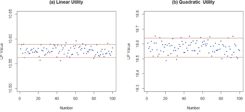
particular distribution, one minimizes the utility function over the interappointments , . . . , . We repeat this 100 times so in total 10 random numbers are needed to get a sample mean, and a sample variance, , of system's cost. Next we illustrate the results of the simulation approach for a system with 11 customers. We assume that the service times of the customers are independent and exponentially distributed (i.i.d.) with parameter 1 for 1,2, . . . , . The results are shown in Fig. 1 and the red line represents z . . We can find that almost all the points appear between two
lines. Therefore, the simulation approach can obtain a UF value which can reflect the performance of schedule well.
4.4 Complexity analysis
Here we discuss the complexity of the proposed heuristic algorithm. First we analyze the procedure of solving subproblem. The complexity of this procedure is 1 . Based on the above, we return to the general procedure of the proposed heuristic algorithm. Its complexity is 1 . Therefore, the complexity of the proposed algorithm is 1 .
Fig. 1. Test for simulation results
5. Numerical experiments
In this section, we will determine the key parameters in SBKSLS and apply the proposed method to a realistic appointment scheduling problems. We will determine the key parameters in Section 5.1. Then in Section 5.2, we will study different distributed service times, e.g., Weibull and lognormal distribution. In Section 5.3 we will apply the proposed method to a real-life example of a CT-scan in a hospital.
5.1 Determine the parameters of SBKSLS
It is necessary to investigate the computing speed (CPU time) of the proposed algorithm. The CPU time is influenced by many aspects, e.g., the number of customers ( ), the amount of customers for the each iteration ( ) and the amount of random numbers in each iteration ( ). However, the first factor is the character of the problem and it is determined by the scale of the instances. Then and are two important parameters in the proposed approach and it needs to find an appropriate combination of and
for the proposed method which can consider both the quality of the solution and the CPU time.
First, we conduct an experiment to determine parameter and the instances are generated which can refer to Vink et al. (2015). We illustrate the results of the proposed method for a system with 11
quadratic utility function with 1 and 0, respectively. For the problem, we solve it with five different (20, 50, 100, 200 and 500) with a given 2 and each instance is solved 10 times. We calculate the average values of the instances as to these combinations ( and ), respectively and the results are shown in Table 1. The first two columns under the parameter category display the values of and , respectively. The rest of Table 1 are divided into two categories: the results for linear utility functions and quadratic utility functions. In each case, the value and CPU time are displayed the resulting average (A), largest (L) and smallest (S) values. The variance of the value ( ) is also displayed.
From Table 1, we observe that the value all have a tendency to decrease with the growth in value and the CPU time has an opposite trend. Besides, the CPU time is acceptable for all instances. Thus, we set 500 for the following experiments because of the best values and the smaller variance for 10 times, which means the value has a better stability.
Second, an experiment is conducted to determine parameter . The instances are generated as the same as the previous experiment and for this problem, we solve it with three different (0, 1 and 2) with a given 500. Table 2 summarizes the results of SBKSLS and the other methods. It is noted that, all the results of lag order approximation method and simulation in this paper are from Vink et al. (2015). We can observe that increasing value reduces the expected total cost of the system. In addition, the results obtained by our proposed method are better than these obtained by lag order approximation method, which is proposed by Vink et al. (2015), on both the objective and the CPU time. When 2, the gap is even smaller than 1% between our results and the optimal results obtained by simulation.
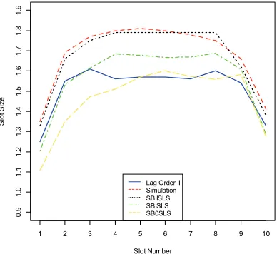
Fig. 2. Optimal lot size for SBKSLS compared with lag order method and simulation with quadratic utility. 11, i.i.d. exponential ( 1) service times
Table 1
Optimization results of SBKSLS with different amount of random numbers for 2 Parameters Linear utility function Quadratic utility function
UF Value Time(seconds) UF Value Time(seconds) AUF LUF SUF AT LT ST AUF LUF SUF AT LT ST 2 20 10.939 11.518 10.668 0.105 7.5 8 6 19.817 23.094 18.346 3.073 7.6 8 7 2 50 10.723 10.946 10.587 0.014 18.6 20 16 19.183 20.472 18.226 0.682 18.1 19 17 2 100 10.676 10.826 10.561 0.007 36.6 38 32 18.619 19.464 18.222 0.121 36.6 38 36 2 200 10.598 10.728 10.550 0.003 75.9 79 74 18.527 18.881 18.304 0.034 73.6 75 72 2 500 10.576 10.684 10.530 0.002 193.1 199 182 18.483 18.685 18.300 0.015 186.9 200 167
1 2 3 4 5 6 7 8 9 10
0.
9
1.
0
1.
1
1
.2
1.
3
1.
4
1.
5
1
.6
1.
7
1.
8
1.
9
Slot Number
Sl
o
t S
iz
e
C. Liu and X. Xiang
Table 2
Optimization results of SBKSLS compared with lag order method and simulation. 11, i.i.d. exponential (CV=1) service times
Method Linear utility functions Quadratic utility functions
UF Value Gap(%) Time(s) UF Value Gap(%) Time(s)
Lag order 0 22.220 111.1 0.12 47.627 160.1 0
Lag order I 12.720 20.8 11 22.918 25.2 26
Lag order II 11.109 5.5 390 19.476 6.4 1200
SB0SLS 11.455 8.8 1 20.656 12.8 1
SBISLS 10.732 2.0 2 18.987 3.7 2
SBIISLS 10.576 0.5 167 18.483 0.9 187
Simulation 10.526 -- 500 18.311 -- 5900
According to above two experiments, we set 2 and 500 for the following experiments. Fig. 2 displays the optimal sizes per arriving customers for different values. We can find that when the value increases the approach results in larger slot sizes. For example, for the first slot (the time between the first and second appointment) the slot size increases from 1.11 based on 0-step look-ahead to a slot size of about 1.35 based on II-steps look-ahead. Furthermore, for the result of II-steps look-ahead, the slots in the middle of the scheme are larger than the slots in the beginning and the end of the scheme. We can also find that the results obtained by II-steps look-ahead is very close to the optimal results which is obtained by simulation method.
5.2 Performance analysis on different distributed service times
In this section, we will study the behavior of different distributed service times, e.g., Weibull and lognormal distribution. According to Cayirli and Veral (2003) service-time distributions have a typical coefficient ranging from 0.35 to 0.85. Given this range, we illustrate our proposed method by using Weibull and lognormal distribution with reasonable coefficient of variations: 0.35, 0.5 and 0.85.
Table 3
Optimization results of SBKSLS compared with lag order method and simulation. 11, i.i.d. Weibull service times
Weibull Linear utility functions Quadratic utility functions
Method UF Value Gap(%) Time(s) UF Value Gap(%) Time(s)
CV=0.35
Lag order 0 5.488 63.3 0 5.168 193.6 0
Lag order I 3.659 8.9 12 2.167 23.1 8
Lag order II 3.435 2.2 640 1.855 5.4 350
SB0SLS 3.746 11.5 0 1.941 10.3 0
SBISLS 3.600 7.1 2 1.777 1.0 3
SBIISLS 3.374 0.4 276 1.764 0.2 274
Simulation 3.360 --- 510 1.760 --- 7700
CV=0.5
Lag order 0 8.808 77.0 0 10.951 188.3 0
Lag order I 5.534 11.2 9 4.689 23.4 17
Lag order II 5.115 2.8 450 4.008 5.5 630
SB0SLS 5.219 4.9 0 4.136 8.9 0
SBISLS 5.076 2.0 2 3.834 0.9 3
SBIISLS 4.984 0.1 297 3.809 0.3 268
Simulation 4.977 --- 500 3.799 --- 9200
CV=0.85
Lag order 0 18.172 104.8 0 33.746 169.4 0
Lag order I 10.489 18.2 23 15.597 24.5 44
Lag order II 9.268 4.5 1800 13.282 6.0 3300
SB0SLS 9.528 7.4 0 13.900 11.0 0
SBISLS 8.994 1.4 2 12.799 2.2 2
SBIISLS 8.905 0.4 278 12.656 1.0 266
In Tables 3 and 4, we display the results of various values to this problem. The results are compared to the lag order method proposed by Vink et al. (2015) and an optimal schedule derived through simulation.
Table 4
Optimization results of SBKSLS compared with lag order method and simulation. 11, i.i.d. lognormal service times
Lognormal Linear utility functions Quadratic utility functions
Method UF Value Gap(%) Time(s) UF Value Gap(%) Time(s)
CV=0.35
Lag order 0 6.537 84.3 0 5.519 173.6 0
Lag order I 4.054 14.3 15 2.507 24.3 12
Lag order II 3.683 3.9 600 2.134 5.8 460
SB0SLS 3.746 5.6 0 2.322 15.1 0
SBISLS 3.606 1.7 1 2.029 0.6 3
SBIISLS 3.559 0.4 33 2.023 0.3 250
Simulation 3.546 --- 460 2.017 --- 7600
CV=0.5
Lag order 0 9.843 91.5 0 11.560 162.7 0
Lag order I 6.020 17.1 15 5.503 25.0 15
Lag order II 5.379 4.7 600 4.683 6.4 370
SB0SLS 5.538 7.8 0 4.876 10.8 0
SBISLS 5.190 1.0 1 4.448 1.1 3
SBIISLS 5.173 0.7 36 4.433 0.7 308
Simulation 5.139 --- 460 4.401 --- 9200
CV=0.85
Lag order 0 17.395 98.1 0 35.064 134.8 0
Lag order I 10.726 22.1 20 18.75 25.6 26
Lag order II 9.372 6.7 670 16.037 7.4 1200
SB0SLS 9.614 9.5 0 16.542 10.8 0
SBISLS 8.860 0.9 1 15.337 2.7 2
SBIISLS 8.841 0.7 28 15.018 0.6 276
Simulation 8.783 --- 590 14.932 --- 7800
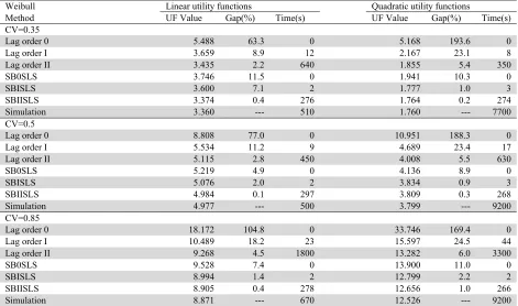
Fig. 3 Optimal lot size for SBKSLS compared with lag order
method and simulation. 11, Weibull distributed service
times with mean 1 and CV=0.5
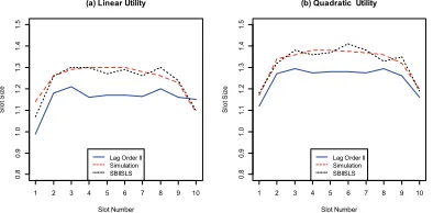
Fig. 4. Optimal lot size for SBKSLS compared with lag
order method and simulation. 11, i.i.d. lognormal
distributed service times with mean 1 and CV=0.5
From the Table 3 and Table 4, we conclude that the application of the proposed method results in a small loss of quality of the appointment schedule. In any case, linear or quadratic utility and either for Weibull or lognormal service-time distribution, our approach with 0 step generates schedules that are no more than 12% from the optimal UF value. Furthermore, from the tables we see that the II-steps look-ahead generates schedules that are reasonably close to the optimal UF value (around 0.1-1.0%). In addition, the computation time is also smaller than that of lag order method for all cases. In Fig. 3 and Fig. 4 we illustrate the schedules derived by the SBKSLS, lag order II method and the simulated optimal in both a Weibull and lognormal setting with coefficient of variation equal to 0.5. We can find that the results
1 2 3 4 5 6 7 8 9 10
0. 8 0. 9 1. 0 1. 1 1. 2 1. 3 1. 4 1. 5
(a) Linear Utility
Slot Number Sl ot S iz e
Lag Order II Simulation SBIISLS
1 2 3 4 5 6 7 8 9 10
0. 8 0. 9 1. 0 1. 1 1. 2 1. 3 1. 4 1. 5
(b) Quadratic Utility
Slot Number Sl ot S iz e
Lag Order II Simulation SBIISLS
1 2 3 4 5 6 7 8 9 10
0 .8 0 .9 1. 01 .1 1 .21 .3 1. 41 .5
(a) Linear Utility
Slot Number
Sl
o
t Si
ze
Lag Order II Simulation SBIISLS
1 2 3 4 5 6 7 8 9 10
0 .8 0 .9 1. 01 .1 1 .21 .3 1. 41 .5
(b) Quadratic Utility
Slot Number
Sl
o
t Si
ze
C. Liu and X. Xiang
obtained by II-steps look-ahead is very close to the optimal results which is obtained by simulation method, which can verify that II-steps look-ahead can obtain an near-optimal solution.
5.3 Application to a CT-scan area
In this section, we consider a real-life scheduling problem in a CT-scan area which refer to Vink et al. (2015), with the following typical parameters: 20, 300(min). As utility function we choose the quadratic loss function with weights 0.75, 0.25 and 1.5. Thus, we have
0.75 0.25 1.5 (12)
We obtained service-time data from the Deventer Hospital described in De Mast et al. (2011). The best fit to this data results in a lognormal distribution with scale parameter 2.4 and location parameter
0.58. The coefficient of variation is 0.63.
Table 5
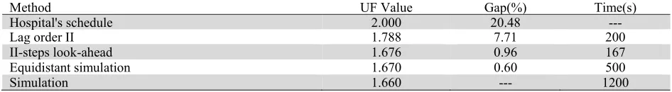
The schedule results for a CT-scan
Method UF Value Gap(%) Time(s)
Hospital's schedule 2.000 20.48
---Lag order II 1.788 7.71 200
II-steps look-ahead 1.676 0.96 167
Equidistant simulation 1.670 0.60 500
Simulation 1.660 --- 1200
In order to compare our method, we state several approximation approaches in Table 5. The table includes the hospital's current schedule and the simulated optimal schedule. For each approach in our study the table reports the values of the utility function, the difference between the values of the approach and that of the simulated optimal value, and the computer's CPU time of the simulation study.
We observe that, given the utility function, the current schedule differs about 20% compared to the simulated optimal value of the , that is, the total loss of the system. Also, we see that the lag order II differs about 7.71% from the optimal simulated outcome of the . But for the II-steps look-ahead method, the gap is only 0.96%. The advantage of II-steps look-ahead method is that it significantly gains in computation time compared to the simulated optimal value. Finally, we observe that an equidistant approximation method gets close to the simulated optimal results, but it takes our computer 3 times more CPU effort to get to these results.
6. Conclusions
In this paper we have studied the problem of appointment scheduling of customers with a finite planning horizon. The customers are punctual and can be considered as jobs having random service times. However, no-shows and walk-in customers are not allowed. We have developed a SBKSLS that minimizes a function of the waiting time of the customers, the idle time of the server, and the lateness of the schedule. The proposed method with I-step look-ahead yields near-optimal schedules (about 2% from the optimal utility value level) within sufficiently smaller computation times. The II-steps look-ahead method yields schedules that are smaller than 1% from the optimal value, and is faster than simulations.
of these issues cannot be dealt with in a straightforward manner and require new models. From a more algorithmic perspective, it would be interesting to investigate how SBKSLS can improve existing heuristics when combined.
References
Bailey, N. T. (1952). A study of queues and appointment systems in hospital out-patient departments, with special reference to waiting-times. Journal of the Royal Statistical Society. Series B (Methodological), 14(2), 185-199.
Begen, M. A., & Queyranne, M. (2011). Appointment scheduling with discrete random durations.
Mathematics of Operations Research, 36(2), 240-257.
Begen, M. A., Levi, R., & Queyranne, M. (2012). Technical note-a sampling-based approach to appointment scheduling. Operations Research, 60(3), 675-681.
Bendavid, I., & Golany, B. (2011). Setting gates for activities in the stochastic project scheduling problem through the cross entropy methodology. Annals of Operations Research, 189(1), 25-42. Cayirli, T., & Veral, E. (2003). Outpatient scheduling in health care: a review of literature. Production
and Operations Management, 12(4), 519-549.
Chakraborty, S., Muthuraman, K., & Lawley, M. (2010). Sequential clinical scheduling with patient no-shows and general service time distributions. IIE Transactions, 42(5), 354-366.
Denton, B., & Gupta, D. (2003). A sequential bounding approach for optimal appointment scheduling.
IIE transactions, 35(11), 1003-1016.
De Mast, J., Kemper, B., Does, R., Mandjes, M., & Van der Bijl, H. (2011). Process improvement in healthcare: Overall resource efficiency. Quality and Reliability Engineering International, 27(8), 1095-1106.
Gupta, D., & Denton, B. (2008). Appointment scheduling in health care: Challenges and opportunities.
IIE transactions, 40(9), 800-819.
Kemper, B., Klaassen, C. A., & Mandjes, M. (2014). Optimized appointment scheduling. European Journal of Operational Research, 239(1), 243-255.
Kuiper, A., Kemper, B., & Mandjes, M. (2015). A Computational approach to optimized appointment scheduling. Queueing Systems, 79(1), 5-36
Mancilla, C., & Storer, R. (2012). A sample average approximation approach to stochastic appointment sequencing and scheduling. IIE Transactions, 44(8), 655-670.
Mak, H. Y., Rong, Y., & Zhang, J. (2014). Appointment scheduling with limited distributional information. Management Science, 61(2), 316-334.
Robinson, L. W., & Chen, R. R. (2003). Scheduling doctors’ appointments: optimal and empirically-based heuristic policies. IIE Transactions, 35(3), 295-307.
Vink, W., Kuiper, A., Kemper, B., & Bhulai, S. (2015). Optimal appointment scheduling in continuous time: The lag order approximation method. European Journal of Operational Research, 240(1), 213-219.
Wang, P. P. (1997). Optimally scheduling N customer arrival times for a single-server system. Computers & Operations Research, 24(8), 703-716.
Wang, P. P. (1999). Sequencing and scheduling N customers for a stochastic server. European Journal of Operational Research, 119(3), 729-738.
Weiss, E. N. (1990). Models for determining estimated start times and case orderings in hospital operating rooms. IIE transactions, 22(2), 143-150.