Comparison of Some Iterative Methods of Solving Nonlinear Equations

http://www.sciencepublishinggroup.com/j/ijtam doi: 10.11648/j.ijtam.20180402.11

ISSN: 2575-5072 (Print); ISSN: 2575-5080 (Online)

Comparison of Some Iterative Methods of Solving

Nonlinear Equations

Okorie Charity Ebelechukwu, Ben Obakpo Johnson, Ali Inalegwu Michael, Akuji Terhemba Fidelis

Department of Mathematics and Statistics, Faculty of Pure and Applied Sciences, Federal University, Wukari, Nigeria

Email address:

To cite this article:

Okorie Charity Ebelechukwu, Ben Obakpo Johnson, Ali Inalegwu Michael, Akuji Terhemba Fidelis. Comparison of Some Iterative Methods of Solving Nonlinear Equations. International Journal of Theoretical and Applied Mathematics. Vol. 4, No. 2, 2018, pp. 22-28.

doi: 10.11648/j.ijtam.20180402.11

Received: December 23, 2017; Accepted: May 15, 2018; Published: July 26, 2018

Abstract:

This work focuses on nonlinear equation (x) = 0, it is noted that no or little attention is given to nonlinear equations. The purpose of this work is to determine the best method of solving nonlinear equations. The work outlined four methods of solving nonlinear equations. Unlike linear equations, most nonlinear equations cannot be solved in finite number of steps. Iterative methods are being used to solve nonlinear equations. The cost of solving nonlinear equations problems depend on both the cost per iteration and the number of iterations required. Derivations of each of the methods were obtained. An example was illustrated to show the results of all the four methods and the results were collected, tabulated and analyzed in terms of their errors and convergence respectively. The results were also presented in form of graphs. The implication is that the higher the rate of convergence determines how fast it will get to the approximate root or solution of the equation. Thus, it was recommended that the Newton’s method is the best method of solving the nonlinear equation f(x) = 0 containing one variable because of its high rate of convergence.

Keywords:

Nonlinear, Iterative Methods, Convergence, Variable

1. Introduction

Numerical methods are used to provide constructive solutions to problems involving nonlinear equations. A nonlinear equation may have a single root or multiple roots.

This research work will make emphasis on solving nonlinear equation in one dimension and involving one unknown, : → which has scalar X as solution, such that

0.

The study of this work cannot be discussed at peak without first making necessary attempts to discuss the branch of mathematics that it arises from which is numerical analysis.

Numerical analysis, is an area of mathematics and computer science that creates, analyses and implement algorithm for obtaining numerical solutions to problems involving continuous variables. Numerical algorithms are at least as old as the Egyptian Rhind papyrus (1650 BC) which describes a root finding for solving a simple equation like nonlinear equations in general, a problem that requires the determination of values of unknowns x x1, 2...xnfor which

(

1, 2,...,

)

0

k n

f x x x = , k=1,2,…n (Encyclopedia.com). Nonlinear equations are equations whose graphsolution does not form a straight line. In a nonlinear equation, the variables are either of degree greater than one or less than one or less than but never one. (Mathematics dictionary) An equation which when plotted on a graph does not trace a straight line but a curve is called nonlinear equation (www.Business dictionary.com).

Nonlinear equations are solved by iterative methods. A trial solution is assumed, the trial solution is substituted into the nonlinear equation to determine the error, or mismatch, and the mismatch is used in some systematic manner to generate an improved estimate of the solution. Several methods for finding the roots of nonlinear equations exist. Such methods of choice for solving nonlinear equations are Newton’s method, the secant method etc.

involving more complicated terms such as trigonometric, hyperbolic, exponential or logarithmic functions are referred to as transcendental equations. This in general is referred as nonlinear equations. [5] It is well known that when the Jacobian of nonlinear systems is nonsingular in the neighborhood of the solution, the convergence of Newton method is guaranteed and the rate is quadratic. Violating this condition, i.e. the Jacobian to be singular, the convergence may be unsatisfactory and may even be lost [1].

If f x

( )

is a polynomial of degree two or three or four, exact formulae are available. But, if f x

( )

is a transcendental function like a be+ x+sinx d+ logx etc. The solution is not exact when the coefficient is numerical values, it can adopt various numerical approximate methods to solve such algebraic and transcendental equations. [7], professor of mathematics (Rtd) P.S.G College of technology Coimbatore. Systems of nonlinear equations are difficult to solve in general. The best way to solve these equations is by iterative methods. One of the classical methods to solve the system of nonlinear equations is Newton method which has second order rate of convergence. This speed is low when we compare to third order method. [9]. Many of the complex problems in science and engineering contain the function of nonlinear and transcendental nature in the equation of the form f x

( )

=0. Numerical methods like Newton’s method are often used to obtain the approximate solution of such problems because it is not always possible to obtain its exact solution by usual algebraic process [8].

1.1. Statement of Problem

Nonlinear equations are approximately one of the difficult equations in sciences and less attention is given to them compared to the other forms of equations.

1.2. Aim and Objectives of the Study

The aim of this study is to determine the method that is the best in solving nonlinear equations using numerical methods

The following are the objectives of the study;

i. Determining the existence of a solution, convergence and errors of the methods;

ii.Comparing the stated methods to determine the most appropriate method or methods for the given equation.

2. Materials and Methods

For the purpose of this work, the following methods were compared; Newton method, secant method, the regular falsi method and the bisection method.

2.1. Newton Method

Newton method is one of the most popular numerical method is often referred as the most powerful method that is used to solve for the equation f(x) =0, where f is assumed to have a continuous derivative f ' . This method originated

from the Taylor’s series expansion of the function f x

( )

about the pointx₁, such that

( ) ( ) (

) ( )

(

)

2

( )

1 1 1 1 1

1

' ''

2!

f x −f x + x−x f x + x−x f x + (1)

Where f and its first and second derivative f ' and f '' are calculated at x1. Taking the first two terms of the Taylor’s

series expansion, We have

( )

( ) (

1 1

) ( )

' 1

f x = f x + −x x f x (2)

We then set (1) to zero (i.e.f x

( )

=0) to find the root of the equation which yields

( ) (

1 1

) ( )

' 1 0

f x + −x x f x = (3)

Rearranging (3) above, we obtain the next approximation to the root, given rise to

( )

( )

1

1 1

'

f x

x x

f x

= − (4)

Thus generalizing (4) we obtain the Newton iterative method

( )

( )

1

'

k

k k

k f x

x x

f x

+ = − , where k Є N (5)

Example: f( ) = 3+ -1=0

Apply Newton’s method to the equation. correct to five decimal places.

F (0) = -1, f(1)= 1, therefore the root lies between 0 and 1.

( )

( )

1

'

k

k k

k f x

x x

f x

+ = −

( )

2

' 3 1

f x = x +

( )

( )

3

1 ₂

1

' 3 1

k k k

k k k

k k

f x x x

x x x

f x x

+ = − = − + −

+

Solving the right hand side yields

3

1 ₂

1 3 1

k k

k k

k

x x

x x

x

+ = − + −₊

Convergence of Newton’s Method Here in Newton’s method

( )

( )

1

'

k

k k

k f x

x x

f x

+ = −

k+1 = Ø ( k) and Ø ( k) = k -

( )

( )

' k k f x

f x .

Hence the equation is

= Ø ( ) where Ø ( ) = -

( )

( )

' k k f x f x

The sequence 1, 2, 3... converges to the exact value if |

Ø׀( ) | < 1

i.e. if

( )

( )

( )

2 2 ' '' 1 1 '

f x f x

f x  ₋      − <     (6)

i.e. if

( )

( )

( )

2

''

1 '

f x f x

f x

<

 

 

This implies that Newton method converges if

( ) ( )

( )

2

'' '

f x f x <_f x _

2.2. Secant Method

The secant method is just a variation from the Newton’s method. The Newton method of solving a nonlinear equation

( )

0

f x = is given by the iterative formula.

( )

( )

1 ' k k k k f x x x f x

+ = − (7)

One of the drawbacks of the Newton’s method is that one have to evaluation the derivative of the function. To overcome these drawbacks, the derivative of the function

( )

f x is approximated as

( )

( ) (

1

)

1

' k k k

k k

f x f x

f x x x − − − =

− (8)

Substituting equation (8) into (7)

( )

( )

( ) ( )

1

1

1

k k k k

k k

k k

x f x x f x

x x

f x f x

− + − − = − −

By factoring out f

( )(

)

( ) ( )

1

1

1

k k k

k k

k k

f x x x

x x

f x f x

− +

−

−

= −

− (9)

This can also be written as

( ) ( ) ( )

1

1

1

k k

k k k

k k

x x

x x f x

f x f x

− + −  ₋  = −  −    

The above equation is called the secant method. This method requires two initial guess.

Example: Solve the equation f x

( )

= x3+ −x 1 using secant method. Correct to five decimal places.

Solution,

( )

0 1,

f = − f

( )

1 =1

The root lies between 0 and 1and taking x₀=1 and x₁=1

By secant method, first approximation is when k = 1;

( )

(

)

( )

1 1

( )

0

2 1

1 0

f x x x

x x

f x f x

− = −

−

When k = 2;

( )(

)

( ) ( )

2 2 1

3 2

2 1

f x x x

x x

f x f x

−

= −

−

When k =3;

( )(

)

( ) ( )

3 3 2

4 3

3 2

f x x x

x x

f x f x

− = −

−

When k = 4;

( )(

)

( )

4 4

( )

3

5 4

4 3

f x x x

x x

f x f x

−

= −

−

When k =5;

( )(

)

( ) ( )

5 5 4

6 5

5 4

f x x x

x x

f x f x

− = −

−

When k = 6;

( )(

)

( ) ( )

6 6 5

7 6

6 5

f x x x

x x

f x f x

− = −

−

When k = 7;

( )(

)

( ) ( )

7 7 6

8 7

7 6

f x x x

x x

f x f x

−

= −

−

When k = 8;

( )(

)

( ) ( )

8 8 7

9 8

8 7

f x x x

x x

f x f x

 ₋ 

= − 

−

 

 

When k = 9;

( )(

)

( ) ( )

9 9 8

10 9

9 8

f x x x

x x

f x f x

 ₋ 

= − 

−

 

 

When k =10;

( )(

)

( ) ( )

10 10 9

11 10

10 9

f x x x

x x

f x f x

 ₋ 

= − 

−

 

 

Convergence of Secant Method

Say x_k = +α e x_{k, k+1}= +α e_k+1 (10)

Where

α

=root of f x

( )

=0

1

, k k

e e₊ , are errors

k

x =approximationat k iteration

1

k

x₊ =approximationof

α

at k+1

α

=root of f(x) = 0

If e_k+1=Ne_kpwhere N is a constant

Then the rate of convergence of the method is

( )

( )( )

( ) ( )

(

1 1

)

1

1

1

k k k k

k

k k

f x x f x x

x

f x f x

− − −

+

−

−

− (11)

( )(

)

( ) ( )

11

k k k k

k k

f x x x

x

f x f x

−

−

−

= −

Say f

( )

α

=0 and i.e error in the kth iteration

(

)

k k

e =

α

−x x_k+1=e_k+1+

α

k

x = +e

α

1 1

k k

x ₋ =e₋ +

α

(13)

All the above is named (13) Using (13) in (12)

( ) (

)

( ) (

)

1 1

1

1

k k k k

k

k k

e f x f x e

e

f x f x

− −

+

−

− =

− (14)

By mean value theorem there exist

ω

in the interval xk

and

α

such that

( )

( ) ( )

' k

k

f x f

f

x α ω

α − =

− (15)

We get '

( )

( )

k

k

f x f

e

ω =

i.e f x

( )

_k =e f_k '

( )

ω

(16)

Using (13), we get

( )

(

)

( ) ( )

1

1 1

1

' _k ' _k

k k k

k k

f f

e e e

f x f x

ω

ω

−

+ −

−

− =

− (17)

This gives the convergence.

2.3. Regular Falsi Method

This method is also being called the method of false position.

Consider the equation f x

( )

=0 and let f a

( )

and f b

( )

be of opposite signs. Also, let a < b.

The curvey= f x

( )

will meet the - axis at some point between A (a,f a

( )

) and B (b f b

( )

). The equation of the chord joining the two points A (a, f a

( )

and B (b, f b

( )

) is

( )

( ) ( )

y f a f a f b

x a a b

− −

=

− − (18)

The -coordinate of the point of intersection of this chord for the root of - axis gives an approximate value for the root off x

( )

=0, setting y = 0 in the chord equation, we get

( )

( ) ( )

f a f a f b

x a a b

− −

=

− −

( ) ( )

( )

( )

( )

( )

x f a_ − f b _−af a +af b = −af a +bf a

( ) ( )

( )

( )

x f a_ − f b _=bf a −af a

Therefore,

( )

( )

( ) ( )

af b bf a x

f b f a

− =

− (19)

The value of 1 gives an approximate value of the roots of

( )

f x = 0, (a< 1<b).

Now f x

( )

₁ and f a

( )

are of opposite signs or f x

( )

₁ and

( )

f b are of opposite sign.

If f x

( )

₁ . f a

( )

< 0, then 2 lies between 1 and a

Hence

( )

( )

( ) ( )

1 1

2

1

af fx x f a

x

f x f a

− =

−

In the same way we get 3, 4...

The general formula is

( )

( )

( ) ( )

1

k

af b bf a x

f b f a

+ = ₋− (20)

Example: Solve the equation f x

( )

= x3+ −x 1 using regular falsi method, correct to five decimal places

Solution

( )

( )

( ) ( )

1

k

af b bf a

x

f b f a

+ = −₋

When k = 0,

a

=

0,

b

=

1

( ) ( )

1

0 1 1 1 1

0.5

1 1 2

x = − − = =

+

( )

1 0.375 f x = −

When k =1

A root lies between0.5 and 1 such that a=0.5 and b=1etc. Convergence of Regular Falsi Method

If x_k be the sequence of approximations obtained from

(

)

( ) (

1

) ( )

1

1

k k

k k k

k k

x x

x x f x

f x f x

− +

−

−

= −

− (21)

And α be the exact value of the root of the equation f(x) = 0, then

1 1

k k

x

₊

= +

α

e

₊

Wheree_k+1 being the error involved in the

(

k+1

)

th

approximation. Hence (21) gives,

(

)

(

) (

) (

)

(

)

(

)

(

) (

)

1 1

1

1 1

1

1

=

k k

k k k

k k

k k k k

k

k k

e e

e e f e

f e f e

e f e e f e

e

f e f e

α α α

α α

α α

α α

− +

−

− −

+

−

−

+ = + − +

+ − +

+ − +

=

( )

( )

( )

( )

( )

( )

( )

( )

( )

( )

( )

( )

(

) ( )

(

) ( )

(

) ( ) (

)(

)

2 2

1

1 1

2 2

1 1

1

1 1

1 1

1

' '' .... ' '' ...

2! 2!

' '' ... ' '' ...

2! 2!

'' ... 2!

=

' '

2!

k k

k k k k

k k

k k

k k

k k k k

k k k k

k k

e e

e f e f f e f e f f

e e

f e f f f e f f

e e

e e f e e f

e e e e

e e f f

α α α α α α

α α α α α α

α α

α

−

− −

− −

−

− −

− −

−

   

+ + + − + + +

   

   

   

   

+ + + − + + +

   

   

   

− + − +

− +

− +

( )

( )

( )

( )

1

1

' ...

'' ... 2

=

' '' ...

2

k

k k

e f

e e

f f

α

α

α α

−

−

+

+ +

 

+  +

 

Therefore f(x) =0

2.4. Bisection Method

Suppose we have an equation of the formf x

( )

= 0 whose solution is in the range (a, b) is to be determined. We also assume that f x

( )

is continuous and it can be algebraic or transcendental. If f a

( )

and f b

( )

are of opposite signs, then at least one root exist between a and b.

As a first approximation, we assume that root to be x0 =

(mid point of the ends of the range).

Now, find the sign of f x

( )

0 . If f x

( )

0 is negative, the root lies between x0 and b. Any one of this is true.

This solution is found by repeated bisection of the interval and in each iteration picking that half which also satisfies that sign condition. The number of iteration required may be

determined from the relation 2k b− ≤a

€

The general formula is

2

k

a b

x = + (23)

Example: Solving the equation f x

( )

= x3+ −x 1_{, correct}

to five decimal places.Using bisection method f x

( )

= 3

1

x + −x ,correct to five decimal places.

Solution

2

k

a b

x = +

When k =0

A root lies between 0 and 1 such that a = 0 and b = 1 Convergence of Bisection Method

The successive approximation xk of a root x=

α

of the

equation f x

( )

=0 is said to converge to x=

α

with order

1

q

≥

If xk+1− ≤

α

c xk−

α

Here q k, >0, k and c is some constants greater than 0 When q=1 and 0<c<1, then the convergence is said to be of first order and c is called the rate of convergence.

3. Results

Following the example f x

( )

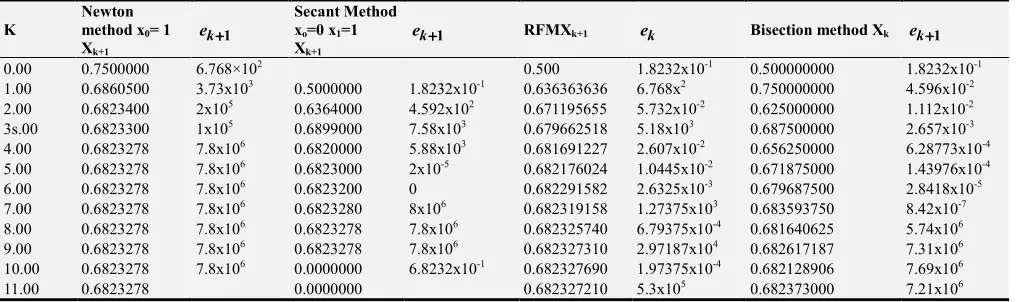
=x3+ −x 1of the nonlinear equation and illustrating the results by the four methods of solving nonlinear equations f(x)= 0 in this work, the results of the methods are presented in the graphs and table below.

Table 1. The Results of the four methods.

K

Newton method x0= 1

Xk+1

1

k

e ₊₊₊₊

Secant Method xo=0 x1=1

Xk+1

1

k

e ₊₊₊₊ RFMXk+1 e_k Bisection method Xk e_k++++₁

0.00 0.7500000 6.768×102 _{0.500 1.8232x10}-1 _{0.500000000 1.8232x10}-1

1.00 0.6860500 3.73x103 _{0.5000000 1.8232x10}-1 _{0.636363636 6.768x}2 _{0.750000000 4.596x10}-2 2.00 0.6823400 2x105 _{0.6364000 4.592x10}2 _{0.671195655 5.732x10}-2 _{0.625000000 1.112x10}-2 3s.00 0.6823300 1x105 _{0.6899000 7.58x10}3 _{0.679662518 5.18x10}3 _{0.687500000 2.657x10}-3 4.00 0.6823278 7.8x106 _{0.6820000 5.88x10}3 _{0.681691227 2.607x10}-2 _{0.656250000 6.28773x10}-4 5.00 0.6823278 7.8x106 _{0.6823000 2x10}-5 _{0.682176024 1.0445x10}-2 _{0.671875000 1.43976x10}-4

6.00 0.6823278 7.8x106 _{0.6823200 0 0.682291582 2.6325x10}-3 _{0.679687500 2.8418x10}-5

7.00 0.6823278 7.8x106 _{0.6823280 8x10}6 _{0.682319158 1.27375x10}3 _{0.683593750 8.42x10}-7 8.00 0.6823278 7.8x106 _{0.6823278 7.8x10}6 _{0.682325740 6.79375x10}-4 _{0.681640625 5.74x10}6 9.00 0.6823278 7.8x106 _{0.6823278 7.8x10}6 _{0.682327310 2.97187x10}4 _{0.682617187 7.31x10}6 10.00 0.6823278 7.8x106 _{0.0000000 6.8232x10}-1 _{0.682327690 1.97375x10}-4 _{0.682128906 7.69x10}6

K

Newton method x0= 1

Xk+1

1

k

e ₊₊₊₊

Secant Method xo=0 x1=1

Xk+1

1

k

e ₊₊₊₊ RFMXk+1 e_k Bisection method Xk e_k++++₁

12.00 0.6823278 0.0000000 0.682327551 6.905x10-5 0.682250950 7.551x106

13.00 0.6823278 0.0000000 0.682327743 8.02x10-6 _{0.682311980 7.743x10}6

14.00 0.6823278 0.0000000 0.682327497 2.25x105 _{0.682342500 7.497x10}6

15.00 0.6823278 0.0000000 0.682327730 7.4x106 0.682327400 7.73x106

16.00 0.6823278 0.0000000 0.682327785 1.487x105 _0.682334870

17.00 0.6823278 0.0000000 0.682327799 1.1x105 _0.682331000

18.00 0.6823278 0.0000000 0.682327802 9.12x106 0.682329120

19.00 0.6823278 0.0000000 0.682327803 8.18x106 _0.682328180

20.00 0.6823278 0.0000000 0.682327030 7.71x106 _0.682327710

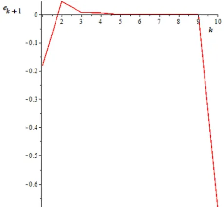
Figure 1. The graph of Newton method.

The error in each kth iteration in the Newton Method converges positively and remains positive with great speed and accuracy throughout the value of k.

Figure 2. The graph of Secant method.

The errors in the Secantmethod alternate, this means that the errors moves from positive to negative but remains stable at the point of convergence but also diverges at a point.

Figure 3. The graph of Regular falsi method.

In the regular falsi method the error in each kth iteration converges negatively but turn positive at the point of convergence and remains positive throughout the value of k.

The error in kth iteration of the bisection method is alternative, this implies that it changes from positive to negative but remains positive at the point of convergence.

The table above compared the results of all the four methods combined and Newton method was found to be the best method because of its fast and accurate convergence to the roots, the Secant method also shows a high and speedy convergence but the method is due to fail at any time or perhaps diverge to another solution i.e. whenever x_k+1=x_k. The regular falsi method also shows a level of speedy convergence but not as compared to the Newton and secant methods respectively but certainly above the bisection method. The Bisection method has the slowest convergence to the roots than any of the other three methods but its convergence to the root is sure no matter the number of iterations. After comparing all the four methods it will be safe to say that the rate of one iteration of the Newton method is equivalent to four iterations of the bisection method.

4. Discussion

Iterative method is one in which we start from an approximation to the true solution and if successful, obtain better approximation from a computational cycle repeated as often as necessary for achieving a required accuracy, so that the amount of arithmetic depends upon the accuracy required.

It also shows the rate of convergence, with regard to convergence, we can summarize that a numerical method with a higher rate of convergence may reach the solution of the equation with less iterations in comparison to another method with a slower convergence.

The existence of a solution of a nonlinear equation

( )

0

f x = with one variable is determined by the intermediate value theorem.

From the methods explained in this work, it can be discovered that the Newton method is the best iterative method for solving the nonlinear equations with one variable as it converges more rapidly and accurately to the root of the equation when the initial guess is close to the roots of the equation.

It is also clear to say that for secant, at any given time before it converges to the root of the equation where

1 ,

k k

x ₊ =x then it means that the method will fail from that point.

The regular Falsi method converges more slowly compare to the Newton and secant method respectively and the bisection method requires a large number of iterations before it converges to the root of the equationirrespective of how one starts close to the roots of the equation.

5. Conclusion

From the methods tested, the Newton method appeared to be the most robust and capable method of solving the nonlinear equation f x

( )

=0.Results obtained from the four methods above show that the Newton Method is the most efficient method in finding the roots of non-linear equations seeing that it converges to the roots of the non-linear equation faster than the other three methods. That is it converges after a few iterations unlike the other three methods which converges after many iterations.

References

[1] Aisha H.A; Fatima W.L; Waziri M.Y. (2014). International journal of computer application, vol 98business dictionary. (2016). www.Business dictionary.com. copyright 2001-2016, web finance, In

[2] Dass H.K. and Rajnish Verma (2012).Higher Engineering Mathematics. Published by S. Chand and Company ltd (AN ISO 90012008 Company). Ram New Delhi- 110055.

[3] Deborah Dent and Marcin Paaprzycki. (2000).Recent advances in solvers for nonlinear algebraic Equations. School of mathematical sciences, University of Southern Mississippi Hattiesburg.

[4] Erwin Kreysig (2011). Advance Engineering Mathematics. Tenth edition. Published by John Wileyand sons, inc.

[5] Free dictionary. (2011). American Heritage dictionary of the English language, fifth edition, copyright by Houghton Mifflin Harcourt publishing company.

[6] Giberto E. Urroz. (2004).Solution of nonlinear equations. A paper document on solving nonlinearequation using Matlab. [7] John Rice (1969), Approximation of functions: Nonlinear and

Multivariate Theory, Publisher; Addison–Wesley Publishing Company.

[8] Kandasamy P. (2012). Numerical methods. Published by S. Chand and company ltd (AN ISO 9001; 2000 Company). Ram Nagar, new-Delhi – 110 055

[9] Masoud Allame. (2001). A new method for solving nonlinear equations by Taylor’s Expansion. Conference paper, Islamic Azad University. Numerical analysis Encyclopedia Britannica online. <www.britannica/com/topic/numerical analysis >. [10] Sara T.M. Suleiman. (2009).Solving Nonlinear equations

using methods in the Halley class. Thesis for the degree of master of sciences.