Multi-objective linear mathematical programming for solving U-shaped robotic assembly line balancing

(1)

Multi-Objective Linear Mathematical Programming for Solving U-Shaped

Robotic Assembly Line Balancing

M. Rabbani 1,_{, A. H. Khezri}1_{, H. Farrokhi-Asl}2_{, S. Aghamohamadi-Bosjin}1

1 _{Department of Industrial Engineering, College of Engineering, University of Tehran, Tehran, Iran.} 2 _{Department of Industrial Engineering, Iran University of Science and Technology, Tehran, Iran.}

A B S T R A C T

In recent years, robots have been an eminent solution for manufacturers to facilitate their process and focus on a variety of their products. As the importance of robot usages, our paper focuses on the robotics assembly line. In this paper, we have considered the cycle time, robot operational costs, robot purchase costs, and robot energy consumptions. In the following, we add robot failure rates to have an efficient and high-quality assembly line. The presented model is a multi-objective problem, therefore, the linear programming methods as goal programming and augmented ε-constraint method are applied to optimize the problem. In the end, we have considered a case study to examine and show the applicability of the proposed model on the real situation.

Keywords:Robotic mixed-model assembly line balancing (RMALB), U-shaped assembly line, Multi-objective optimization, Goal programming, Augmented ε-constraint method.

Article history: Received: 07 October 2018 Revised: 22 January 2019 Accepted: 26 February 2019

1. Introduction

Nowadays, the competitive market leads companies to promote their manufacturing systems by more flexible and effective plan. The plan should satisfy quickly and efficiently the manufacture’s demands. Due to the importance of the production plan, it was an important and controversial issue in the past decades. For the first time, Henry Ford introduced the manufacturing assembly line. Over the past years, Assembly Line Balancing (ALB) has had an eminent impact on the manufacturing systems. ALB is an ordering of a sequence stations, linked together by a transport system. Each station operates one or more tasks on the partially finished product. Based on product verity, there exist three types of assembly lines [1]:

_{Corresponding author}

E-mail address: [email protected] DOI:10.22105/riej.2018.128451.1040

International Journal of Research in Industrial

Engineering

(2)

Rabbaniet al. / Int. J. Res. Ind. Eng 8(1) (2019) 1-16 2

 Single-Model Lines: In large quantities, only one homogeneous product is continuously produced.

 Mixed-Model Lines: On the same line in an arbitrarily inter-mixed sequence, several models of a basic product are produced.

 Multi-Model Lines: In separately batches family of products which present significant differences in processes are produced on one or more assembly lines.

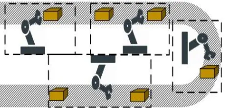
Figure 1. Shapes of straight, U-shaped, and multi-model lines.

(3)

3 Multi-objective linear mathematical programming for solving u-shaped robotic assembly line balancing

Because of the advantages and extensively uses of robots in assembly line, in this paper we have considered the Robotic Assembly Line Balancing (RALB). In the recent years, the high flexibility of robots, high productivity, and ability for production of high quality products, made robots the most prominent tools to develop the production plan. The RALB problem is the way of getting an optimal assignment to the robotic stations and selecting the best-fit robots to operate the tasks [12], and was first described by [13]. Three major objective functions are considered in RALB problem including the minimizing number of workstations (RALB-I), minimizing cycle time (RALB-II), minimizing energy consumption, and maximizing efficiency. The [14] formulated the problem for minimizing the number of workstations for a given cycle time subject to allocating of tasks to work stations. Later, the [15] extended that problem used an exact branch and bound algorithm. Also, the [16] developed an exact branch and bound algorithm.

To gain more profit and product verity of products, manufacture needs to have more flexibility with today’s demanding market. In this case, the mixed-model assembly lines designed, and allowed manufacture to product a group of similar model items and provide more flexibility in producing according to market demand. Many articles have worked on the mixed-model ALBP [17- 22]. On the other hand, a few researches have focused on Robotic Mixed-Model Assembly Line Balancing (RMALB) problem. The [23] developed a mathematical model for two-sided RMALBP to minimize the cycle time respect to robot set-up and sequence-dependent set-up times. The [24] present a mathematical model for U-shaped line with considering minimizing cycle times, robot purchasing, robot set-up, sequence-dependent set-up costs. In this model, they considered two assumptions: Two or more robots can operate the work at the same station. In addition, tasks in line were handled by two groups: 1) the special tasks can be performed in one model, 2) the common tasks can be performed in several models. The [25] developed a new efficient heuristic algorithm based on beam search in order to minimize the sum of cycle times over all models.

(4)

2. Problem Description

The problem is a multi-objective type II Robotic Mixed-Model Assembly Line Balancing (RMALB-II). Based on the previous researches by [24], we have developed a new model consists of robotic operational costs and energy consumptions. In this model, we are into finding an optimal or near optimal configuration of task, workstations, and robot by considering the goals including minimization of the cycle time, robot's operational energy consumption, robots operational, and purchasing costs. Because of flexibility and adaptability of the U-shaped line, we consider it as our production line. This system allows forward and backward assignment to be performed, so the robot can move less between workstations and logically the cycle time, energy consumption, and other cost could be decreased [24, 33, 34]. To product M types of product, the U-line of assembly has J workstations with a robot in each and it has I tasks of invisible assembly task [28]. Before introducing the model, based on [28], [27], and [35] some basic assumptions considered in this paper are provided as follows:

Power consumption of each robot is assumed and energy consumption is computed with the power consumption of each robot.

Assembly tasks cannot be subdivided. The precedence relations among the activities are distinctive and constant. Precedence graph represented this precedence.

The processing time of an assembly task relies on the assigned robot type that the duration of an activity by a robot is deterministic.

Setup times between tasks are deterministic, depend on the assigned robot, and are independent of the assigned workstation.

The line is balanced for multiple products. Products are models in U-shaped line.

The purchase cost of each type robots is considered.

The time of setup for task and robot setup times are considered.

There are 𝑟 types of robot available (𝑟 ≥ 1) that there is no restriction on the number of robots available.

The travel times of operators are ignored.

Material handling, loading and unloading times are insignificant, so they are contained in processing times.

(5)

2.1 Mathematical Modeling

Indices

𝑖 Number of assembly tasks; 𝑖 = 1, 2, … , 𝐼.

𝑗 Number of workstations; 𝑗 = 1, 2, … , 𝐽.

𝑚 Number of product model; 𝑚 = 1, 2, … , 𝑀.

𝑟 Number of robot types; 𝑟 = 1, 2, … , 𝑅.

Parameters

𝑝𝑟𝑡(𝑖) Set of immediate predecessors of task 𝑖.

𝑃𝐶𝑟 Cost of a robot type 𝑟,to be purchased.

𝑆𝑒𝐶𝑟𝑖 Setup cost of a robot of type 𝑟, for processing task 𝑖.

𝑆𝑑𝐶𝑖 Sequence dependent setup cost for processing task 𝑖.

𝑆𝑒𝑇𝑖𝑟 Setup time of a robot of type 𝑟, for processing task 𝑖.

𝑆𝑑𝑇𝑖 Sequence dependent setup time for processing task 𝑖.

𝑃𝑇𝑖𝑚𝑟 Processing time of task 𝑖for model 𝑚 by robot 𝑟.

𝑂𝐸𝐶𝑟 Operation energy consumption of the robot 𝑟 per time unit.

𝑆𝐸𝐶𝑟 Standby energy consumption of the robot 𝑟 per time unit.

𝐿𝑅𝑟 Maximum length of a robot of type 𝑟.

𝑊𝑅𝑟 Maximum width of a robot of type 𝑟.

𝐿𝑊𝑗 Minimum length of a workstation .

𝑊𝑊𝑗 Minimum width of a workstation 𝑗.

𝐶𝑇𝑚𝑎𝑥 Maximum station time among all stations.

(6)

Considered objective functions are given as below:

𝑀𝑖𝑛 𝐶𝑇 = ∑ 𝐶𝑇𝑚 𝑀 𝑚=1 (1) 𝑀𝑖𝑛 𝑅𝑂𝐶 = (∑ ∑ ∑ ∑ 𝑆𝑒𝐶𝑟𝑖 𝑅 𝑟=1 𝑀 𝑚=1 𝐽 𝑗=1 𝐼 𝑖=1 + ∑ ∑ ∑ ∑ 𝑆𝑑𝐶𝑖 𝑅 𝑟=1 𝑀 𝑚=1 𝐽 𝑗=1 𝐼 𝑖=1

) ∗ (𝑋𝑖𝑗𝑚𝑟+ 𝑋𝑖𝑗𝑟) (2)

𝑀𝑖𝑛 𝑅𝑃𝐶 = ∑ ∑ 𝑃𝐶𝑟∗ 𝑌𝑗𝑟 𝐽 𝑗=1 𝐼 𝑖=1 (3) 𝑀𝑖𝑛 𝑇𝐸𝐶 = ∑ 𝐸𝐶𝑗 𝐽 𝑗=1 (4) 𝐸𝐶𝑗= ∑ ∑ ∑ 𝑂𝐸𝐶𝑟∗ 𝑃𝑇𝑖𝑚𝑟∗ 𝑋𝑖𝑗𝑚𝑟+ (∑ 𝑆𝐸𝐶𝑟∗ 𝑌𝑗𝑟 𝑅 𝑟=1 𝑀 𝑚=1 𝐼 𝑖=1 𝑅 𝑟=1 ) ∗ ( ∑ 𝐶𝑇𝑚 𝑀 𝑚=1 − ∑ ∑ ∑ 𝑃𝑇𝑖𝑚𝑟∗ 𝑋𝑖𝑗𝑚𝑟 𝑅 𝑟=1 ) 𝐽 𝑗=1 𝐼 𝑖=1 (5) Decision Variables

𝐶𝑇 Total cycle time.

𝑅𝑂𝐶 Robots operational costs.

𝑅𝑃𝐶 Robots purchasing costs.

𝑇𝐸𝐶 Total energy consumption.

𝑋𝑖𝑗𝑚𝑟 1, if the special task 𝑖 is assigned to the workstation 𝑗 and the robot type 𝑟 is allocated to the

workstation 𝑗 for model 𝑚 of product, 0, otherwise.

𝑋𝑖𝑗𝑟 1, if the common task 𝑖 is assigned to workstation 𝑗 and robot 𝑟 is assigned, 0, otherwise.

𝑌𝑗𝑟 1, if the robot type 𝑟 is allocated to the workstation 𝑗, 0, otherwise.

𝐸𝐶𝑗 Energy consumption of workstation 𝑗.

(7)

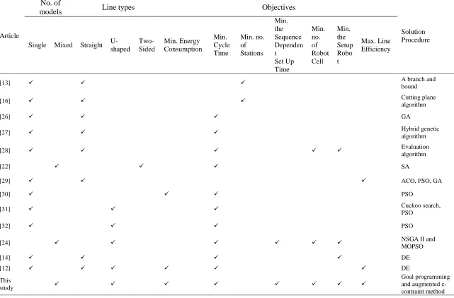
Table 1. Comparison table of the literature on the robotic assembly line balancing problem.

Article

No. of

models Line types Objectives

Solution Procedure Single Mixed Straight

U-shaped Two-Sided

Min. Energy Consumption

Min. Cycle Time

Min. no. of Stations

Min. the Sequence Dependen t

Set Up Time

Min. no. of Robot Cell

Min. the Setup Robo t

Max. Line Efficiency

[13]    A branch and

bound

[16]    Cutting plane

algorithm

[26]    GA

[27]    Hybrid genetic

algorithm

[28]      Evaluation

algorithm

[22]    SA

[29]    ACO, PSO, GA

[30]    PSO

[31]    Cuckoo search,

PSO

[32]    PSO

[24]       NSGA II and

MOPSO

[14]     DE

[12]       DE

This

study        

(8)

Rabbaniet al. / Int. J. Res. Ind. Eng 8(1) (2019) 1-xx 8

Eq. (1) is to minimize the cycle time; Eq. (2) is to minimize the robot setup and sequence dependent setup cost of the task; Eq. (3) is to minimize robot purchasing cost; Eq. (4) is to minimize energy consumption; Eq. (5) calculates the energy consumption of each workstation consists of each stations operation energy consumption and standby energy consumption, and the considered constraints are as blow:

∑ ∑(𝑃𝑇𝑖𝑚𝑟+ 𝑆𝑒𝑇𝑖𝑟+ 𝑆𝑑𝑇𝑖) ∗ (𝑋𝑖𝑗𝑚𝑟+ 𝑋𝑖𝑗𝑟) 𝑅

𝑟=1 𝐼

𝑖=1

≤ 𝐶𝑇𝑚 , ∀𝑗 ∈ 𝐽, 𝑚 ∈ 𝑀 (6)

∑ ∑ 𝑗 ∗ 𝑋ℎ𝑔𝑚𝑟 𝑅 𝑟=1 𝐽 𝑔=1 − ∑ ∑ 𝑗 ∗ 𝑋𝑖𝑗𝑚𝑟 𝑅 𝑟=1 𝐽 𝑗=1

≤ 0 , ∀ℎ ∈ 𝑝𝑟𝑡(𝑖), 𝑚_{∈ 𝑀} (7)

∑ 𝑌𝑗𝑟 𝑅

𝑟=1

≥ 2 , ∀𝑗 ∈ 𝐽 (8)

∑ ∑ 𝑋𝑖𝑗𝑚𝑟≥ 2 𝑅

𝑟=1 𝐽

𝑗=1

, ∀𝑖 ∈ 𝐼, 𝑚 ∈ 𝑀 (9)

∑ 𝐿𝑅𝑟 𝑅

𝑟=1

∗ 𝑌𝑗𝑟 ≤ 𝐿𝑊𝑗 , ∀𝑗 ∈ 𝐽 (10)

∑ 𝑊𝑅𝑟

𝑅

𝑟=1

∗ 𝑌𝑗𝑟 ≤ 𝑊𝑊𝑗 , ∀𝑗 ∈ 𝐽 (11)

∑ ∑ 𝑌𝑗𝑟 𝑅 𝑟=1 ≥ 1 𝐽 𝑗=1 (12)

𝑋𝑖𝑗𝑚𝑟∈{0,1}

, 𝑖 = 1, 2, … , 𝐼; 𝑗 = 1, 2, … , 𝐽

𝑚 = 1, 2, … , 𝑀; 𝑟 = 1, 2, … , 𝑅

(13)

𝑋𝑖𝑗𝑟∈{0,1}

, 𝑖 = 1, 2, … , 𝐼; 𝑗 = 1, 2, … , 𝐽

𝑟 = 1, 2, … , 𝑅 (14)

𝑌𝑗𝑟 ∈{0,1} , 𝑗 = 1, 2, … , 𝐽; 𝑟_{= 1, 2, … , 𝑅} (15)

(9)

2.2 Failure Rate Constraint for Each Robot

In real time, by increasing in robots’ processing time there would be a decreasing going in robot performances. Hence, we have considered a constraint, which limits the accepted failure ratio in each selected robot. The [36] has introduced the model as follows:

Where 𝜆_𝑟 indicates the initial failure in robot 𝑟; 𝑡_𝑟 represents the processing time of each robot if purchase robot 𝑟 and assigne job 𝑖 in station 𝑗 from product 𝑚 to it.

3. Multi-Objective Mathematical Programming

In Multi-Objective Mathematical Programming (MMP), more than one objective exist to optimize and there is no single optimal solution to optimize all objectives. In these cases, finding the “most preferred” solution that would cover most of the objectives and optimize them is the solution. A multiple objective can be given in the following form [37]:

𝑀𝑖𝑛 𝐹(𝑥) = [𝑓1(𝑥), 𝑓2(𝑥), … , 𝑓𝑚(𝑥)]

𝑆. 𝑡.

𝑥 ∈ 𝑋 ⊂ 𝐼𝑅𝑛

(17)

In this article, two different methods are used to find the most preferred solution: Goal Programming method and Augmented 𝜀-Constraint method.

3.1 The Goal Programming Method

The Goal Programming (GP) is an important technique to solve Multi-Objective Decision-Making (MODM) problems in finding a set of most preferred solutions. It was first presented by [37] and later on developed by other researchers [38-41]. The main purpose of GP is to minimize the deviations between the optimal solution of each objective and their aspiration levels. It can be expressed as given model:

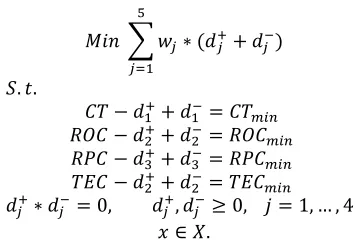
𝑀𝑖𝑛 ∑ 𝑤𝑗∗ (𝑑𝑗++ 𝑑𝑗−) 𝑚

𝑗=1

𝑆. 𝑡. 𝑓𝑗(𝑥) − 𝑑𝑗++ 𝑑𝑗−= 𝑔𝑗, 𝑗 = 1, … , 𝑚

𝑑𝑗+∗ 𝑑𝑗−= 0, 𝑑𝑗+, 𝑑𝑗−≥ 0, 𝑗 = 1, … , 𝑚

𝑥 ∈ 𝑋.

(18)

Where 𝑔_𝑗 indicates the goal for objective function 𝑓_𝑗; 𝑑_𝑗+ and 𝑑_𝑗− represent the deviation variables

under and over achievement of the 𝑗th goal. Based on Section 0, this article model in programming model is as given:

𝐹𝑅(𝑡)𝑟= 1 − 𝑒−λ𝑟𝑡𝑟

𝑆. 𝑡.

𝑡𝑟= ∑ ∑ ∑ (𝑃𝑇𝑖𝑚𝑟) ∗ (𝑋𝑖𝑗𝑚𝑟+ 𝑋𝑖𝑗𝑟) ∗ 𝑌𝑗𝑟 𝑀

𝑚=1 𝐽

𝑗=1 𝐼

𝑖=1

(10)

𝑀𝑖𝑛 ∑ 𝑤𝑗∗ (𝑑𝑗++ 𝑑𝑗−) 5

𝑗=1

𝑆. 𝑡.

𝐶𝑇 − 𝑑1++ 𝑑1−= 𝐶𝑇𝑚𝑖𝑛

𝑅𝑂𝐶 − 𝑑2++ 𝑑2−= 𝑅𝑂𝐶𝑚𝑖𝑛

𝑅𝑃𝐶 − 𝑑3++ 𝑑3−= 𝑅𝑃𝐶𝑚𝑖𝑛

𝑇𝐸𝐶 − 𝑑2++ 𝑑2−= 𝑇𝐸𝐶𝑚𝑖𝑛

𝑑𝑗+∗ 𝑑𝑗−= 0, 𝑑𝑗+, 𝑑𝑗−≥ 0, 𝑗 = 1, … , 4

𝑥 ∈ 𝑋.

(19)

3.2 The Augmented 𝜺-Constraint Method

The augmented 𝜀-constraint method is a developed version of 𝜀-constraint method and has it's own advantages. In this method, for all 𝑝 − 1 objective functions except the main one, payoff table is calculated leading to better results. To calculate the payoff table, the maximum and minimum solutions for each objective function would be calculated. Next, the range of each function is given and due to the given range, the augmented 𝜀-constraint program is calculated as follows:

𝑀𝑖𝑛 𝑓1(𝑥) − 𝛿 ∗ (𝑆_𝑟2

2+

𝑆₃

𝑟₃+ ⋯ +

𝑆_𝑝

𝑟_𝑝)

𝑆. 𝑡.

𝑓2+ 𝑆2= 𝜀2

𝑓3+ 𝑆3= 𝜀3

…

𝑓𝑝+ 𝑆𝑝= 𝜀𝑝

𝑟𝑝= 𝑓𝑝𝑚𝑎𝑥− 𝑓𝑝𝑚𝑖𝑛 , 𝑗 = 2, … , 𝑝

𝜀𝑝= 𝑓𝑝𝑚𝑎𝑥−

𝑟𝑝

𝑝∗ 𝑗, 𝑗 = 2, … , 𝑝 .

(20)

Where 𝛿 is a small number and usually between 10−3 and 10−6; 𝜀_𝑝 is the decision makers accepted tolerance in 𝑝th objective function; and 𝑗 is total objective function interval grids points. As the presented model, therefore, the article problem in this model is as follows:

Min 𝐶𝑇 − δ ∗ (S2

r₂+

S3

r₃+

S4

r₄)

𝑆. 𝑡.

𝑅𝑂𝐶+ 𝑆2= 𝜀2

𝑅𝑃𝐶 + 𝑆3= 𝜀3

𝑇𝐸𝐶 + 𝑆4= 𝜀4

𝑟𝑝= 𝑓𝑝𝑚𝑎𝑥− 𝑓𝑝𝑚𝑖𝑛 , 𝑝 = 2, 3, 4

𝜀𝑝= 𝑓𝑝𝑚𝑎𝑥−

𝑟𝑝

𝑝 ∗ 𝑗, 𝑝, 𝑗 = 2, 3, 4 .

(11)

4. Illustrative Example and Results Analysis

4.1 Test Problems

This section presents a case study of illustrated model. Consider a manufacture which has 8 kind of robots (𝑟 = 8) that can be purchased, producing 2 kinds of products (𝑚 = 2) and need to be assigned to 2 available workstations (𝑗 = 2) where exists 8 assembly tasks (𝑖 = 8) with respect to precedence processes that should be assigned to the available workstations and purchase robots. The following table represents the payoff table of objectives:

Table 2. Payoff table of the objectives.

𝐶𝑇 (𝑆𝑒𝑐) 𝑅𝑂𝐶 ($) 𝑅𝑃𝐶 ($) 𝑇𝐸𝐶 (𝐾𝑊)

1714 20000 1400000 208000 1718 8000 1400000 210660 1717 20000 1400000 207960 1722 30000 2000000 106260

In the following, we have used goal programming and augmented ε-constraint method to find the Pareto optimal solutions for each method and the results are given in following tables:

Table 3. Goal programming method optimal Pareto solutions.

Solution Number 𝐶𝑇 𝑅𝑂𝐶 𝑅𝑃𝐶 𝑇𝐸𝐶

1 1715 8000 1410000 106260

2 1717 20000 2000000 106380

3 1718.9659 22703.1 2000000 106260

4 1720 23000 2000000 106350

(12)

Table 4. Augmented ε-constraint method optimal Pareto solutions.

Solution Number 𝐶𝑇 𝑅𝑂𝐶 𝑅𝑃𝐶 𝑇𝐸𝐶

1 1714 20000 1400000 208000

2 1714 20000 1450000 199575

3 1715 18000 1400000 210640

4 1715 18000 1500000 185240

5 1715 19000 1400000 209480

6 1716 14000 1400000 209640

7 1716 17000 1450000 200175

8 1717 12000 1450000 203480

9 1717 12000 1500000 187145

10 1717 13000 1400000 210400

11 1718 8000 1400000 210660

12 1718 8000 1500000 185580

13 1718 10000 1450000 202755

14 1718 11000 1400000 210500

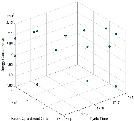
Figure 3. Operational optimal solutions of ε-augmented constraint.

(13)

4.2 Comparison Metrics

In order to compare the efficiency of augmented ε-constraint method and goal programming method, the various performance metrics are reported and we have used generational number of Pareto solutions (N), distance (GD), spacing (S), and spread (Δ) in our work and explained briefly as follows:

Generational distance: to find a solution of Q belongs to the set of P or not, the Generational

Distance (GD) evaluates an average distance of the solutions of Q from P, as follows:

The parameter 𝑑_𝑖is the Euclidean distance (in the objective space) between the solution 𝑖 ∈ 𝑄 and the nearest member of 𝑃∗:

𝑑𝑖= min

𝑘∈|𝑃∗|√ ∑ (𝑓𝑚

(𝑖)_{− 𝑓}

𝑚∗(𝑖))2

𝑀

𝑚=1

. (23)

Where 𝑓_𝑚∗(𝑖) is the m_thobjective function of the K_thmember of 𝑃∗. Intuitively, an algorithm

hasing a small value of GD is better.

Spacing. The spacing metric (𝑆𝑝) [42] is calculated with a relative distance measure between

consecutive solutions in the obtained non-dominated set as follows:

𝑆𝑝= √

1

|𝑄|∑(𝑑𝑖− 𝑑̅)2 |𝑄|

𝑖=1

. (24)

Where 𝑑𝑖 = min_{𝑘⊆𝑄∧𝑘≠𝑖}{∑𝑀𝑚=1|𝑓𝑚(𝑖)− 𝑓𝑚(𝑘)|} and 𝑑̅ is the mean value of the above distance

measure 𝑑̅ = ∑|𝑄|_𝑖=1𝑑𝑖⁄_|𝑄|. The above metric measures the standard deviations of different 𝑑_𝑖

values. When the solutions are nearly spaced, the corresponding distance measure will be small. Thus, an algorithm finding a set of non-dominated solutions has the smaller spacing (S) is better.

Spread. The spread metric (Δ) [43] measures the extent of spread achieved among the obtained solutions. Then, the following metric is to calculate the non-uniformity in the distribution:

GD =(∑ di

p |Q|

i=1 )1/p

(14)

Δ =∑Mm=1dme + ∑ |di− d̅| |Q|

i=1 ∑Mm=1dme + |Q|d̅

. (25)

Where 𝑑_𝑖 is Euclidean distance between neighboring solutions that having the mean value 𝑑̅. The parameter 𝑑𝑚𝑒 is the distance between the extreme solutions of 𝑃∗ and 𝑄 corresponding to mth

objective function. An algorithm finding a smaller value of Δ is able to find a better diverse set of non-dominated solutions.

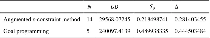
Table 5. Comparison of algorithms with respect to illustrative example.

𝑁 𝐺𝐷 𝑆𝑝 Δ

Augmented ε-constraint method 14 29568.07245 0.218498741 0.281403455 Goal programming 5 240097.4139 0.489938335 0.444503484

5. Conclusion

Most of the companies that have U-shaped robotic mixed assembly line generally come across with URMALB-II in practice. Although there are many studies about assembly line balancing problems, the papers on URMALB-II are very few. Our model tries to determine the optimal or near optimal configurations with respect to considered objectives as minimizing the cycle time, robot purchasing costs, robot operational costs, and energy consumption. In this paper, we used two different multi-objective algorithms to solve the presented model. The first algorithm was weighted goal programming and the second algorithm was augmented ε-constraint method. To solve the problem, we coded the methods in GAMS. In continue, the performance of algorithms had compared with each other. As shown in Table 5, the augmented ε-constraint produced more number of Pareto points than GP. In Generational Distance (GD), GP had a better solution but in other parameters (spacing and spread), better solutions come from augmented ε-constraint. There are several interesting points for future work, developing meta-heuristic algorithms to solve the problem and considering the real life situations such as zoning constrain and proposing a dynamic model base on the online data.

References

Groover, M. P. (1980). Automation, production systems, and computer-aided manufacturing (Vol. 1). Englewood Cliffs, NJ: Prentice-Hall.

Salveson, M. E. (1955). The assembly line balancing problem. The journal of industrial engineering, 6(3), 18-25.

(15)

Falkenauer, E., & Delchambre, A. (1992, May). A genetic algorithm for bin packing and line balancing. Proceedings of the 1992 IEEE international conference on robotics and automation (pp. 1186-1192). Nice, France, France: IEEE.

Ajenblit, D. A., & Wainwright, R. L. (1998, May). Applying genetic algorithms to the U-shaped assembly line balancing problem. Proceedings of the 1998 IEEE international conference on evolutionary computation. IEEE world congress on computational intelligence (Cat. No. 98TH8360) (pp. 96-101). Anchorage, AK, USA, USA: IEEE.

Miltenburg, G. J., & Wijngaard, J. (1994). The U-line line balancing problem. Management science, 40(10), 1378-1388.

Urban, T. L. (1998). Note. Optimal balancing of U-shaped assembly lines. Management science, 44(5), 738-741.

Scholl, A., & Klein, R. (1999). ULINO: Optimally balancing U-shaped JIT assembly lines. International journal of production research, 37(4), 721-736.

Özcan, U., Kellegöz, T., & Toklu, B. (2011). A genetic algorithm for the stochastic mixed-model U-line balancing and sequencing problem. International journal of production research, 49(6), 1605-1626.

Jonnalagedda, V., & Dabade, B. (2014). Application of simple genetic algorithm to U-shaped assembly line balancing problem of type II. IFAC proceedings volumes, 47(3), 6168-6173.

Alavidoost, M. H., Tarimoradi, M., & Zarandi, M. F. (2015). Fuzzy adaptive genetic algorithm for multi-objective assembly line balancing problems. Applied soft computing, 34, 655-677.

Nilakantan, J. M., Ponnambalam, S. G., & Nielsen, P. (2018). Energy-Efficient straight robotic assembly line using metaheuristic algorithms. Soft computing: theories and applications (pp. 803-814). Singapore: Springer.

Rubinovitz, J., Bukchin, J., & Lenz, E. (1993). RALB–A heuristic algorithm for design and balancing of robotic assembly lines. CIRP annals, 42(1), 497-500.

Nilakantan, J. M., Nielsen, I., Ponnambalam, S. G., & Venkataramanaiah, S. (2017). Differential evolution algorithm for solving RALB problem using cost-and time-based models. The international journal of advanced manufacturing technology, 89(1-4), 311-332.

Rubinovitz, J., & Levitin, G. (1995). Genetic algorithm for assembly line balancing. International

journal of production economics, 41(1-3), 343-354.

Kim, H., & Park, S. (1995). A strong cutting plane algorithm for the robotic assembly line balancing problem. International journal of production research, 33(8), 2311-2323.

Delice, Y., Aydoğan, E. K., Özcan, U., & İlkay, M. S. (2017). A modified particle swarm optimization algorithm to mixed-model two-sided assembly line balancing. Journal of intelligent manufacturing, 28(1), 23-36.

Faccio, M., Gamberi, M., & Bortolini, M. (2016). Hierarchical approach for paced mixed-model assembly line balancing and sequencing with jolly operators. International journal of production research, 54(3), 761-777.

Kara, Y., Ozcan, U., & Peker, A. (2007). An approach for balancing and sequencing mixed-model JIT U-lines. The international journal of advanced manufacturing technology, 32(11-12), 1218-1231.

Kucukkoc, I., & Zhang, D. Z. (2014). Simultaneous balancing and sequencing of mixed-model parallel two-sided assembly lines. International journal of production research, 52(12), 3665-3687. Simaria, A. S., & Vilarinho, P. M. (2009). 2-ANTBAL: An ant colony optimization algorithm for

balancing two-sided assembly lines. Computers & industrial engineering, 56(2), 489-506.

(16)

Rabbani, M., Mousavi, Z., & Farrokhi-Asl, H. (2016). Multi-objective metaheuristics for solving a type II robotic mixed-model assembly line balancing problem. Journal of industrial and production engineering, 33(7), 472-484.

Çil, Z. A., Mete, S., & Ağpak, K. (2017). Analysis of the type II robotic mixed-model assembly line balancing problem. Engineering optimization, 49(6), 990-1009.

Levitin, G., Rubinovitz, J., & Shnits, B. (2006). A genetic algorithm for robotic assembly line balancing. European journal of operational research, 168(3), 811-825.

Gao, J., Sun, L., Wang, L., & Gen, M. (2009). An efficient approach for type II robotic assembly line balancing problems. Computers & industrial engineering, 56(3), 1065-1080.

Yoosefelahi, A., Aminnayeri, M., Mosadegh, H., & Ardakani, H. D. (2012). Type II robotic assembly line balancing problem: an evolution strategies algorithm for a multi-objective model. Journal of manufacturing systems, 31(2), 139-151.

Daoud, S., Chehade, H., Yalaoui, F., & Amodeo, L. (2014). Solving a robotic assembly line balancing problem using efficient hybrid methods. Journal of heuristics, 20(3), 235-259.

Nilakantan, J. M., Huang, G. Q., & Ponnambalam, S. G. (2015). An investigation on minimizing cycle time and total energy consumption in robotic assembly line systems. Journal of cleaner production, 90, 311-325.

Nilakantan, J. M., Ponnambalam, S. G., & Huang, G. Q. (2015). Minimizing energy consumption in a U-shaped robotic assembly line. 2015 international conference on advanced mechatronic systems (ICAMechS) (pp. 119-124). IEEE.

Nilakantan, M. J., Ponnambalam, S. G., & Jawahar, N. (2016). Design of energy efficient RAL system using evolutionary algorithms. Engineering computations, 33(2), 580-602.

Manavizadeh, N., Hosseini, N. S., Rabbani, M., & Jolai, F. (2013). A Simulated Annealing algorithm for a mixed model assembly U-line balancing type-I problem considering human efficiency and Just-In-Time approach. Computers & industrial engineering, 64(2), 669-685.

Mukund Nilakantan, J., & Ponnambalam, S. G. (2016). Robotic U-shaped assembly line balancing using particle swarm optimization. Engineering optimization, 48(2), 231-252.

Li, Z., Tang, Q., & Zhang, L. (2016). Minimizing energy consumption and cycle time in two-sided robotic assembly line systems using restarted simulated annealing algorithm. Journal of cleaner production, 135, 508-522.

Chan, J. K., & Shaw, L. (1993). Modeling repairable systems with failure rates that depend on age and maintenance. IEEE transactions on reliability, 42(4), 566-571.

Charnes, A., & Cooper, W. W. (1957). Management models and industrial applications of linear programming. Management science, 4(1), 38-91.

Ignizio, J. P. (1985). Introduction to linear goal programming. Sage Publications.

Lee, S. M. (1972). Goal programming for decision analysis (pp. 252-260). Philadelphia: Auerbach

Publishers.

Li, H. L. (1996). An efficient method for solving linear goal programming problems. Journal of optimization theory and applications, 90(2), 465-469.

Pal, B. B., Moitra, B. N., & Maulik, U. (2003). A goal programming procedure for fuzzy multiobjective linear fractional programming problem. Fuzzy sets and systems, 139(2), 395-405.

Schott, J. R. (1995). Fault tolerant design using single and multicriteria genetic algorithm

optimization (Master’s Thesis, Boston, MA: Department of Aeronautics and Astronautics, Massachusetts Institute of Technology).

Kalyanmoy, D. (2001). Multi objective optimization using evolutionary algorithms (pp. 124-124).

John Wiley and Sons.