R E S E A R C H
Open Access
HyGen: generating random graphs with
hyperbolic communities
Saskia Metzler
1*and Pauli Miettinen
2*Correspondence:
[email protected] 1Max-Planck-Institute for Informatics, Saarland Informatics Campus, 66123, Saarbrücken, Germany
Full list of author information is available at the end of the article
Abstract
Random graph generators are necessary tools for many network science applications. For example, the evaluation of graph analysis algorithms requires methods for generating realistic synthetic graphs. Typically random graph generators are generating graphs that satisfy certain global criteria, such as degree distribution or diameter. If the generated graph is to be used to evaluate community detection and mining algorithms, however, the generator must produce realistic community structure, as well. Recent research has shown that a clique is not necessarily a realistic community structure, necessitating the development of new graph generators. We propose HYGEN, a random graph generator that leverages the recent research on non-clique-like communities to produce realistic random graphs with hyperbolic community structure, degree distribution, and clustering coefficient. Our generator can also be used to accurately model time-evolving communities.
Keywords: Random graph generators, Community detection, Hyperbolic community structure
Introduction
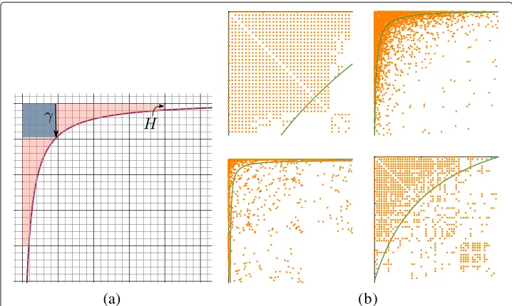
Modular structure is a characteristic of real-world networks. Its constituents, or com-munities, typically display specific patterns of connectivity. Especially in social networks, communities show a pronounced core-tail structure: a small fraction of the members have strong ties to each other and form the core. The majority of members only have ties to the core and not to each other (Laumann and Pappi1976; Alba and Moore1978; Morgan et al.1997; Reed and Selbee2001; Panzarasa et al.2009; Metzler et al.2019). This kind of intra-community structure is well described by ahyperbolic model(Araujo et al.2014; Metzler et al.2016). The hyperbolic model can express the particular core-tail structure which is frequently observed in real-world networks. It also encompasses power law-like connectivity and is suitably general to represent clique-like as well as star-like patterns of connectivity (see Fig.1b).
Understanding network organization is a primary goal of social sciences. Reaching this goal requires not only adequate models, but also suitable community detection algo-rithms. The quality of community detection algorithms is best tested on real-world data. This, however, requires significant amounts of testing data with reliable labels. Man-ual labelling is qMan-ualitatively the most adequate. In contrast, any automated community labelling procedure implies a comparison of the community detection algorithm under test to another procedure of detecting the communities. A favourable alternative to obtain
(a)
(b)
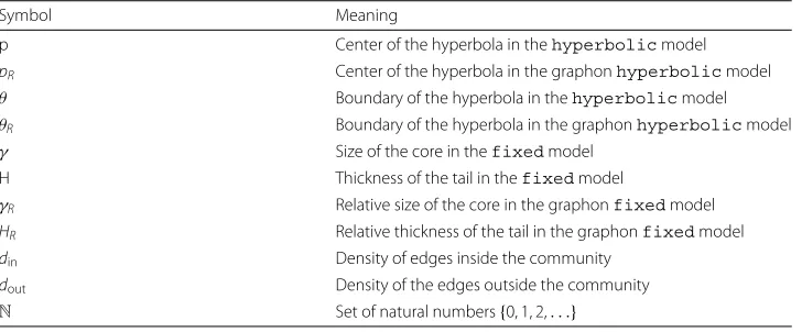
Fig. 1Visualization of parameters for the hyperbolic model, and real-world examples. Models are shown on the degree-ordered adjacency matrix of each community. Customarily, the positive domain of the coordinate system is plotted from top left. Orange dots represent edges. The solid line visualizes the hyperbolic model.aγandHbExamples of hyperbolic communities from (Metzler et al.2016)
large amounts of reliably labelled testing data is to use random graph generators that create graphs with similar properties as real-world templates.
Most random graph generators aim at modelling global properties of the graphs, such as degree distribution, clustering coefficient, or effective diameter. Hence, models such as Erd˝os and Rényi (1959), Albert and Barabási (2002), or the Forest fire model (Leskovec et al. 2005) do not generate community structure and are not applicable to commu-nity detection. Similarly, graph expansion(Park and Kim 2018; Zhang and Tay2016) andhyperbolic geometry(Krioukov et al.2010) models focus on the global modelling of real-world graphs. Kronecker graphs (Leskovec et al.2010) can be interpreted to have a community structure, but due to the recursive structure, the constructed communities have symmetries in size and shape not observed in real-world graphs.
The R-MAT generator (Chakrabarti et al.2004) is another popular model for generating random graphs with community structure. It is based on recursively subdividing the adjacency matrix into four equally sized partitions and distributing the edges within the partitions according to partition-specific probabilities. This approach allows it to mimic the degree distributions of real-world graphs, but restricts the shape of the constructed communities.
A third popular model for testing community detection algorithms is the Lancichinetti– Fortunato–Radicchi (LFR) benchmark (Lancichinetti et al. 2008), which extends the Girvan–Newman benchmark (Girvan and Newman2002). Unlike SBM or R-MAT, LFR can produce overlapping community structures and weighted and directed graphs. Com-pared to Girvan–Newman, LFR emphasizes the heterogeneous distributions of node degrees and community size. Yet, LFR generates near-uniform intra-community degree distributions, violating the assumption of non-clique-like community structures.
Orman et al. (2013) examine variations of LFR which achieve more realism with respect to transitivity and degree correlation in the generated graphs by choosing alternate ran-dom models for the initial step of the algorithm. In recent work, Fagnan et al. (2018) propose a generalization of LFR which follows the evolution patterns and characteris-tics of real networks. Unlike the present work, these works concentrate on overlapping communities.
To the best of our knowledge, however, no existing random graph generator is designed to model graphs consisting of hyperbolic communities. As many real-world graphs seem to follow a hyperbolic or core–tail model, we introduce a novel random graph genera-tor to fill this gap. HYGENgenerates modular networks with realistic intra-community structures using parameter distributions derived from observations on real graphs.
Contributions
This article extends our previous work on HYGEN (Metzler and Miettinen2019). We present the model in more detail and have improved the exposition and analysis thereof. Our novel contributions in this work are the following:
• We present an alternative formulation of the HYGENmodel as a graphon.
• We show that the graphon model is particularly suitable for modelling time-evolving communities.
• We show empirically that existing random graph generators are not suitable for generating hyperbolic community structure.
The HYGENModel
The hyperbolic community model
The hyperbolic community model of Metzler et al. (2016) generates undirected graphs. LetG = (V,E) be an undirected graph with|V| = nand|E| = m. Assume that the vertices are assigned a unique number from{0,. . .,n−1}in an arbitrary manner. We use pair(u,v)to denote both a pair of vertices and the (potential) undirected edge between them.
AcommunityofGis a tuple(VC,πC,C)whereVC ⊆ V are the nodes of the com-munity withnC = |VC|,πC:VC → {0,. . .,nC −1}is a permutation of the nodes that maps the nodes of a community to a set of indices {0,. . .,nC − 1}, and C is a set of parameters that defines the shapeof the community. We assume that the permuta-tionπCorders the nodes in descending order according to their intra-community degree degC(v)= |{u∈VC :(v,u)∈E}|.
The key feature of the hyperbolic community model is that not all edges between nodes inVCare necessarily part of the communityVC. Which edges are part of the community is defined using a functionf: {0,. . .,nC−1} × {0,. . .,nC−1} ×C → {0, 1}, themodel of the community. The functionf takes a pair of permuted node indices and the set of parameters for the community, and decides whether the edge between the nodes is part of the community. An edge(u,v)is a part of the communityCif
1 u∈VCandv∈VC; and 2 f(πC(u),πC(v),C)=1.
In what follows we will mostly omit writing the permutation. Instead, when it is clear from the context, we will denote vertices by their indices in the permutation; for instance, v,u, andwcould be denoted byi,j, andh, with the meaning thati = πC(v),j= πC(u), andh=πC(w).
Metzler et al. (2016) study three different models, calledhyperbolic,fixed, and
mixture. Despite being seemingly different, the three models are equivalent (Metzler et al.2016), and we will use them interchangeably. For the sake of completeness, we will present two of them,hyperbolicandfixed, here, as they are the two models we will need the most. Thehyperbolicmodel takes two parameters,pandθ, and the model functionfhyperbolicis
fhyperbolic(i,j,p,θ)=[(i+p)(j+p)≤θ] , (1)
where we used the Iverson bracket notation: [P]=1 if propositionPis true and [P]=0 otherwise. Thehyperbolicmodel makes the hyperbola shape of the community obvi-ous, but otherwise the parameters are not straight forward to interpret. Thefixedmodel has more interpretable parameters:γ defines the size of thecoreof the community andH indicates how thick thetailis. A core of the community is a subcommunity of people that are known by (almost) everybody else in the community, while the tail consists of the rest of the members in the community (see Fig.1a)1.
Metzler et al. (2016) show that we can transform the parameters offixedto the param-eters ofhyperbolicusing the following equations (Metzler et al. (2016), Eqs. (7) and (8)):
1The terms core and periphery are also used for similar structures (Borgatti and Everett1999). We use the notion of core
p= γ 2−(n
C−1)H
(nC−1)+H−2γ
(2)
θ = (γ−H)2(γ−nC−1)2
(nC−1+H−2γ )2
. (3)
Single community
The model for a single community is straight forward and we express it via thefixed
model. Assume, for now, that the size of the community,nC, is given. To define the com-munity infixed, we need to have the two parameters,γ andH. In our model, we assume that the relativeγ,γR = γ /nC, follows the normal distribution with some meanμand varianceσ2. Assuming we have sampled someγ =nCγR, we will sampleHby assuming thatH/γ ∼Exponential(λ)(we will motivate these distributions later using experiments with real-world data sets).
After we have sampledγ andH, we can generate a perfect communityC using the
fixedγ,H model. The communityCwill have no noise, that is, no edges between the nodes in the tail of the community and no missing edges within the community. As this is an unrealistic assumption, we will apply uniform noise to remove edges from the com-munity and add edges between tail nodes. For this, we will need two more parameters,din anddout, that describe thedensitiesof the community and of the area outside the com-munity; a fraction of 1−dinedges within the community are removed and a fraction of doutedges outside the community (i.e. between tail nodes) is added.
Multiple communities
To generate multiple communities, we use an approach similar to SBMs, and gener-ate individual communities independently of each other. For each community, we will draw the sizenCfrom distributionDsize. Our experiments suggest using the generalized extreme value distribution as the distribution of the sizes, but the power law distribution, as used by Lancichinetti et al. (2008), is a viable alternative.
After the community size is sampled, we can sampleγ andHas explained above. Do note that the way we sample them is independent of the community size, and hence we can use the same distributions for every community.
After we have sampled a noise-free community, we will remove some of its edges to obtain the desired “inside” densitydinand plant the community to the graph. The planting happens so that the communities do not overlap, similar to SBMs, but we can permute the order of the nodes, so that the hyperbolic shape is not immediately obvious. After all communities have been planted, we apply the “outside” noise to achieve thedoutdensity among the edges that are between nodes in different communities and between nodes that in the tail of the same community. The full process is detailed in Algorithm 1.
Notice that this model assumes that the “inside” noise is the same in all communities, and the “outside” noise is uniform throughout the graph (though these two types of noise can be very different, and in general,din dout). We also assume the size and shape of the communities to be uncorrelated.
Time complexity
Algorithm 1:HYGENalgorithm
Data: distributionsDsize,Dγ,DH, densitiesdin,dout, number of communitiesk
Result: random graphG
for i=1 :kdo
draw sizesfromDsize,γ fromDγ, andHfromDH scaleγ according tos, andHaccording toγ make modelfixed(γ,H)
select edges to discard uniformly at random to reachdin plant result intoG
apply noisedoutto the outside community area ofG
returnG
edges in a graph consisting only perfect communities. LetEnbe the set of edges noise addsto the graph (inter- and intra-community). Drawing the parameters and adjusting them is a constant-time operation, creating the model takesO(nC)time, and sampling the edges to discard from the community can be done in timeO|EpC|(Knuth1981, p. 137). Assuming we have kcommunities, the total time to generate a graph with no noise is Ok1+nc+ |EpC|
= O(k+ |V| + |Ep|). To add noise, we need to do sampling with-out replacement over a population ofO|V|2− |Ep|
edges, taking essentially linear time. When|Ep|and|En|are small compared to|V|2(i.e. the graph is sparse), we can sample with replacement to obtain practically the same result, takingO(|En|)time. In total, the full running time of Algorithm 1 isO(k+ |V| + |Ep| + |En|), which is only slightly more thanO(|V| + |E|).
HYGENas a Graphon
A graphon (Orbanz and Roy 2015) is a measurable functiong: [ 0, 1]×[ 0, 1]→[ 0, 1]. Graphongcan be seen as a model for random graphs: to sample a graphGfrom graphon g, one first samplesnvertices by samplingnpoints from the unit interval [ 0, 1] uniformly at random (that is,V ⊂[ 0, 1]). One then samples the edges so thatGhas edge(u,v)with probabilityg(u,v). For undirectedG,ghas to be symmetric, that is,g(u,v)=g(v,u), and the undirected edge betweenuandvis sampled as the directed edge(u,v).
The HYGEN model for one community is easy to express as a graphon. The graphon is parameterised with four parameters,pR,θR,din, anddout. The parameterspRandθR define the hyperbola as with the standard model: given two nodesu,v ∈[ 0, 1], the edge between them is part of the community (i.e.uandvare in the intra-community area of the community) if
(u+pR)(v+pR)≤θR. (4)
Parameters din and dout are as with the standard model, that is, they define the (expected) inside density and (expected) outside density. The graphon for the HYGEN model for one community is
h=
din if(u+pR)(v+pR)≤θR dout otherwise.
(5)
fixedmodel. In the standardfixedmodel, the parameterγ indicates the size of the core; in the graphon version, it indicates therelative sizeof the core, that is, which frac-tionof the nodes belongs to the core. Similarly, theHparameter in the graphon model corresponds to therelative thicknessof the tail. We denote these parameters asγRandHR, respectively. They can be derived from the hyperbola analogously to the standard case (see Metzler et al. (2016)): we can setγRas the valueu where(u +pR)(u +pR)=θRand HRas the value where(u +pR)(1+pR)=θR. This gives
γR= −pR±
θR (6)
HR= −
p2R+pR−θR pR+1
(7)
As we require thatγR,HR ∈[ 0, 1], ifpR ≥ 0, say, then (7) implies that it must be that
θR≥pR(pR+1)and then (6) takes fromγR= −pR+√θR. Similar conditions can be easily derived forpR<0 (see Metzler et al. (2016) for the conditions in the standard model).
Vice versa, we can also solvepRandθRfromγRandHR(cf. Eqs. (2) and (3)):
pR= γ 2 R−HR
−2γR+HR+1
ifγR=1 andHR=1 (8)
θR= (γR−
1)2(γR−HR)2
(−2γR+HR+1)2
ifγR=1 andHR=1. (9)
WhenγR=HR=1, we can set, for instance,pR=0 andθR=1.
Using graphons in the HYGENalgorithm is straight forward: we generate a graphon for each community based on its parameters and replace the community generation inside the for-loop of Algorithm 1 with sampling the community from its graphon, as explained above. In addition, the graphon model is particularly useful for modelling time-evolving communities. Unlike the standard HYGENalgorithm, the graphon model makes it easy to adjust the size of the community while retaining some vertices: this can be done by simply randomly discarding some of the previously-selected nodes and potentially sampling new ones. Generating a full time-evolving graph would then amount to running Algorithm1 for every time step, but instead of generating the communities from the scratch, we adjust their sizes based on the graphon model.
Unlike the standard HYGEN model, the graphon model has somewhat more random-ness. The parameterγR, for example, does not define the actual size of the core, but the expected size of the core. The actual size of the core is a binomially distributed random variable with parametersγR ands, wheresis the size of the community. Similarly, the density parametersdinanddoutare only expectations.
HYGENgraphs with specific community structures
In the above, we described HYGEN model using randomly sampled shape parameters. Normally, we would fit the hyperparameters of the distributions to some real-world data sets to obtain a realistic model for the random graphs, but in some cases, we might want to obtain specific community structures.
the third model presented by Metzler et al. (2016), themixturemodel. That model has again two parameters,x∈[−1, 1] and∈R, and the functionf defining the shape is
fmixture(i,j,x,)=(1− |x|)(i·j)+x(i+j)≤. (10)
The mixturemodel is, again, equivalent to thefixedandhyperbolic models (Metzler et al.2016). By settingx=0, it becomes clear that the model reduces to a power law; the exponent of the power law is absorbed by the parameter, as setting =1/−α (assuming >0) yields to
(ij)−α≤ .
Hence we can sample power law communities by just sampling one parameter, ∈ (0,∞).
A clique-like community is even more restricted than power law community, as we can setγ = H = nC to obtain a clique. With such fixed settings, our model reduces to a variation of SBM.
Theoretical results on HYGENrandom graphs
The HYGEN model is designed to preserve important graph properties. In addition to the hyperbolic community structure, HYGENalso preserves the degree distribution and the clustering coefficient of the graph. These two properties measure the connectivity of networks (Aggarwal and Wang2010), and are often studied with social networks. In this section, we present theoretical analysis of the HYGENrandom graphs, proving that they preserve the degree distribution and clustering coefficients (up to noise).
In the last part of this section, we discuss how the hyperbolic community structure determines the degree correlation. This measure is studied to assess to what extent nodes of similar degree connect to each other.
Degree distribution
The degree distribution is perhaps the most important global property of the graph and has been one of the main topics in many seminal papers (e.g. Watts and Strogatz (1998); Faloutsos et al. (1999); Albert and Barabási (2002)), and preserving the distribution (at least approximately) is one of the standard aims of random graph generators.
As the HYGEN graphs have disjoint communities, we will first analyse a single com-munity. For the sake of simplicity, we will study thecomplementary cumulative degree distributionF¯: {0,. . .,|V|} →[ 0, 1], whereF¯(k)is the fraction of vertices with degreeat least k. Clearly, the cumulative degree distributionF isF(k) = 1− ¯F(k). For a single community with no noise we have the following lemma.
Lemma 1 Let C=(VC,EC)be a community that follows thehyperbolic(p,θ)model perfectly. The complementary cumulative degree distributionF¯Cof C is determined by the parameters p andθ.
ProofAccording to the model, an edge(i,j)is inECif and only if(i+p)(j+p)≤θ(recall that the model assumes that the vertices are sorted by degree). Re-writing, we obtain that (i,j)∈ECif
That is, vertexihas degree at leastjif (11) holds, and conversely, ¯
FC(j)=max{i∈N:j≤θ/(i+p)−p}/|VC|.
Lemma1uses thehyperbolicmodel for the simplicity of the proof. Thanks to the the equivalence relations (2) and (3) (see also Metzler et al. (2016)), we can also state the lemma using the potentially more intuitivefixedmodel and its parameters:
Corollary 1The complementary cumulative degree distribution of C,F¯Cis determined by the parameters H andγ.
Lemma1shows that the degree distribution of a single community is determined by the model; to extend that to the full graph, it is enough to notice that as the communities are disjoint, the total degree distribution is the sum of the individual communities’ degree distributions.
Lemma 2Given a graph G = (V,E) that is a product of theHYGEN model with no
noise, its complementary cumulative degree distributionF is completely determined by the¯ parameters of its communities.
ProofLetGconsist ofkcommunitiesC1=
VC1,EC1
,. . .,Ck=
VCk,ECk
and denote bynCi= |VCi|the number of nodes in communityi. As the communities are disjoint, and there are no vertices outside the communities,
n= |V| = k
i=1 nCi.
That there is no noise means that (1) communities are perfect in the sense of Lemma1, and (2) there are no inter-community edges. Hence, by Lemma1,F¯Ci is defined by the parameters of communityCi, and
¯ F(j)= 1
n k
i=1
nCiF¯Ci(j), (12)
that is, the number of nodes inGwith degree at mostjis the sum of the numbers of nodes with degrees at mostjover all the communities.
Lemmata 1 and 2 cover the case where there is no noise. Such an assumption is usually too strict for real-world graphs, and would yield to bad modelling of real-world phenomena. When we add the noise, the model parameters (e.g.pandθ) will not be enough to define the overall edge distribution. We can show, however, that the noise has most effect to the tails of the degree distribution.
Lemma 3Let G be aHYGENgraph with no noise and G the same graph with a fraction
of q∈[ 0, 1]noise applied, that is, dout= q and din =1−q in G. The expected degree of vertex v in G,EG[d(v)], is
EG [d(v)]=d(v)+q(n−2d(v)), (13)
ProofA fraction of q edges connected tovwill be removed due to the noise, and a fraction ofqedges not connected tovwill be added. Hence,
EG[d(v)]=d(v)−qd(v)+q
n−d(v),
which simplifies to (13).
Equation13already hints that ifd(v) is large or small, the expected degree can have bigger relative changes. Letα(v)=d(v)/n, that isα(v)is therelative degreeofv. Then we can write (13) as
EG[α(v)]=EG[d(v)]/n=α(i)+q
1−2α(i), (14)
showing that the noise has the most effect on nodes withα(v) ≈ 0 orα(v) ≈ 1; on the contrary, ifα(v)=1/2, the presence of noise will have no effect on the expected degree.
The above result means that communities that have many vertices with either very few or very many neighbors are most affected by the noise. An extreme example of such a community would be a star, and similarly, communities with steep power-law curves in degree distribution would also see significant changes from small amounts of noise.
Clustering coefficient
In addition to the degree distribution, theclustering coefficientis often used to measure the connectivity of the graphs, and high clustering coefficients are associated with “small-world graphs” (Watts and Strogatz1998).
There exists two different versions of the clustering coefficient, the global clustering coefficientand thelocal clustering coefficient(Aggarwal and Wang2010).
Definition 1Given a graph G, its global clustering coefficient cc(G)is defined as
cc(G)= number of closed triplets in G
number of all triplets in G . (15)
Definition 2Given an undirected graph G = (V,E)and its vertex v ∈ V , the local
clustering coefficient ccv(G)of v in G is defined as
ccv(G)=
2|(u,w):u,w∈(v),{u,w} ∈E|
d(v)(d(v)−1) , (16)
where(v)is the neighbourhood of v.
We can again show that, up to the effects of the noise, the clustering coefficients – both local and global – are fully determined by the model parameters. We start by analysing the local clustering coefficient in a single community, as that is the most straight forward to do.
Lemma 4Let C =(VC,EC)be a community that follows thehyperbolic(p,θ) with-out any noise and let i be an arbitrary vertex of C. The local clustering coefficient cci(C)of i in C is determined entirely by p andθ.
(i)=h∈VC :h≤θ/(i+p)−p
and the set of edgesECas
EC =
i,j∈VC:j≤θ/(i+p)−p
,
showing that they both depend only onpandθ. That the degree of vertexi,d(i), depends only onpandθ follows from Lemma1.
To analyse the global clustering coefficient cc, we will first make some definitions. Define the indicator functionχ(i,j)as
χ(i,j)=
1 j≤θ/(i+p)−p
0 otherwise . (17)
This function indicates for every pair of vertices i andj if there would be an edge between them in a community following thehyperbolic(p,θ)model with no noise.
The number of closed triplets in a community following noise-freehyperbolic(p,θ) model can be counted by testing whether all of the edges between the vertices exist. DefineTcl:N3→ {0, 1}as
Tcl(i,j,h)=χ(i,j)·χ(i,h)·χ(j,h). (18)
An open triplet (wedge) is a set of three vertices connected by exactly two edges. Define To:N3→ {0, 1}as
To(i,j,h)=χ(i,j)·χ(i,h)·(1−χ(j,h)) (19)
to test whether(i,j,h)is an open triplet centred ati.
Lemma 5Let C be as in Lemma4. The global clustering coefficient cc(C)of C is entirely determined by p andθ.
ProofAs the value ofχi,jis defined bypandθ (with fixediandj), so are the values of TclandTo. We can write (15) with them as
cc(C)= i,j,h∈VCT cl(i,j,h)
i,j,h∈VC
Tcl(i,j,h)+To(i,j,h),
where we always assume thati,j, andhare disjoint.
The above Lemmata4and5can be extended to a full graph following noise-free HYGEN model.
Lemma 6Let G=(V,E)be a graph that follows theHYGENmodel with no noise. The global clustering coefficient cc(G)and the local clustering coefficient ccv(G)for any v∈V are determined through the parameters of the hyperbolic communities of G.
Table 1List of symbols
Symbol Meaning
p Center of the hyperbola in thehyperbolicmodel
pR Center of the hyperbola in the graphonhyperbolicmodel
θ Boundary of the hyperbola in thehyperbolicmodel
θR Boundary of the hyperbola in the graphonhyperbolicmodel
γ Size of the core in thefixedmodel
H Thickness of the tail in thefixedmodel
γR Relative size of the core in the graphonfixedmodel
HR Relative thickness of the tail in the graphonfixedmodel
din Density of edges inside the community
dout Density of the edges outside the community
N Set of natural numbers{0, 1, 2,. . .}
χ(u,v)=
1 ifu,v∈Cfor some communityCandπC(u)≤θC/(πC(v)+pC)−pC 0 otherwise,
where pC andθC are the parameters of the communityC andπC is the permutation associated with it. With this definition of χ, the functionsTcl and To will also work throughout the full graph, concluding the proof.
Lemma6also shows that theaverage local clustering coefficientis determined by the community parameters.
Corollary 2Let G be as above. The average local clustering coefficient cc(G) =
1
|V| v∈Vccv(G)is entirely determined by the community parameters.
It is not trivial to analyse the effects of noise to the clustering coefficient. Triangles or wedges from the inside-community area disappear, and new ones get introduced involving the outside-community area. Given the overall density of a graph, the expected number of triangles or wedges is derivable, but integrating the specific intra-community structure into this expectation remains an open problem.
Degree correlation
The degree correlation measures whether the number of links between nodes with high degree and nodes with low degree is systematically different from what is expected in a random network. A network is called assortative if nodes of similar degree tend to link to each other, and dissassortative if the network exhibits a preference for links between nodes of dissimilar degree. Both trends of correlation may occur in real world networks. While social networks tend to be assortative, other kinds of networks, including those of question-answering portals, are typically observed to be disassortative (Aggarwal and Wang2010).
Using results of prior work, we may claim that hyperbolic communities are usually dis-assortative: Jonhson et al. (2013) study the relation between nestedness of networks and disassortivity. They show that with high probability, disassortative networks are nested and vice versa. LetG = (V,E)be an undirected graph. We say Gisnested if we can order the verticesv ∈ Vin a sequence(v1,v2,. . .,vn)such thatN(vi+1) ⊆ N(vi)for all i=1,. . .,n−1. As discussed by Karaev et al. (2018), hyperbolic communities are a spe-cial case of nested matrices. Notice that also communities whose adjacency is described by a power law function are therefore disassortative since the power law is special case of the hyperbolic model.
Experimental evaluation
In this section we present the results of our empirical evaluation. We will first explain the data sets, then study how the parameters are distributed in real-world graphs, and then we study how the other random graph generators work at modelling the kind of communities observed in real-world graphs. We will then study the quality of the graphs constructed using the HYGENmodel: first, we will study how well the generated graphs fit to the model and then we will study how random the generated graphs are. Finally, we will study how good the graphon model is at modelling time-evolving communities.
We base our evaluation on the HYGENparameters. Up to noise, clustering coefficient as well as degree distribution are derivable from the HYGENparameters, as we have estab-lished in the previous section. We do not test inter-community connections such as path length, modularity, or degree correlation, since these would measure only added noise, or in case of the degree correlation of individual communities, be already predetermined through the structures we allow.
Datasets
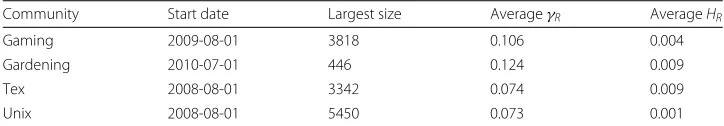
We use two different collections of real-world data sets. The first collection, calledSNAP, consists of four networks with community information from the Stanford Large Network Dataset collection (Leskovec and Krevl2014):Amazon,DBLP,Friendster, andYouTube. These are real-world social networks with ground-truth communities labeled in the data. The properties of the graphs are summarised in Table2.
Our second collection of real-world datasets is called SE and it contains four time-evolving communities from the https://stackexchange.com family of online question–answer sites (Q&A sites) (Stack Exchange 2016). The communities are https://gaming.stackexchange.com, https://gardening.stackexchange.com, https://tex. stackexchange.comandhttps://unix.stackexchange.com. The data are from Metzler et al. (2019). Some basic properties of these communities are listed in Table3. The data sets
Table 2Summary of the networks in the SNAP collection
Network Nodes Edges Communities
All 100–1000
Amazon 334 863 925 872 75 149 1 380
DBLP 317 080 1 049 866 13 477 805
Friendster 65 608 366 1 806 067 135 957 154 19 763
Table 3Basic properties of four SE communities
Community Start date Largest size AverageγR AverageHR
Gaming 2009-08-01 3818 0.106 0.004
Gardening 2010-07-01 446 0.124 0.009
Tex 2008-08-01 3342 0.074 0.009
Unix 2008-08-01 5450 0.073 0.001
The averageγRand averageHRare computed using a weighted average with the community size at each month being the
weight. The parametersγandHfor these communities are by Metzler et al. (2019)
contain a snapshot of the community at the begin of each month from the start date until November 2016.
Distributions for the parameters
Above, we suggested distributions to use for the distributions of the shape parametersγ andHand the sizenC. Here we detail how these suggestions were obtained.
For these experiments, we use theSNAPcollection of real-world data sets. We sam-ple 500 communities of size between 100 and 1000 nodes2and compute the hyperbolic models for each community to obtain empirical distributions forγ,H, and the (truncated) community sizenC.
For each of the empirical distributions for γ, H, and nC, we fit different distribu-tions (namely, generalized extreme value distribution, inverse Gaussian distribution, Birnbaum–Saunders distribution, exponential distribution, normal distribution, log-logistic distribution, gamma distribution, Rayleigh distribution, Weibull distribution, Nakagami distribution, Rician distribution, normal distribution, logistic distribution, extreme value distribution, andt-location-scale distribution). Not every distribution is applicable for each of the parameters. While the observedγs look normally distributed, Hand the community size show an exponential behaviour.
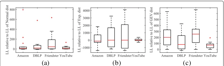
In order to validate our subjective observations, we tested how well the different dis-tributions fit using the negative log-likelihood (LL). Alternative reasonable measures for evaluation would be Akaike or Bayesian information criterion. We observe highly sim-ilar results with either of the measures and therefore only present the evaluation with respect to LL. To show the results in a concise manner, we present here only compar-isons of our chosen distributions against all other options. Namely, for every distribution Dthat is not the one we chose to model parameterp, we compute our test statistics Tp(D) = LLp(D)−LLp(D∗), whereLLp(D) is the negative log-likelihood of modelling parameterpusing distributionDandLLp(D∗)is that for the selected distribution D∗. The larger valuesTp(D)obtains, the better the selected distribution performs compared to distributionD,Tp(D)=0 indicates thatDandD∗perform equally well, and negative values indicate thatDperforms better than the chosen distributionD∗.
Based on our experiments, we propose to modelγ (relative to the community size) using the normal distribution,H(relative toγ) using the exponential distribution, and the community sizenCusing the generalized extreme value distribution. Our comparison of these distributions against others in theSNAPdatasets are presented in Fig.2.
As can be seen in Fig.2a, the normal distribution is constantly at least as good as the other distributions (i.e. there are no negative values), implying that the use of normal
(a)
(b)
(c)
Fig. 2Relative log-likelihoods (LL) of the hypothesised distributions compared to the other distributions. For each dataset, the boxplot indicates how well each parameter follows the hypothesised distribution compared to other potential distributions. Positive values indicate that the preferred distribution performs better than the others and zero indicates even performance.aγbHcsize
distribution is a valid choice. The situation when modelling the distribution of theH parameter (w.r.t.γ) is more complicated. Our experiments showed the exponential distri-bution to have the best fit, but as can be seen in Fig.2b, in some cases other distributions would be better. More experiments would be needed to give a conclusive answer to the question which distribution explains observedHs best.
For modelling the distribution of the community size (Fig.2c), the GEV distribution is always the best, and shows the strongest performance against the other distributions. Please note, however, that in this test we model the distribution of the sizes of the com-munities in a single network at one point of time; when studying the sizes of a single community over time, very different distributions might be needed (cf. Fig.8).
Limits of the current graph generators
While many of the existing random graph generators cannot be used to model commu-nity structures in networks at all, there are a number of related approaches that allow for generated graphs with community structure. To the best of our knowledge however, there exists no approach of preserving the intra-community connection patterns in the modeling process.
In this section, we detail why SBM, LFR, and R-MAT do not provide solutions to the modeling task we aim to solve. For this purpose, we compare the outcome of these generators when fitted to idealized hyperbolic communities. One may argue that such communities are not realistic and therefore not a fair basis of comparison for these generators that are designed to model real-world graphs, which are usually sparse and exhibit a certain level of noise. However, the purpose of this experiment is to see to what extent thepurehyperbolic structure can be captured at all by the different generators.
Experimental Setup. We generate single hyperbolic communities with the extremes of
(a)
(b)
(c)
(d)
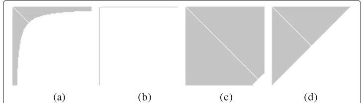
Fig. 3Adjacency matrices of idealised hyperbolic communities. The different extremes of hyperbolic structures, range from star-like to near-clique.a20%-corebstarcnear-cliquedtriangle
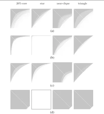
randomness. Figure5summarizes the resulting hyperbolic models that best fit the com-munities generated by the respective method. We overlay the 50 obtained models in light grey. Ideally, we would expect to see the exactly the structures of Fig.3again.
Notice that the LFR implementation strictly requires multiple communities to be gen-erated. Therefore, we provide graphs containing twice the same community as input (like illustrated in Fig.6a for the 20%-core) and use the better matching one in the evaluation of the fit quality.
SBM. The standard SBM is based on the assumption that vertices within a block are stochastically equivalent. The hyperbolic model fulfils this assumption only in the extreme case of a quasi-clique, where the size of the core equals the size of the commu-nity. The typical core-tail structure of hyperbolic communities cannot be captured (see Fig.4a). As the generated graphs after fitting the SBM model are almost uniformly dense, the hyperbolic models fitted on these outputs exhibit a huge degree of variance and often differ a lot from the original input (see Fig.5a). The high negative LL scores of the fits (see Table4) indicate that the fitted hyperbolic models are also not particularly good at explaining SBM-generated communities. Regarding the case of a near-clique, it is worth pointing out that a perfect clique would be recovered well by the SBM. The case of the near-clique (Fig.5a, column 3) is substantially harder: almost all nodes are connected to each other but a few miss some connections. For the SBM however, the primary aim is to match the overall density evenly. Thus the fit is such that many nodes are fully connected and some are connected to almost every other node, which yields into a substantially different looking hyperbolic model.
(a)
(b)
(c)
(d)
(a)
(b)
(c)
(d)
Fig. 5Hyperbolic model fitted on results of alternate generators. Each subfigure summarizes 50 repetitions of using the alternative generator to fit the respective input displayed in Fig.3. For every sample, the adjacency matrix of the closest hyperbolic model is displayed in light grey. Shades of grey result from overlaying all samples and yield a visual summarization of the observed shapes. The ideal result would be complete resemblance to the respective input.aHyperbolic model fitted on results of SBM.bHyperbolic model fitted on results of DC-SBM.cHyperbolic model fitted on results of R-MAT.dHyperbolic model fitted on results of LFR
Table 4Average best log-likelihood for 50 trials of generating hyperbolic communities with SBM, DC-SBM, R-MAT, and LFR, with standard deviations
20%-core star near-clique triangle
SBM -2354(1919) -451(1406) -282(1007) -3393(39)
DC-SBM -1545(1734) -212(713) -3238(521) -2679(768)
R-MAT -2008(38619) -440(958) -214(548) -2727(230133)
LFR -2515(7697) — -1299(17346) -3714(6250)
DC-SBM. DC-SBMs allow for variation of the degree within a community (see Fig.4b). Fitting back a hyperbolic model on the DC-SBM outcome of modelling a 20%-core struc-ture, a star, or a triangle are fairly accurate in the sense that the parameters γ and H are close to the original (see Fig. 5b). Yet, the hyperbolic models fitted on the DC-SBM-generated communities leave some amount of noise to be explained otherwise (see Table4). The DC-SBM expects a power-law degree distribution within the communities and draws edges from that one to recover the connectivity pattern inside the community. In particular the near-clique case (see Fig.5b, column 3) seems to be hard to explain by a power law. The hyperbolic model is more general in the sense that it includes power-law distributions as a special case. It also has a substantially different noise model, assuming uniform density for the inside-community area and as well as for the outside.
R-MAT. R-MAT is designed to model the degree distribution of the input data using
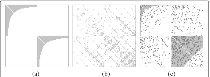
a recursive procedure. The results we observe for the single artificial communities are comparable to those of the DC-SBM (see Fig.5c). The recursive construction procedure however introduces particular structures in the data. To construct a graph, R-MAT subdi-vides the adjacency matrix recursively into quarters of certain density. This makes it hard to capture multiple communities, especially of unequal sizes. An additional experiment reveals that, already if R-MAT is fitted on a graph of two equally sized (hyperbolic) com-munities with no inter-connections, the resulting model is not capturing the this structure well (see Fig.6): by its definition, R-MAT models consist of four self-similar blocks. This means, the blocks with community structure are always mirrored to the off-diagonal, introducing many surplus links between the communities.
LFR. The LFR benchmark generates random graphs given power-law distributions for the node degree and the community size. Creating graphs that consist of a single commu-nity is not included as a special case in this approach. To still obtain comparable modelling results for the four sample hyperbolic communities (see Fig.3), we fit LFR on graphs con-sisting of twice each of those communities. The reported LL scores of fitting a hyperbolic model on the LFR results then refer to the better of the two obtained communities. While for the star pattern, we could not find a set of valid LFR parameters to describe this pattern with the procedure suggested by Lancichinetti et al. (2008), we observe that the remaining
(a)
(b)
(c)
hyperbolic communities are modeled very similar to each other by LFR, as the best hyper-bolic model to explain these communities is the same in each case (see Fig.5d). A closer look at the LFR-generated graphs reveals that they actually differ: the average degree per community is retained from the original communities, but the hyperbolic structure is lost.
Stability of the graph generation
We now turn our attention into analysing the HYGEN-generated graphs. In this section we will study how well the generated graphs fit to the real-world graphs; in the next section, we will study how random the generated graphs are.
We used the following procedure to test how well the generated graphs fit to the real-world data they were generated from: First, we fitted the hyperparameters of the parameter distributions to real-world networks from theSNAPcollection. Then we used these distributions in HYGEN to sample collections of random graphs. Finally, we com-puted the best hyperbolic model for each community in the generated graphs using the code of Metzler et al. (2016) and evaluated how accurately the found communities match to the original communities. Our hypothesis is that the found communities have simi-lar distributions of parameters as the original communities, indicating that the generated graphs retain the essence of the community structure of the original graphs.
In order to compare HYGEN, we also generated graphs using LFR and DC-SBM. Based on our experiments in the previous section, we know that they cannot model the hyper-bolic structure too well, but it is still possible that they can model all of the structure that is observed in real-world graphs.
In order to fit the hyperbolic model to the generated communities, we need to know what these communities are. Both HYGENand LFR return this information; the DC-SBM implementation we used (Nepusz2015), on the other hand, only uses this information internally and does not report it. In order to find the communities from graphs generated by DC-SBM, we will fit the model again to the generated graphs, and record the com-munity structure from the fitted models. We assume that DC-SBM correctly recovers communities when provided graphs generated by it.
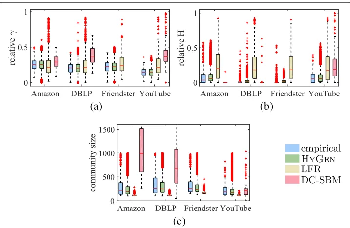
The results of this experiment, with respect toγ,H, and community size, are presented in Fig.7. It shows four boxplots for each dataset and parameter combination: the first, calledempirical, is the distribution observed from the original data, i.e. the distribution we should match, and the other three boxplots show the distributions of the parameters when fitted to the generated graphs.
In order to obtain reliable results, with HYGEN and LFR, we sampled a hundred times as many communities as was in the original data. That is, for the YouTube
data, we sampled 12900 communities, and for the other datasets, we sampled 50000 communities. DC-SBM, on the other hand, was so slow to generate the sampled graphs and fit to them that we had to limit it to one graph with 100 communi-ties for each dataset. Even with this limitation, it could not finish theFriendster data set within a week, and hence we exclude DC-SBM from the results regarding the
Friendsterdata.
(a)
(b)
(c)
Fig. 7Distributions of parameters in generated graphs compared to the empirical distributions observed in the original data.Handγare obtained after fitting hyperbolic models.aγRbHRccommunity size (data for DC-SBM>1600 not displayed)
case ofDBLPandYouTube, the first quartile ofγRin DC-SBM generated communities is above the third quartile of the original distribution, indicating a very bad fit.
Figure7b shows the results for the relativeH. Again, HYGENproduces the most accu-rate results, although the communities have a slightly thicker tail than in the original data at least inDBLPandFriendsterdata sets. On the other hand, these data sets have extremely thin tails in their communities. The communities generated by the LFR model have much thicker tails than the real communities or those generated by the HYGENmodel. In short, it is obvious that LFR cannot model the kind of thin tail real-world data sets often have. DC-SBM, on one hand, under-estimates the tail thickness for theAmazondata set, and on the other hand, over-estimates it for theYouTubedata set.
When we look at the sizes of the generated communities, in Fig.7c, we can observe that LFR has very small deviation of the community sizes, and they are generally too small, while DC-SBM generates too large communities forAmazonandDBLPdata sets, but approximately correctly-sized communities for theYouTubedata set. The communi-ties generated by HYGENhave again the best fit in the distribution of the sizes, though it seems to generate slightly less of the larger communities than what is seen in the real data. Overall, we can conclude that HYGENprovides a reasonably good fit for the original data, and significantly better than what is provided by either LFR or DC-SBM. This again shows that HYGENis the best method for modelling hyperbolic structure, and that the real-world data actually has communities with structure that cannot be captured by the other models.
Randomness of the generated graphs
be easy to obtain a very good match to the original graph by simply generating graphs that are identical copies of the original one, but these would be rather useless. Hence, it is important to study also whether the generated graphs have enough randomness.
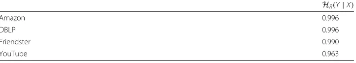
For this study, we quantify the randomness using theconditional entropyH(Y | X). Intuitively, it measures how much information is needed to describe random variableY given that we know random variableX, that is, how muchX“tells about”Y. IfY is fully determined byX,H(Y |X)=0, and ifYandXare independent,H(Y |X)=H(Y), the entropy ofY(Cover and Thomas2006). As 0≤H(Y |X)≤H(Y), we report therelative conditional entropyHR(Y |X)=H(Y|X)/H(Y)∈[ 0, 1].
We use the relative conditional entropy to compare the adjacency matrices of the dif-ferent communities (original and generated). As the graphs are undirected, we will only study the upper triangular part of the adjacency matrix. We sort the rows and columns of the adjacency matrix according to the vertex degree so that they are ordered in similar way for all graphs. We then consider the upper triangular part of the adjacency matrix as a binary vector, and identify that as a discrete random variable.
To generate the data to computeHR(Y | X), we generated 100 random graphs using HYGEN. We sampledγ andH from fitted distributions, but for the size, we used the original sizes of the communities to ensure that the random variablesXandYare of same length.
The relative conditional entropy HR(Y | X) is computed per community because communities sampled from the original graph do not maintain their context (i.e. which community overlaps with which community), and thus we cannot match the generated communities correctly to the original communities unless we generate the communities one-by-one. In addition, using the fixed sizes of communities introduces determinism not present in the full graph model that could bias the analysis.
Our results are presented in Table5. The results indicate that the information we have on the generated graphs given the original data is very small (all relative conditional entropies are larger than 0.96), that is, the generated communities are truly random. Together with the previous experiment, showing that the generation preserves the desired structure, we can conclude that HYGEN can generate random graphs that preserve the desired structure.
Modelling time-evolving communities
In this section we use the graphon version of the HYGENmodel to model time-evolving communities. Communities in social networks, especially in online Q&A sites, such as https://stackexchange.com, have surprisingly constant relative core size (Metzler et al. 2019). In other words, the relativeγ,γR, stays almost constant over time, indicating that the graphon model should be a good model for such communities. The purpose of this
Table 5Average relative conditional entropy of generated communities given the original data HR(Y|X)
Amazon 0.996
DBLP 0.996
Friendster 0.990
YouTube 0.963
experiment is to study whether that is true; in particular, whether the graphon model can generate time-evolving communities that behave similarly to the real ones.
In these experiments, we used the four communities from theSEcollection, described in Table3. Notice that here each dataset is just one community; this is sufficient for this experiment, as multi-community graphs would not change the behaviour of single com-munities. A graphon was initialised for each community using the relative parametersγR andHR from Table3 and a new community was sampled for every month in the data. We did not model the size of these communities, but used the real sizes. Similarly, we kept the same number of nodes from the previous month as was kept in the real data. Also, the sampling was done without adding any noise. This way we can concentrate on the shape of the community; the modelling of the size, or the amount of the overlap, over time is an interesting problem for future work (as Fig.8 shows, there is no com-mon trend in the sizes) and adding the noise will not change the analysis of the shape. As the tail height parameterHRis almost zero for every community (as is the case with essentially all communities like this (Metzler et al.2019)), we do not report any results on that one.
Figure8shows the results for the fourSEcommunities. The blue line shows the true γRfor each month (computed by Metzler et al. (2019)). The red line shows the average
γRcomputed from 100 samples from the graphon, and the shaded red area extends two standard deviations above and below the average (though clipping at 0).
As we can see in the blue lines, all communities have much higher values of γR at the beginning of their lives but soon the values converge to a lower value and stay rather constant. The biggest reason for the behaviour at the begin seems to be
the size of the community (depicted as black line in the figures): initially all com-munities start small, but as they grow, the relative core size γR stabilises. This can be readily seen, for instance, from the gardening community, that has a cyclic pat-tern in its size: the value ofγR varies the most when the community has the smallest sizes.
The graphon model can capture this variance based on size very well. The larger the sample (i.e. community), the smaller the standard deviation around the expected core sizeγR. Consequently, the samples follow the behaviour of the real graphs very closely, having much higher deviation at the early stages of the communities and stabilizing as the community grows. Notice that the model even follows the individual peaks very well (e.g. in unix community), even if the initial values are usually more than two standard deviations away from the average.
Overall, this experiment shows that the graphon model can be used very effectively to model time-evolving hyperbolic communities, even though there are some important future directions to explore. The current model selects the members that leave the com-munity uniformly at random; potentially more realistic model would depend, for instance, on the length of the node’s membership in the community and on its degree. Also, we did not model the community size over time. In order to generate fully synthetic graphs, this is a very important feature, although as can be seen already from Fig.8, different commu-nities can have so different behaviour that a single distribution is probably never sufficient to model all of them.
Discussion and conclusions
Being able to generate random graphs with realistic community structure is important for testing community detection algorithms and for understanding how realistic graphs behave. Recent research has shown that real-world communities have much richer struc-ture than the typically-assumed quasi-clique. Our model, HYGEN, is capable of generating random graphs with this richer structure, making them more realistic. The proposed model can also formulated as a graphon; a modelling that is particularly well-suited for modelling time-evolving graphs.
While HYGENis already an improvement over the state-of-the-art random graph gener-ators, there are still important topics of further development. The first important topic is to incorporate more realistic noise models to HYGEN. At the present, the model assumes uniform noise with different probabilities of eliminating real edges and adding spurious ones. Our experiments, however, indicate that the noise is correlated with the size of the community. Incorporating a size-dependent noise model for removing the true edges is somewhat straight forward, but modelling similar noise for inter-community edges requires future work.
The HYGEN-generated communities have currently too thick tails compared to what we see in the real world. This might be because the distribution we use to model the tail thickness parameter (Exponential) is not concentrated strongly enough, or it might have something to do with the noise model.
specifying the amount of mixture among communities. The real challenge however is not the definition of such a model, but its evaluation. Available test data from real world net-works only comes with community information with respect to the nodes. Assuming the hyperbolic model, overlap can either be within the intra-community area, or outside. In both cases, we would observe overlapping nodes, but only in the first case the communi-ties actually overlap. Due to the lack of data to evaluate the realism of generated graphs with overlapping communities, we leave this extension of the model for future work.
HYGEN has its obvious use for testing community detection algorithms. A compre-hensive comparison of community detection algorithms, as done by Orman et al. (2013) and Fagnan et al. (2018), is a planned future work. HYGENcan generate realistic graphs equipped with reliable labelling of the communities. Besides this, HYGENmight serve as an anonymization tool to study the structure of social networks without revealing the participants identities.
Abbreviations
DC-SBM: Degree-corrected stochastic block model; GEV: Generalized extreme value; LFR: Lancichinetti–Fortunato–Radicchi benchmark; LL: Log-likelihood; SBM: Stochastic block model
Acknowledgements
The authors wish to express their gratitude for Prof. Stephan Günnemann and Dr. Dóra Erd ˝os for helpful discussions during the preparation of this manuscript.
Authors’ contributions
SM designed the HyGen generator, did the theoretical analysis and implementation, and conducted the empirical experiments. PM helped with the design and analysis, designed the graphon version and did its implementation and experimental evaluation. Both authors participated equally on writing of the manuscript. Both authors read and approved the final manuscript.
Funding Not applicable.
Availability of data and materials
The datasets used and/or analysed during the current study are available from the corresponding author on reasonable request. All source code used in the current study is implemented in Matlab (tested on Matlab 2018b) and is available from the corresponding author on reasonable request.
Competing interests
The authors declare that they have no competing interests.
Author details
1Max-Planck-Institute for Informatics, Saarland Informatics Campus, 66123, Saarbrücken, Germany .2University of Eastern Finland, P.O. Box 1627, FI-70211, Kuopio, Finland .
Received: 21 March 2019 Accepted: 2 July 2019
References
Abbe E (2017) Community detection and stochastic block models: recent developments.https://arxiv.org/abs/1703. 10146. Accessed 21 Mar 2019
Aggarwal CC, Wang H (eds) (2010) Managing and Mining Graph Data. Springer, New York Alba RD, Moore G (1978) Elite social circles. Sociol Methods Res 7(2):167–188
Albert R, Barabási A-L (2002) Statistical mechanics of complex networks. Rev Mod Phys 74:47–97
Araujo M, Günnemann S, Mateos G, Faloutsos C (2014) Beyond blocks: Hyperbolic community detection. In: Calders T, Esposito F, Hüllermeier E, Meo R (eds). Proc. 2014 European Conference on Machine Learning and Principles and Practice of Knowledge Discovery from Databases (ECMLPKDD ’14). Springer, Berlin. pp 50–65
Borgatti SP, Everett MG (1999) Models of core/periphery structures. Soc Netw 21:375–395
Chakrabarti D, Zhan Y, Faloutsos C (2004) R-MAT: A Recursive Model for Graph Mining. In: Berry MW, Dayal U, Kamath C, Skillicorn DB (eds). Proc. 4th SIAM International Conference on Data Mining (SDM ’04). Society for Industrial and Applied Mathematics, Philadelphia. pp 442–446
Cover TM, Thomas JA (2006) Elements of Information Theory. Wiley, Hoboken Erd ˝os P, Rényi A (1959) On random graphs I. Publi Math Debrecen 6:290
Faloutsos M, Faloutsos P, Faloutsos C (1999) On power-law relationships of the Internet topology. In: Chapin L, Sterbenz JPG, Parulkar GM, Turner JS (eds). Proc. ACM SIGCOMM 1999 Conference on Applications, Technologies,
Architectures, and Protocols for Computer Communication (SIGCOMM ’99). ACM, New York. pp 251–262 Girvan M, Newman MEJ (2002) Community structure in social and biological networks. Proc Nat Acad Sci USA
99(12):7821–7826
Holland P, Laskey K, Leinhardt S (1983) Stochastic blockmodels: First steps. Soc Netw 5(2):109–137
Jonhson S, Domínguez-García V, Muñoz MA (2013) Factors Determining Nestedness in Complex Networks. PLoS ONE 8(9):74025
Karaev S, Metzler S, Miettinen P (2018) Logistic-Tropical Decompositions and Nested Subgraphs. In: 14th International Workshop on Mining and Learning with Graphs, London.http://www.mlgworkshop.org/2018/papers/MLG2018_ paper_35.pdf
Karrer B, Newman MEJ (2011) Stochastic blockmodels and community structure in networks. Phys Rev E 83:016107 Knuth DE (1981) The Art of Computer Programming Vol. 2: Seminumerical Algorithms. 2nd. Addison-Wesley, Reading Krioukov D, Papadopoulos F, Kitsak M, Vahdat A, Boguñá M (2010) Hyperbolic geometry of complex networks. Phys Rev E
82:036106
Lancichinetti A, Fortunato S, Radicchi F (2008) Benchmark graphs for testing community detection algorithms. Phys Rev E 78(4):046110
Laumann EO, Pappi FU (1976) Networks of Collective Action: A Perspective on Community Influence Systems. Academic Press, New York
Leskovec J, Krevl A (2014) SNAP Datasets: Stanford Large Network Dataset Collection.http://snap.stanford.edu/data. Accessed 11 Feb 2016
Leskovec J, Kleinberg J, Faloutsos C (2005) Graphs over time: Densification laws, shrinking diameters and possible explanations. In: Grossman R, Bayardo RJ, Bennett KP (eds). Proc. 11th ACM SIGKDD International Conference on Knowledge Discovery and Data Mining (KDD ’05). ACM, New York. pp 177–187
Leskovec J, Chakrabarti D, Kleinberg J, Faloutsos C, Ghahramani Z (2010) Kronecker graphs: An approach to modeling networks. J Mach Learn Res 11:985–1042
Metzler S, Günnemann S, Miettinen P (2016) Hyperbolae are no hyperbole: Modelling communities that are not cliques. In: Bonchi F, Domingo-Ferrer J, Baeza-Yates RA, Zhou Z-H, Wu X (eds). Proc. 16th IEEE International Conference on Data Mining (ICDM ’16). IEEE Computer Society, Los Alamitos. pp 330–339
Metzler S, Miettinen P (2019) Random graph generators for hyperbolic community structures. In: Aiello LM, Cherifi C, Cherifi H, Lambiotte R, Lió P, Rocha LM (eds). Proc. 7th International Conference on Complex Networks and Their Applications (COMPLEX NETWORKS ’18). Springer, Cham. pp 680–693
Metzler S, Günnemann S, Miettinen P (2019) Stability and dynamics of communities on online question-answer sites. Soc Netw 58:50–58.https://doi.org/10.1016/j.socnet.2018.12.004
Morgan DL, Neal MB, Carder P (1997) The stability of core and peripheral networks over time. Soc Netw 19(1):9–25 Nepusz T (2015) blockmodel: Fitting stochastic blockmodels to empirical networks.https://github.com/ntamas/
blockmodel. Accessed 4 Mar 2019
Orbanz P, Roy DM (2015) Bayesian models of graphs, arrays and other exchangeable random structures. IEEE Trans Patern Anal 37(2):437–461
Orman GK, Labatut V, Cherifi H (2013) Towards realistic artificial benchmark for community detection algorithms evaluation. Int J Web Based Commun 9(3):349
Panzarasa P, Opsahl T, Carley KM (2009) Patterns and dynamics of users’ behavior and interaction: Network analysis of an online community. J Am Soc Inf Sci Technol 60(5):911–932
Park H, Kim M-S (2018) EvoGraph: An Effective and Efficient Graph Upscaling Method for Preserving Graph Properties. In: Guo Y, Farooq F (eds). Proc. 24th ACM SIGKDD International Conference on Knowledge Discovery and Data Mining (KDD ’18). ACM, New York. pp 2051–2059
Reed PB, Selbee LK (2001) The Civil Core in Disproportionality in Charitable Giving, Volunteering, Civic Participation. Nonprofit Volunt Sect Q 30(4):761–780
Stack Exchange Inc (2016) Stack Exchange Data Dump.https://archive.org/details/stackexchange. Accessed 24 Jan 2017 Watts DJ, Strogatz SH (1998) Collective dynamics of ’small-world’ networks. Nature 393(6684):440–442.https://doi.org/10.
1038/30918
Zhang JW, Tay YC (2016) GSCALER: Synthetically Scaling A Given Graph. In: Pitoura E, Maabout S, Koutrika G, Marian A, Tanca L, Manolescu I, Stefanidis K (eds). Proc. 19th International Conference on Extending Database Technology (EDBT ’16). OpenProceedings.org, Konstanz. pp 53–64
Zhu Y, Yan X, Moore C (2014) Oriented and degree-generated block models: generating and inferring communities with inhomogeneous degree distributions. J Compl Netw 2(1):1–18.https://doi.org/10.1093/comnet/cnt011
Publisher’s Note