A Study of Decomposition Methods for Multilabel Classification

UNIVERSIDAD DE OVIEDO

!

MASTER IN SOFT COMPUTING

AND INTELLIGENT DATA ANALYSIS

PROYECTO FIN DE MASTER MASTER PROJECT

A STUDY OF DECOMPOSITION METHODS FOR MULTILABEL CLASSIFICATION

Bego˜na H. Men´endez L´opez July, 2012

UNIVERSIDAD DE OVIEDO

!

MASTER IN SOFT COMPUTING

AND INTELLIGENT DATA ANALYSIS

PROYECTO FIN DE MASTER MASTER PROJECT

A STUDY OF DECOMPOSITION METHODS FOR MULTILABEL CLASSIFICATION

Bego˜na H. Men´endez L´opez July, 2012

TUTOR / ADVISOR:

Dr. Juan Jos´e del Coz Velasco - Artificial Intelligence Center (AIC) Dr. ´Oscar Luaces Rodr´ıguez - Artificial Intelligence Center (AIC)

Abstract

Multilabel classification is a task commonly required in many fields nowadays. It is an extension of conventional classification in which each instance may be associated with more than one label. Some examples of applications where multilabel classification is employed are media contents, functional genomics and directed marketing.

There are different kinds of methods for multilabel classification tasks. Some of them, transform the problem while others extend specific learning algorithms in order to handle multilabel data. A particular subset of the former are decomposition methods which split multilabel classification tasks into simplier ones. This project is focused on these methods. Specifically, a study of Binary Relevance (BR) method in relation with other decomposition methods is done.

BR is a very simple and common approach that learns a binary classifier for each one of the labels of the original problem. It presents some advantages, like its linear complexity with the number of labels, but it has the disadvantage that it does not consider dependence among labels. Nevertheless, as it is shown in this work, the performance of this algorithm is not as bad as it could be thought when comparing it with others methods. Its performance is closely related to the evaluation metric and to the target loss function optimized by the base learner used.

Additionaly, also an study of some others decompostion methods (CC, DBR, NS and STA) was done in order to determine if it is better to use actual labels or predictions in the training phase and if better performance is obtained employing only previous ones in a chain structure or all of them. The conclusion is that, in general, it is better to use actual labels but it depends again on the evaluation metric applied.

Contents

1 Introduction 1

1.1 Project Objectives . . . 1

2 Multilabel Classification 3 2.1 Formal Framework for Multilabel Classification . . . 3

2.1.1 Evaluation Measures . . . 3

Example-based measures . . . 4

Label-based measures . . . 5

2.2 State of the art . . . 5

2.2.1 Problem Transformation Methods . . . 6

2.2.2 Algorithm Adaptation Methods . . . 7

2.2.3 Decomposition Methods . . . 9

Binary Relevance Method (BR) . . . 9

The Classifier Chain Model (CC) . . . 10

Stacking Algorithm for Multilabel Classification . . . 11

Nested Stacking (NS) . . . 11

Dependent Binary Relevance Models (DBR) . . . 12

2.3 Label Dependence . . . 13

2.4 Related tasks . . . 14

3 Experimentation 17 3.1 Introduction . . . 17

3.2 Experiment 1: Optimizing the Accuracy . . . 18

3.2.1 Metodology . . . 18

3.3 Experiment 2: OptimizingF1 . . . 23

3.3.1 Metodology . . . 23 3.3.2 Experimental Results . . . 24

4 Conclusions 27

4.1 Summary of contributions and results . . . 27 4.2 Future work . . . 28

List of Figures

2.1 Properties of the different methods aimed at detecting label dependence. 9 3.1 Friedman-Nemenyi Test of Experiment 1 for F1 Example-based, F1

micro and F1 macrowith a significance level of 95%. . . 22

3.2 Friedman-Nemenyi Test of Experiment 1 for Jaccard Index,

List of Tables

3.1 Properties of the datasets used in the experiments. . . 18 3.2 Results of Experiment 1 (Optimizing F1) for F1Example − based,

F1M icro and F1M acro. . . 20

3.3 Results of Experiment 1 (Optimizing F1) for Jaccard Index, Hamming

Loss and Subset 0/1 Loss. . . 21 3.4 Results of Experiment 2: Optimizing Hamming Loss. . . 25

Chapter 1

Introduction

In multilabel classification, each instance is associated with more than one label, unlike conventional classification. The aim is to obtain models that automatically assign to the objects the labels that better describe them.

Nowadays, multilabel classification methods are increasingly required by modern applications. For example, it is common that media contents (text documents, movies or songs) are tagged with several labels to briefly inform the user about their content [Monta˜n´es et al.,2011].

Other applications in which multilabel classification is required are [Tsoumakas et al., 2010]: semantic annotation of images [Zhang and Zhou, 2007a] and video, functional genomics [Blockeel et al., 2006; Elisseeff and Weston, 2005; Cesa-Bianchi et al., 2006], music characterization into emotions [Wieczorkowska et al.,2006;Li and Ogihara,2006, 2003] and directed marketing [Zhang et al.,2006].

1.1

Project Objectives

This work is a study of decomposition methods for multilabel classification. These methods are those that are based on decomposing the original problem into a collection of subproblems, one for each different label. This modus operandi produces, at least, as many binary models as the number of labels the original problem presents.

There are various decomposition methods. Differences among them lie in the way of making that decomposition, in the information used to generate the models or in the relations among those models.

The most common decomposition method is Binary Relevance (BR). It is the simplest one and makes an assumption that, in most real problems is not verified. BR assumes label independence which means that it does not consider possibly relationships among labels. Anyway, despite this issue, the performance of this method is not bad at all. It is true that, usually, new decomposition methods proposed obtain better performance than BR, but many times the comparisons made are not as fair as they should be. This

Chapter 1. Introduction

is mainly motivated because the complexity of multilabel classification and the fact that compared methods are different among them and the obtained performance depends on many factors.

More specifically, problems usually have many labels which implies that decomposition methods have to learn many models and this is much more complex than learning only a unique model as in other classification tasks occurs. Besides that, these models can be learned with different learners depending on the classification method used and, what is more, there are many different evaluation metrics that can be applied and some methods obtain good results in some measures while others obtain better performance for other different measures.

All of these issues provoke that sometimes experimental results are incomplete and it makes relatively easy finding methods that improve the performance of BR in some evaluation metrics.

The aim of this project is to discuss some of these decomposition methods and experimentally compare them in order to try to demonstrate if they are significantly better than BR and for which measures.

Chapter 2

Multilabel Classification

2.1

Formal Framework for Multilabel Classification

Let L = {`1, `2, . . . , `m} be a finite and non-empty set of labels, and let X be an

input space. We consider a multilabel classification task given by a training set S = {(x1,y1), . . . , (xn,yn)}, whose instances were independently and randomly obtained from an unknown probability distribution P(X,Y) on X × Y, in which the output spaceY is the power set ofL, in symbolsP(L). In order to make the notation easier to read, we define yi as a binary vector, yi = {y1, y2, . . . , ym}, in which each component yj = 1 indicates the presence of label `j in the set of relevant labels of xi. Using this convention, the output space can be also defined asY ={0,1}m_.

The goal of a multilabel classification is to induce a hypothesis h : X −→ Y from S, that correctly predicts the subset of labels from L for a new unlabeled instance

x. Without any loss of generality, this hypothesis can be seen as a combination of a collection of sub-hypotheses, h(x) = (h1(x), h2(x), . . . hm(x)), one per label, in which eachhj takes the form of

hj :X −→ {0,1}, (2.1.1)

and it is able to predict if the label `j must be attached to the instance x or not [Monta˜n´es et al.,2011].

2.1.1

Evaluation Measures

Several metrics have been proposed in order to measure the performance of multilabel classifiers. Tsoumakas and co-workers [Tsoumakas et al., 2010] divide them into example-based and label-based measures.

Chapter 2. Multilabel Classification

Example-based measures

These measures are calculated over all examples of the evaluation data set. They obtain the average differences of the actual and the predicted sets of labels.

In [Monta˜n´es et al.,2011], the following ones, extracted from the Information Retrieval field, are gather together:

• Jaccard indexcomputes the percentage of relevant labels predicted in the subset formed by the union of returned and relevant labels1,

J accard(y,h(x)) = Pm i=1[[yi = 1 andhi(x) = 1]] Pm i=1[[yi = 1 or hi(x) = 1]] . (2.1.2)

• Precision determines the fraction of relevant labels in the predicted labels, P recision(y,h(x)) =

Pm

i=1[[yi = 1 andhi(x) = 1]]

Pm

i=1[[hi(x) = 1]]

. (2.1.3)

• Recall is the proportion of relevant labels of the example correctly predicted, Recall(y,h(x)) = Pm i=1[[yi = 1 and hi(x) = 1]] Pm i=1[[yi = 1]] . (2.1.4)

• F1 is the evenly weighted harmonic mean of Precision and Recall,

F1(y,h(x)) = 2Pm i=1[[yi = 1 andhi(x) = 1]] Pm i=1([[yi = 1]] + [[hi(x) = 1]]) . (2.1.5)

The measures presented above let us know if relevant labels have been detected or not, because they are biased towards the methods that correctly predict relevant label. Two different evaluation metrics are:

• Hamming loss, which is defined as the proportion of labels whose relevance is incorrectly predicted: Hamming(y,h(x)) = 1 m m X i=1 [[yi 6=hi(x)]]. (2.1.6)

• Subset 0/1 loss, looks if predicted and relevant label subsets are equal or not. Zero−One(y,h(x)) = [[y6=h(x)]]. (2.1.7)

Section 2.2. State of the art

Label-based measures

Any of the previous presented measures can be used here, although in Information Retrieval tasks, the usual ones are precision, recall and F1. The difference with the

former case is that, as their name indicates, these evaluation metrics are averaged over all labels. It means that the corresponding measure is calcuted over each label separately and then the average is determined over all labels.

There are two ways for calculating the average, called macro-averaging and micro-averaging [Yang,1999]. In macro-averaging, one contingency table per label is used and then, the average is calculated over all labels, while in micro-averaging, the contingency tables of individual labels are merged into a single table whose cells are computed as the sum of the sum of the corresponding cells in the local tables. Finally, this resulting table is used to calculate the global performance.

Considering a binary evaluation measureB(tp, tn, fp, fn) [Tsoumakas et al.,2010] where tp is the number of true positives, tn the number of true negatives, fp the number of false positives and fn the number of false negatives. Let tpl, tnl, f pl and f nl the same measures for a label l. The macro-averaged and micro-averaged versions ofB are calculated as follows: • Macro-averaged measure Bmacro= 1 m m X l=1 B(tpl, f pl, tnl, f nl). (2.1.8) • Micro-averaged measure Bmicro = 1 mB( m X l=1 tpl, m X l=1 f pl, m X l=1 tnl, m X l=1 f nl). (2.1.9)

2.2

State of the art

Tsoumakas and co-workers [Tsoumakas et al., 2010; Tsoumakas and Katakis, 2007] group multilabel classification methods into those ones that transform the multilabel classification problem either into one or more single-label classification problems and those methods that extend specific learning algorithms in order to handle multilabel data directly.

The first ones are called problem transformation methods, while the second ones are algorithm adaptation methods. Below, most important algorithms of both groups are exposed. Besides that, another subsection about decomposition methods is added in this work. As it name denotes, these methods split the multilabel classification problem into others simplier problems. In fact, they could be considered part of problem transformation methods but they are treated separately because this work is centered on them.

Chapter 2. Multilabel Classification

Apart from this classification, there are other approaches, called thresholding strategies, which determine a probabilistic threshold for each instance. According to [Ram´on Quevedo et al., 2011], these strategies provide an efficient way to implement multilabel learners that somehow take into account the interdependence of labels for each instance. The overall performance of a prediction of a set of labels prevails against that of each label.

2.2.1

Problem Transformation Methods

These methods are independent of the classification algorithm. They are used to convert a multilabel task into one or more single-label tasks. Probably, the most common transformation method is Binary Relevance (BR) that is also a decomposition method and it is explained in Section 2.2.3.

There are two inmediatly possible transformations [Boutell et al., 2004]. The first one consists on subjectively or randomly select one the labels of each example and discard the rest. The second one constructs the new data set taking only the single-label examples from the multi-label data set and discarding the rest. These approaches are not very useful because they discard a lot of relevant information from the original data set.

Other simple transformations commented in [Tsoumakas et al.,2010] would be different versions of the first presented approach like select for each instance the most frequent label among all examples or the least frequent one and also another method, called copy, that consists on replacing each multilabel instance with n new examples, where n is the number of labels of the original instance, and assigning one different of the n labels to each one of the examples. A variation of the copy method, called copy-weight, associates a weight of _n1 to each one of the produced examples.

Label powerset method (LP) considers each different set of labels that exists in a multilabel data set as a single label. This is a simple but effective problem transformation method that has been used in [Boutell et al., 2004; Diplaris et al., 2005]. Given a new instance, the single-label classifier of LP outputs the most probable class, which is actually a set of labels.

One of the disadvantages of this method is that it may produce data sets with a large number of classes and few instances per class. There are other related methods that try to improve LP method dealing with these problems. One of them is the pruned problem transformation (PPT) method [Read, 2008]. It uses a small threshold defined by the user and prunes away label sets that ocurrs less times than it. Besides that, this algorithm optionally introduces disjoint subsets of the label sets existing more times than the threshold, to replace the discarded information.

Another approach based on LP method is the random k-labelsets (RAkEL) method [Tsoumakas and Vlahavas, 2007]. It constructs an ensemble of LP classifiers that are trained using a different small random subset of the set of labels. After that, a ranking of labels is produced by averaging the zero-one predictions of each model per each one

Section 2.2. State of the art

correlations into account and avoids the problem of the LP method.

In [Zhang and Zhou, 2007b], the authors propose a method that, in the first stage, transforms each example into a bag of instances, where each instance in the bag corresponds to the difference between that example and the prototype vector of a class (this prototype is calculated by averaging all instances of the training set that belong to that label). In the second stage, a two level classification strategy is employed to learn from the transformed data set.

Apart from these problem transformation methods in [Tsoumakas et al., 2010] are commented others [H¨ullermeier et al.,2008;F¨urnkranz et al.,2008] used to solve ranking problems instead of classification ones.

2.2.2

Algorithm Adaptation Methods

An extensive recopilation of these methods is done in [Tsoumakas et al., 2010; Tsoumakas and Katakis, 2007]. Below, some of them will be commented.

[Clare and King,2001] adapted the C4.5 algorithm to deal with multilabel data sets. To do this, they modified the entropy formula and allowed leaves of the tree to potentially be a set of class labels. The resultant algorithm is similar to the original one and to generate rules from the decision tree, it does it in the usual way except when it is the case that a leave is a set of classes, that a separate rule will be generated for each class. Two extensions of AdaBoost for multilabel problems have been proposed in [Schapire and Singer, 2000]. AdaBoost.MH is designed to minimize Hamming loss, while AdaBoost.MR is designed to find a hypothesis which places the correct labels at the top of the ranking.

[De Comit´e et al., 2003] proposed an algorithm that extends AdaBoost.MH and produces sets of rules that can be viewed as trees like alternating decision trees. The main advantages of this method are the production of multilabel models that can be understood by humans and the hability to handle heterogeneous input data: discrete and continous values and text data.

Back-propagation algorithm has been adapted by [Zhang and Zhou,2006] to multilabel learning. The main modification of the algorithm is the introduction of a new error function to handle multiple labels.

In [McCallum,1999], the author of the paper defines a Bayesian approach to multilabel document classification, in which, a probabilistic generative model represents the multilabel nature of a document indicating that the words in a document are produced by a mixture of words distribution, one for each topic. In a first step, the labels are selected (they are the set of classes for the document); then, a set of mixture weights for these classes are produced and, finally, each word is generating by first selecting a class according to these mixture weights and after that, letting that class generate a single word.

Given a new document, the label set that is most likely is selected with Bayes rule. This approach for the classification of a new document follows the paradigm of the Label

Chapter 2. Multilabel Classification

powerset (LP) method , where each different set of labels is considered independently as a new class.

Another similar approach for multilabel text classification is proposed in [Ueda and Saito, 2002] and a deconvolution method to estimate the individual contributions of each label to a given item is proposed in [Streich and Buhmann, 2008].

In [Ghamrawi and McCallum,2005], the authors explore multilabel conditional random field (CRF) classification models that directly parameterize label co-ocurrences in multilabel classification. Two graphical models are proposed in this sense. The first one, called collective multilabel, captures co-occurence patterns among labels, while the second one, called collective multilabels with features, tries to capture the impact that an individual feature has on the co-occurrence probability of a pair of labels.

Three enhancements of Support Vector Machine to treat multilabel data sets in text classification tasks are proposed in [Godbole and Sarawagi, 2004]. The first one is an algorithm that exploits correlation between related classes in the documents. In this approach the final classifier is formed by a conjunction of SVM and BR algorithms. It could be considered an extension of BR method and, therefore, it constitutes a decomposition method that is explained in more detail in Section 2.2.3.

The other two extensions proposed in [Godbole and Sarawagi, 2004] are designed for improving the margin of SVMs in order to obtain better multilabel classifications. In ConfMat approach, the margin is improved by removing negative training instances of a complete label if it is very similar to the positive label, based on a confusion matrix estimated using any fast and moderately accurate classifier on a held out validation set and, on the other hand, BandSVM improvement consists in removing very similar negative training instances that are within a threshold distance from the learned hyperplane.

Also some approaches [Luo and Zincir-Heywood, 2005; Wieczorkowska et al., 2006; Spyromitros et al., 2008; Zhang and Zhou, 2007a] based on the kNN (k Nearest Neighbors) classifier are proposed to treat multilabel data sets. According to [Tsoumakas et al., 2010], the first step in all these methods is the same as in kNN and what differentiates them is the aggregation of the label sets of these examples. [Thabtah et al.,2004] propose an associative classification approach, called multi-class, multi-label associative classification (MMAC) which consists of three phases: rules generation, recursive learning and classification. In the first phase, it scans the training data to discover and generate a complete class-association-rules (CAR). In the second phase, MMAC removes the examples associated with this rule set and recursively learns a new rule set from the remaining examples until no further frequent items are left. Finally, in the third phase, the rules sets derived at each iteration are merged into a single multi-label rule.

Finally, in [Veloso et al., 2007], an associative classification approach for multilabel classification is proposed. The model is induced in an instance-based fashion, in which the test instance is used as a filter to remove irrelevant features from the training data. Then, a specific model is induced for each test instance, providing a much better

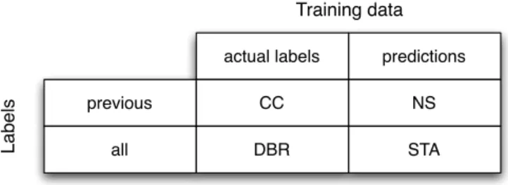
Section 2.2. State of the art predictions actual labels previous all NS CC STA DBR Training data Labels

Figure 2.1: Properties of the different methods aimed at detecting label dependence.

2.2.3

Decomposition Methods

Decomposition methods split multilabel classification tasks into others simplier tasks. In this section, decomposition methods shown in Figure 2.1 which, later, in Chapter are going to be analized experimentally, are presented. Besides them, another algorithm, called AID, is also commented here. The reason of being explained in this Section, is that it is a decomposition method similar to the other ones. Nevertheless, it is not included in the experimentation because, unlike the others decomposition methods explained, it combines models.

Apart from, formally introducing BR method, the aim of this section is to discuss the characteristics of each one of these methods and analyze the relationships among them and their differences.

All of these methods, excepting BR, are based on extending the feature space employed for generating the models of each label. In this sense, these methods can be classified according to two factors:

• the kind of information that they use to reflect dependencies among labels (actual labels or predictions from others methods).

• the dependencies that they are able to detect (among all the labels or among subsets of them).

Binary Relevance Method (BR)

This method learns m binary classifiers, one for each different label in the original data set, where each single model is learned independently of the rest, using only the information of the considered label and discarding the rest of labels. Using a formal notation, m hypotheses h1, h2, . . . , hm are induced, each of them being responsible for predicting the relevance of one label, using X as an input space:

Chapter 2. Multilabel Classification

Despite of being a very simple approach, it presents several advantages [Monta˜n´es et al., 2011]: any binary method can be taken as base learner, it has linear complexity with respect to the number of labels and it can be easily parallelized.

Besides that, as it is exposed in [Read et al., 2011], BR is theorically simple and intuitive. It is also highly resistant to overfitting label combinations because it does not expect examples to be associated with previously-observed combinations of labels as other methods, like LP, do and, since labels have a one-to-one relationship with binary models, they can be added and removed without affecting the rest of the models (this characteristic may be exploited in dinamic scenarios).

The principal disadvantage of this method is given by the fact that it ignores relationships among labels so if there are such correlations, this approach may fail to predict some label combinations. In relation to this, BR is tailored for every loss function whose risk minimizer can be expressed solely in terms of marginal distributions as, for example, Hamming loss and, on the other hand, this method will, in general, not be able to yield risk minimizing predictions for losses as subset 0/1 [Dembczy´nski et al., 2012, 2010a].

The Classifier Chain Model (CC)

This is a method proposed in [Read et al., 2009b] and extended by the same authors in [Read et al., 2011]. This algorithm is based in the BR method but it overcomes the disadvantages of BR, like not taking into account label dependences, and achieves higher predictive performance while it mantains a computational complexity of the same order as that of the Binary Relevance method.

As BR, CC involvesmbinary classifiers, one for each label, but it presents the difference with the Binary Relevance method that these classifiers are linked along a chain so they form a classifier chain.

In the training phase, the attribute space of each classifier is augmented with the actual label information of all previous labels in the chain. For instance, if the chain follows the order λ1 →λ2 →. . .→λm, then the functional form of each classifierhj will be:

hj :X × {0,1}j−1 −→ {0,1}, (2.2.2)

In this phase, all binary models can be learned in parallel because only actual label information is requiered in order to extend the feature spaces. Nevertheless, in the test phase, each classifierhjin the chain is responsible for predicting the binary association of thejthlabel given the attribute space extended by all prior binary relevance predictions in the chain, so the classifiers must be applied following the order of the chain. In symbols: h(x) = (h1(x), h2(x, h1(x)), h3(x, h1(x), h2(x, h1(x))), . . .).

In the Classifier Chain model, the order of the chain affects the accuracy. That is why [Dembczy´nski et al.,2010a] extended this algorithm proposing a probabilistic approach called Probabilistic Classifier Chains (PCC). They apply the product rule to compute

Section 2.2. State of the art P(y|x) =P(y1|x) m Y j=2 P(yj|x, y1, . . . , yj−1), (2.2.3)

The probabilities can be obtained from the classifiers of the chain when using a probabilistic learner.

PCC obtains much better results than CC because the former estimates the entire joint distribution of labels while the second one takes sequential decisions, but, on the other hand, PCC has a higher computational cost that, in practice, limits its applicability to data sets with a small number of labels.

Besides these methods, [Dembczy´nski et al., 2010a] also proposed an ensemble version of the PCC method, called EPCC and [Read et al.,2011] proposed an ensemble version of CC method, that is called ECC.

ECC is designed to avoid the influence that the order of the labels in the chain has on the performance of the CC method. ECC trainsmCC classifiers, each of them is given a random chain ordering and is trained on a random selection of the training instances sampled with replacement.

Stacking Algorithm for Multilabel Classification

[Godbole and Sarawagi, 2004] proposed an extension of the stacked generalization learning paradigm [Wolpert, 1992], usually known as stacking, for multilabel classification. It is a method for the combination of multiple classifiers on top of BR and its main advantadge is that considers the potential dependences among labels. This approach builds a stack of two groups of classifiers. Specifically, in the learning phase, the first level is formed by the same classifiers applied in the BR method. In symbols, h1_{(x) = (h}1

1(x), . . . , h1m(x)). In the second level, or meta-level, the feature space is extended including the binary outputs of all models of the first level and another group of binary models is learned: h2_(x,y0_{) = (h}2

1(x,y

0_{), . . . , h}2

m(x,y

0_{)), where} y0 =h1_(x).

The key idea is to extend the original data set with m aditional features, where m is the total number of labels of the original data set, containing the predictions of each binary classifier. Then m new binary classifiers are applied to the extended data set. In the testing phase, when classifying a new example, the procedure is the same: the binary classifiers of the first round are firstly used and their output is appended to the instance to form a meta-example that is then categorized by the classifiers of the second round. The final predictions are the outputs of the meta-levels classifiers, h2_{(x), using}

the outputs ofh1_{(x) exclusively to obtain the values of the augmented feature space.}

Nested Stacking (NS)

This method has been proposed in [Senge et al., 2012]. It arises with the idea of overcome a possible flaw of CC method: the fact that, as a result of its nature, CC

Chapter 2. Multilabel Classification

has to deal with ”noisy” test data. Specifically, in the training phase, CC uses the true values of preceding labels so the classifier is learned in ”clean” training data, but in the test phase, this information is not available and it has to be replaced by estimations coming from the corresponding classifiers, which are possibly incorrect predictions. This kind of noise may affect the performance of each classifier in the chain and, moreover, since each classifier relies on its predeccesors, a single false prediction might be propagated and even be reinforced along the whole chain.

The algorithm presented in the paper and called Nested Stacking differs from CC method in using predicted labels y₁0, . . . , y_j0₋₁ in the training phase instead of the true labelsy1, . . . , yj−1. This ensures that the data distribution is the same both in training

and in testing phases which is a key assumption in machine learning not verified by CC algorithm.

Dependent Binary Relevance Models (DBR)

Dependent Binary Relevance approach is a method proposed in [Montan´es et al.] that represents a natural extension of BR strategy for exploiting conditional label dependence. The idea for proposing this method relies on the hypothesis that object descriptions are enough to correctly predict certain situations, as BR method does in several cases, however, other cases also require to know the presence or absence of related labels for obtaining accurate predictions.

In the training phase, a group of binary classifiers is formed. It has as many classifiers as the numbers of labels and each classifier hj uses the actual labels of training data. In symbols:

h(x,y) = (h1(x, y2, . . . , ym), . . . , hm(x, y1, . . . , ym−1)), (2.2.4)

Formally, each model h2

j is defined as:

h2_j :X × {0,1}m−1 _{−→ {0,1}.}

(2.2.5) In the testing phase, the actual labels are not available. In this sense, DBR method is similar to CC approach that has also to face this issue. Despite the authors suggest that any multilabel method can be used to obtain the estimations of the actual labels, the straightforward solution is to employ BR for that purpose. Then all the methods presented in this section are comparable.

Formally, the inputs for the classifier hj will be (x, y10, . . . , y 0 i−1, y0i+1, . . . , y 0 m) where y 0 i estimations will be provided by the selected multi-label classifier.

Another algorithm, closely related to DBR is AID (Aggregating Independent and Dependent Models ) which was proposed by [Monta˜n´es et al., 2011]. It combines two typical approaches for multilabel classification: assuming label independence and

Section 2.3. Label Dependence

The idea of this method is supported on the fact that there are methods based on the first of these approaches like, BR, and others, based on the second one, that use the information about other labels in order to make their predictions. Formally, the second approach can encapsulate the former because a label-dependent model can also capture those cases that an independent model predicts correctly. However, learning reliable dependent models becomes more difficult when relationships among labels are complex; that is why the authors of the paper present a method where both approaches are used in a complementary way. In this method two groups of models are combined: the first one assumes label independence and the classifiers build are the same as in the BR method (or the first level of the stacking approach [Godbole and Sarawagi, 2004]), h1(x) = (h1₁(x), . . . , h1_m(x)). The second group of binary classifiers try to detect conditional dependences among labels, so they consider the actual information of all other labels: h2_{(x,y) = (h}2

1(x, y2, . . . , ym), . . . , hm2 (x, y1, . . . , ym−1)). That is, the

same models learned by DBR. The information about real labels can only be used in the training phase because, in the test phase, this information is unknown, so when learning a new example, the classifiers of the first group,h1_{, are applied first and then,}

their binary outputs substitute the information of the labels to form the models of the second group of classifiers h2_.

Once having calculated the two previous models, the final output of the AID method is calculated aggregating both groups of responses:

h(x) = ⊕( (h1

1(x), . . . , h 1

m(x)), (2.2.6)

(h2₁(x, h1₂(x), . . . , h1_m(x)), . . . , h2_m(x, h1₁(x), . . . , h1_m−1(x))) ),

in which ⊕ may be the or() function for multilabel classification or other function selected depending on the target loss function and on the specific learning task.

2.3

Label Dependence

According to [Monta˜n´es et al., 2011], multilabel learning presents two challenging problems: the first one is related to the computational complexity and scalability of the algorithms and the second one concerns the fact that, in multilabel classification problems, labels usually present some relationships among them. The first problem is out of the scope of this work but the second one is not, so it is commented below. Recently, many methods that try to detect and exploit dependences among labels in multilabel classification problems have been proposed. They could be classified [Monta˜n´es et al., 2011] according to: the size of the subset of labels whose dependences are searched for and depending on the type of correlations they seek to capture. On the first group, it is possible to find methods that only consider pairwise relations between labels [Elisseeff and Weston, 2005; F¨urnkranz et al., 2008; Qi et al., 2007; Schapire and Singer, 2000;Zhang and Zhou, 2006] and other ones that consider bigger subsets of labels in order to look for correlations among them [Read et al.,2008,2009a;

Chapter 2. Multilabel Classification

Tsoumakas and Vlahavas, 2007]. There are also some methods that take into account the influence of all the rest of labels when predicting each one of them [Cheng and H¨ullermeier, 2009; Godbole and Sarawagi, 2004].

On the other hand, when classifying methods according to the type of correlations they try to find, there are ones that look for conditional label dependence (dependence of the labels for a specific instance) like [Dembczy´nski et al., 2010a; Ghamrawi and McCallum, 2005; Read et al., 2009a; Tsoumakas et al., 2010] and others that seek for unconditional dependence (independent of any concrete example) like, for example, [Cheng and H¨ullermeier, 2009; Godbole and Sarawagi,2004; Zhang and Zhou, 2006]. Applying these classifications to the methods studied in this project, STA and DBR belong to the group of methods that consider the influence of all the rest of the labels to predict each one of them, while, on the other hand, CC and NS are methods that only take into account a subset of labels when predicting them. Besides that, NS and STA look for unconditional dependence whereas CC and DBR seek for conditional label dependence [Dembczynski et al., 2010].

This problem concerning relationships among labels also affects the performance of different evaluation metrics. Related to this, in [Dembczy´nski et al.,2010a], the authors analyze the connection between conditional label dependence and risk minimization for Hamming loss (Eq. 2.1.6) and subset 0/1 loss (Eq. 2.1.7). According to their results, the first one can, in principle, be minimized without taking conditional label dependence into account but it does not occur the same way for the subset 0/1 loss. Besides that, in [Dembczy´nski et al., 2010b], the authors show that minimizing the subset 0/1 loss may come along with a very high regret in terms of Hamming loss and vice versa. Refering specifically to some classification methods, as BR does not take label dependence into account, neither conditional nor unconditional, it is tailored for every loss function whose risk minimizer can be expressed solely in terms of marginal distributions as, for example, Hamming loss and, on the other hand, BR will, in general, not be able to yield risk minimizing predictions for losses as subset 0/1. On the other hand, CC performs much better with respect to 0/1 loss [Dembczy´nski et al.,2012].

2.4

Related tasks

In this section, some tasks related to multilabel classification are briefly described [Tsoumakas et al., 2010; Tsoumakas and Katakis, 2007]. They are mentioned here in order to avoid any possible confusion among them and multilabel classification caused by their similar names.

• Multilabel Ranking[Brinker et al.,2006]: Ordering a set of labels according to their relevance to a query instance, so that the topmost labels are more related with the instance.

Section 2.4. Related tasks

• Hierarchical Multilabel Classification: In hierarchical classification problems, the labels in a data set present a hirarchical structure. It means that each class is subdivided into more specific class which could also be subdivided. When instances are tagged with more than one node of the hierarchical structure, it is a hierarchical multilabel classification task.

• Multiple-label Problems [Jin and Ghahramani, 2002]: This task is not common in real world applications. It concerns the semi-supervised classification problems where each instance is associated with more than one classes, but only one of the those classes is the true class of the example.

• Multiple-instance Learning or Multi-instance Learning [Maron and Lozano-P´erez, 1998]: It is a variation of supervised learning consisting on learn a concept given positive and negative bags of instances. Specifically, labels are assigned to bags of instances where each bag may contain several instances. Only one instances is needed to be positive for a bag to be tagged as positive, but all instances are requiered to be negative in a negative bag.

• Multitask Learning [Caruana,1997]: Many similar tasks are tried to be solved in parallel usually using a shared representation and taking advance of the commom characteristics of these tasks.

Chapter 3

Experimentation

3.1

Introduction

Two experiments were performed in this work. Both experiments aim a common objetive that is to compare the performance of BR method in relation with the performance of the other methods, optimizing different measures depending on the experiment. To be more specific, in Experiment 1, base classifiers optimize the accuracy in each label, so BR is expected to optimize Hamming Loss, while in Experiment 2, F1

is optimized, therefore, the idea of this experiment is to test if BR optimizes F1macro

as it should happen. Besides that, in Experiment 1, a particular objective is aimed at comparing decomposition methods in Figure 2.1 in order to observe if it is better to use the actual labels or the predictions in the training phase and if it is preferable to employ all of them, like in STA and DBR methods, or only previous ones like in CC and NS methods.

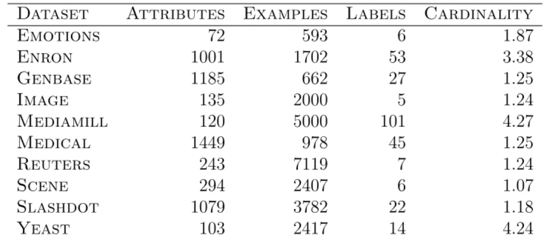
The experiments were performed over several multi-label data sets whose main properties are shown in Table 3.1. As it can be seen, they are quite different among them in the number of attributes, examples, labels and cardinality (number of labels per example). The number of attributes ranges from 72 to 1449, whereas the number of examples varies from 593 to 7119 in emotions and reuters data sets respectively. Image, emotions, reuters and scene sets have a reduce number of labels, whereas mediamill include 101 labels. Regarding the cardinality, mediamill and yeast reach the first positions (4.27 and 4.24 respectively). Emotions and enron form a group of medium cardinality (1.87 and 3.38 respectively), whereas the rest hardly reach a cardinality of 1.

Chapter 3. Experimentation

Table 3.1: Properties of the datasets used in the experiments.

Dataset Attributes Examples Labels Cardinality

Emotions 72 593 6 1.87 Enron 1001 1702 53 3.38 Genbase 1185 662 27 1.25 Image 135 2000 5 1.24 Mediamill 120 5000 101 4.27 Medical 1449 978 45 1.25 Reuters 243 7119 7 1.24 Scene 294 2407 6 1.07 Slashdot 1079 3782 22 1.18 Yeast 103 2417 14 4.24

3.2

Experiment 1: Optimizing the Accuracy

3.2.1

Metodology

In this experiment, all methods shown in Figure 2.1 were tested over all data sets in Table 3.1.

The binary base learner employed to obtain single classifiers for each label was the

logistic regression of Lin et al. [2008]. The regularization parameter C was established for each binary model performing a grid search over the values C ∈ {10p _{| p ∈} [−3, . . . ,3]} optimizing the accuracy estimated by means of a balanced 2-fold cross validation repeated 5 times. This guarantees the binary classifiers for a particular label of all methods to be exactly the same when their respective feature spaces coincide. Unlike [Read et al.,2011], no threshold selection procedure is applied in this experiment, and instead t = 0.5 is used for deciding the relevance of a label in all cases. In fact, the goal is to study the behavior of all approaches without the influence of other factors that may bias the results. Therefore, the differences between all of them are mainly due to the different feature spaces used.

The evaluation metrics applied are explained in Section 2.1.1. For those measures which are defined on a per instance basis, the value for a test set is the average over all instances. On the other hand, recall that, in F1macro, one contingency table per

label is used and then, the average is calculated over all labels, while in F1micro the

contingency tables of individual labels are merged into a single table whose cells are computed as the sum of the sum of the corresponding cells in the local tables and, finally, this resulting table is used to calculate the global performance.

The scores reported, displayed as percentages for all measures, were estimated by means of a 10-fold cross-validation. The ranks of each data sets are indicated in brackets. In case of ties, average ranks are shown. The average ranks over all data sets are computed

Section 3.2. Experiment 1: Optimizing the Accuracy

Finally, according to the recommendations exposed in [Demˇsar, 2006] for comparing several methods, a two-step statistical test procedure is carried out. The first step consists of a Friedman test of the null hypothesis that all rankers have equal performance. Then, in case that this hypothesis is rejected, a Nemenyi test to compare learners in a pairwise way is conducted. Since we are comparing 5 algorithms over 10 data sets, the critical rank differences are 2.30, 1.93 and 1.74 for significance levels of 1%, 5% and 10%, respectively.

3.2.2

Experimental Results

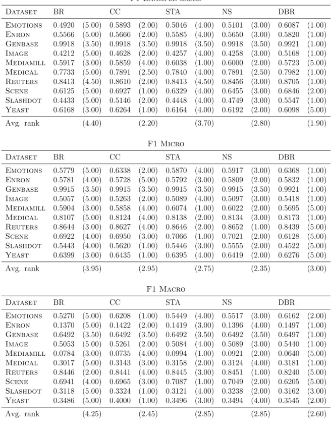
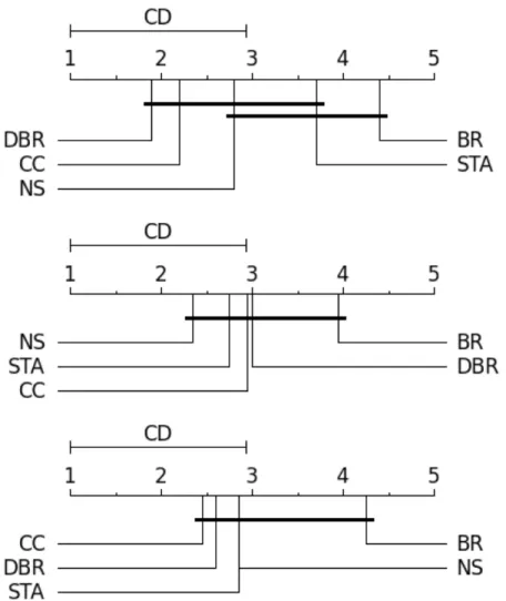
Results of Experiment 1 are shown in Table 3.2 and Table 3.3. Besides, Figure 3.1 and Figure 3.2 show the results for Nemenyi Tests done in Experiment 1 with a significance level of 95%. In these diagrams, all algorithms are compared against each other. The top line in the diagrams is an axis in which are represented the average ranks of the methods where the lowest (best) ranks are to the left. Groups of algorithms that are not significantly different (at the established significance level) are connected.

In Table 3.2 and Figure 3.1, it is possible to observe that BR is in the last position in the ranking of the algorithms according to its performance inF1example−based, F1macro

andF1micro, but inF1macroand F1microthere are no significative differences among

all the algorithms because all of them are connected in the results of the Nemenyi Test. Only inF1example−based, there is a significance difference between BR and DBR and

CC algorithms.

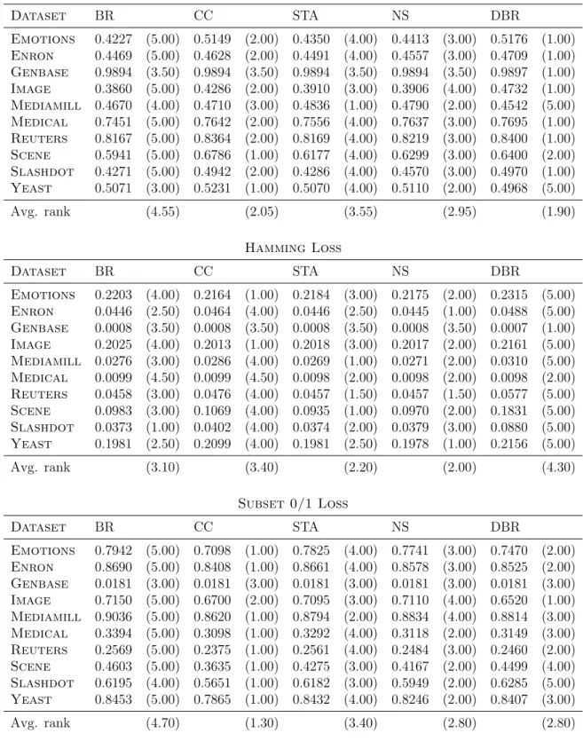
In Nemenyi Tests for Subset 0/1 and Jaccard Index, shown in Figure 3.2, BR is also in the last position in the ranking of the algorithms, but as it already occured in previous figure, this algorithm only presents significative differences with one or two algorithms (with DBR and CC in Nemenyi Test for Jaccard Index and with CC in the test for subset 0/1). The result of CC for Subset 0/1 measure verifies what was expected because, as it was commented in Section 2.3, CC optimizes this evaluation metric [Dembczy´nski et al., 2012].

Nevertheless, in the case of Nemenyi Test for Hamming Loss, it is possible to observe that BR is not significantly different to any of the others methods. It is important to highlight that, in this case, BR is situated in the ranking in a better position than CC which is an algorithm than, in the rest of measures is positioned better than BR and it occurs the same with DBR. This method is also in a worse position than BR in the results obtained for Hamming Loss. In fact, Hamming Loss is the measure in which BR obtains better results.

Therefore, these results show, as it was expected, that using base classifiers that optimize the accuracy, BR optimizes Hamming Loss and obtains a competitive performance in this measure in relation with the rest of algorithms of the experiment. On the other hand, another aim of this experiment was to analyze if better performance is obtained using actual labels (CC and DBR methods) or predictions (NS and STA) in the training phase and if it is better to use all of them (DBR and STA) or only a subset of them (previous actual labels in CC or previous predictions in NS). To answer this

Chapter 3. Experimentation

Table 3.2: Results of Experiment 1 (Optimizing F1) for F1Example−based, F1M icro

and F1M acro. F1 Example-based Dataset BR CC STA NS DBR Emotions 0.4920 (5.00) 0.5893 (2.00) 0.5046 (4.00) 0.5101 (3.00) 0.6087 (1.00) Enron 0.5566 (5.00) 0.5666 (2.00) 0.5585 (4.00) 0.5650 (3.00) 0.5820 (1.00) Genbase 0.9918 (3.50) 0.9918 (3.50) 0.9918 (3.50) 0.9918 (3.50) 0.9921 (1.00) Image 0.4212 (5.00) 0.4628 (2.00) 0.4257 (4.00) 0.4258 (3.00) 0.5168 (1.00) Mediamill 0.5917 (3.00) 0.5859 (4.00) 0.6038 (1.00) 0.6000 (2.00) 0.5723 (5.00) Medical 0.7733 (5.00) 0.7891 (2.50) 0.7840 (4.00) 0.7891 (2.50) 0.7982 (1.00) Reuters 0.8413 (4.50) 0.8610 (2.00) 0.8413 (4.50) 0.8456 (3.00) 0.8705 (1.00) Scene 0.6125 (5.00) 0.6927 (1.00) 0.6329 (4.00) 0.6455 (3.00) 0.6846 (2.00) Slashdot 0.4433 (5.00) 0.5146 (2.00) 0.4448 (4.00) 0.4749 (3.00) 0.5547 (1.00) Yeast 0.6168 (3.00) 0.6264 (1.00) 0.6164 (4.00) 0.6192 (2.00) 0.6098 (5.00) Avg. rank (4.40) (2.20) (3.70) (2.80) (1.90) F1 Micro Dataset BR CC STA NS DBR Emotions 0.5779 (5.00) 0.6338 (2.00) 0.5870 (4.00) 0.5917 (3.00) 0.6368 (1.00) Enron 0.5781 (4.00) 0.5728 (5.00) 0.5792 (3.00) 0.5809 (2.00) 0.5832 (1.00) Genbase 0.9915 (3.50) 0.9915 (3.50) 0.9915 (3.50) 0.9915 (3.50) 0.9921 (1.00) Image 0.5057 (5.00) 0.5263 (2.00) 0.5089 (4.00) 0.5097 (3.00) 0.5418 (1.00) Mediamill 0.5904 (3.00) 0.5858 (4.00) 0.6074 (1.00) 0.6022 (2.00) 0.5695 (5.00) Medical 0.8107 (5.00) 0.8124 (4.00) 0.8138 (2.00) 0.8134 (3.00) 0.8173 (1.00) Reuters 0.8644 (3.00) 0.8627 (4.00) 0.8646 (2.00) 0.8652 (1.00) 0.8439 (5.00) Scene 0.6922 (4.00) 0.6950 (3.00) 0.7066 (1.00) 0.7021 (2.00) 0.6128 (5.00) Slashdot 0.5443 (4.00) 0.5620 (1.00) 0.5446 (3.00) 0.5555 (2.00) 0.4522 (5.00) Yeast 0.6399 (3.00) 0.6435 (1.00) 0.6395 (4.00) 0.6419 (2.00) 0.6276 (5.00) Avg. rank (3.95) (2.95) (2.75) (2.35) (3.00) F1 Macro Dataset BR CC STA NS DBR Emotions 0.5270 (5.00) 0.6208 (1.00) 0.5449 (4.00) 0.5517 (3.00) 0.6162 (2.00) Enron 0.1370 (5.00) 0.1422 (2.00) 0.1419 (3.00) 0.1396 (4.00) 0.1497 (1.00) Genbase 0.6492 (3.50) 0.6492 (3.50) 0.6492 (3.50) 0.6492 (3.50) 0.6497 (1.00) Image 0.5053 (5.00) 0.5261 (2.00) 0.5084 (4.00) 0.5089 (3.00) 0.5440 (1.00) Mediamill 0.0784 (3.00) 0.0735 (4.00) 0.0994 (1.00) 0.0921 (2.00) 0.0640 (5.00) Medical 0.3017 (5.00) 0.3143 (3.00) 0.3158 (2.00) 0.3124 (4.00) 0.3181 (1.00) Reuters 0.8446 (2.00) 0.8441 (4.00) 0.8445 (3.00) 0.8451 (1.00) 0.8240 (5.00) Scene 0.6941 (4.00) 0.6965 (3.00) 0.7087 (1.00) 0.7049 (2.00) 0.6205 (5.00) Slashdot 0.3118 (5.00) 0.3324 (1.00) 0.3121 (4.00) 0.3238 (2.00) 0.3162 (3.00) Yeast 0.3486 (5.00) 0.4000 (1.00) 0.3496 (3.00) 0.3494 (4.00) 0.3545 (2.00) Avg. rank (4.25) (2.45) (2.85) (2.85) (2.60)

Section 3.2. Experiment 1: Optimizing the Accuracy

Table 3.3: Results of Experiment 1 (OptimizingF1) for Jaccard Index, Hamming Loss

and Subset 0/1 Loss.

Jaccard Index Dataset BR CC STA NS DBR Emotions 0.4227 (5.00) 0.5149 (2.00) 0.4350 (4.00) 0.4413 (3.00) 0.5176 (1.00) Enron 0.4469 (5.00) 0.4628 (2.00) 0.4491 (4.00) 0.4557 (3.00) 0.4709 (1.00) Genbase 0.9894 (3.50) 0.9894 (3.50) 0.9894 (3.50) 0.9894 (3.50) 0.9897 (1.00) Image 0.3860 (5.00) 0.4286 (2.00) 0.3910 (3.00) 0.3906 (4.00) 0.4732 (1.00) Mediamill 0.4670 (4.00) 0.4710 (3.00) 0.4836 (1.00) 0.4790 (2.00) 0.4542 (5.00) Medical 0.7451 (5.00) 0.7642 (2.00) 0.7556 (4.00) 0.7637 (3.00) 0.7695 (1.00) Reuters 0.8167 (5.00) 0.8364 (2.00) 0.8169 (4.00) 0.8219 (3.00) 0.8400 (1.00) Scene 0.5941 (5.00) 0.6786 (1.00) 0.6177 (4.00) 0.6299 (3.00) 0.6400 (2.00) Slashdot 0.4271 (5.00) 0.4942 (2.00) 0.4286 (4.00) 0.4570 (3.00) 0.4970 (1.00) Yeast 0.5071 (3.00) 0.5231 (1.00) 0.5070 (4.00) 0.5110 (2.00) 0.4968 (5.00) Avg. rank (4.55) (2.05) (3.55) (2.95) (1.90) Hamming Loss Dataset BR CC STA NS DBR Emotions 0.2203 (4.00) 0.2164 (1.00) 0.2184 (3.00) 0.2175 (2.00) 0.2315 (5.00) Enron 0.0446 (2.50) 0.0464 (4.00) 0.0446 (2.50) 0.0445 (1.00) 0.0488 (5.00) Genbase 0.0008 (3.50) 0.0008 (3.50) 0.0008 (3.50) 0.0008 (3.50) 0.0007 (1.00) Image 0.2025 (4.00) 0.2013 (1.00) 0.2018 (3.00) 0.2017 (2.00) 0.2161 (5.00) Mediamill 0.0276 (3.00) 0.0286 (4.00) 0.0269 (1.00) 0.0271 (2.00) 0.0310 (5.00) Medical 0.0099 (4.50) 0.0099 (4.50) 0.0098 (2.00) 0.0098 (2.00) 0.0098 (2.00) Reuters 0.0458 (3.00) 0.0476 (4.00) 0.0457 (1.50) 0.0457 (1.50) 0.0577 (5.00) Scene 0.0983 (3.00) 0.1069 (4.00) 0.0935 (1.00) 0.0970 (2.00) 0.1831 (5.00) Slashdot 0.0373 (1.00) 0.0402 (4.00) 0.0374 (2.00) 0.0379 (3.00) 0.0880 (5.00) Yeast 0.1981 (2.50) 0.2099 (4.00) 0.1981 (2.50) 0.1978 (1.00) 0.2156 (5.00) Avg. rank (3.10) (3.40) (2.20) (2.00) (4.30) Subset 0/1 Loss Dataset BR CC STA NS DBR Emotions 0.7942 (5.00) 0.7098 (1.00) 0.7825 (4.00) 0.7741 (3.00) 0.7470 (2.00) Enron 0.8690 (5.00) 0.8408 (1.00) 0.8661 (4.00) 0.8578 (3.00) 0.8525 (2.00) Genbase 0.0181 (3.00) 0.0181 (3.00) 0.0181 (3.00) 0.0181 (3.00) 0.0181 (3.00) Image 0.7150 (5.00) 0.6700 (2.00) 0.7095 (3.00) 0.7110 (4.00) 0.6520 (1.00) Mediamill 0.9036 (5.00) 0.8620 (1.00) 0.8794 (2.00) 0.8834 (4.00) 0.8814 (3.00) Medical 0.3394 (5.00) 0.3098 (1.00) 0.3292 (4.00) 0.3118 (2.00) 0.3149 (3.00) Reuters 0.2569 (5.00) 0.2375 (1.00) 0.2561 (4.00) 0.2484 (3.00) 0.2460 (2.00) Scene 0.4603 (5.00) 0.3635 (1.00) 0.4275 (3.00) 0.4167 (2.00) 0.4499 (4.00) Slashdot 0.6195 (4.00) 0.5651 (1.00) 0.6182 (3.00) 0.5949 (2.00) 0.6285 (5.00) Yeast 0.8453 (5.00) 0.7865 (1.00) 0.8432 (4.00) 0.8246 (2.00) 0.8407 (3.00) Avg. rank (4.70) (1.30) (3.40) (2.80) (2.80)

algorithms (CC, DBR, NS and STA) in any of the measures excepting Subset 0/1 Loss. For this evaluation metric, CC is significantly better that STA. Nevertheless, despite not

Chapter 3. Experimentation

existing statistically significantly differences, in F1example−based, F1macro, Jaccard

Index and Subset 0/1 Loss, CC and DBR are situated in the two first positions of the ranking (in the case of Subset 0/1 Loss, DBR is tied with NS) which means that, for optimizing these measures, it is better to employ actual labels instead of predictions. In relation toF1microand Hamming Loss, NS and STA are in the first positions of the

ranking, so, for these evaluation metrics, better results are obtained using predictions instead of actual labels. This is a surprising result that had not appeared in the literature until this moment. Therefore, in general, it seems that it is better to use actual labels than predictions in the training phase, but there are some measures for which it occurs the opposite so the decision of using actual labels or predictions should depend on the measure to optimize.

In relation to the question of employing only previous labels (or predictions) or all of them, it is clear from the obtained results that this aspect is not really important and that what really affects, in this sense, the performance of the classification is using actual labels or predictions in the training phase.

Figure 3.1: Friedman-Nemenyi Test of Experiment 1 for _{F1 Example-based}, _F1

Section 3.3. Experiment 2: Optimizing F1

Figure 3.2: Friedman-Nemenyi Test of Experiment 1 for _{Jaccard Index}, _Hamming

Loss and Subset 0/1 Losswith a significance level of 95%.

3.3

Experiment 2: Optimizing

F

3.3.1

Metodology

This experiment was limited due to time restrictions. All data sets in Table 3.1 were used but only two methods were tested: BR and CC. In this experiment, base classifiers were designed to optimizeF1 and the aim is to test if BR optimizesF1macro. Only CC

was chosen as additional method because it offers a good performance in relation with other possible algorithms. Notice that BR uses as input space X and the input space for CC method is not the same but CC is also trained to optimizeF1.

The binary base learner employed to obtain single classifiers for each label was theSVM structof [Joachims,2005]. The evaluation metrics applied are the same that were used in the previous experiment.

Chapter 3. Experimentation

In this experiment parameter C was not established using a grid search, but the higher possible value of this parameter was selected in each case according to run time criterion (if a higher value of parameter C had been established, experiment had not finished in a reasonable time and this situation was not viable due to the short time available to finish this work). Moreover, no statistical test was performed, unlike in Experiment 1, because only specific cases were analized and the idea was only to observe a trend.

3.3.2

Experimental Results

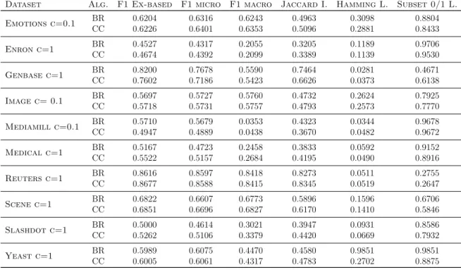
Results of Experiment 2 are shown in Table 3.4. Comparing these results with the ones obtained in Experiment 1 (Section 3.2.2), it is possible to observe that the obtained performance of BR for F1macro in relation with CC is much better in this experiment

than in the previous one. Results in Table 3.2 forF1macroare, in general, worse for BR

than for CC and in those data sets where BR obtains better performance, the results of both algorithms are almost equal. Nevertheless, in Table 3.4, BR obtains better results for F1macro measure than CC in almost the half of the data sets (genbase,

image, reuters and yeast), while in those ones for which CC has better performance, the numerical results are very near.

Specifically, if results for data set yeast are considered for F1macro, in Experiment 1,

CC obtained the best result while BR obtained the worst one, but, in Experiment 2, BR obtained a much better result than CC for the same measure. Another example is data set image; the results of BR in Experiment 1 were worse than the results obtained by CC, but in Experiment 2, BR obtained better performance than CC. Therefore, despite the limitations of this experiment, it is possible to observe, as it was supposed, that when F1 is optimized, BR optimizes F1macro and the results of this algorithm

for this measure tend to approach to the ones of CC and, in some cases, even improve them.

Section 3.3. Experiment 2: Optimizing F1

Table 3.4: Results of Experiment 2: Optimizing Hamming Loss.

Dataset Alg. F1 Ex-based F1 micro F1 macro Jaccard I. Hamming L. Subset 0/1 L. Emotions c=0.1 BR_CC 0₀._.6204_{6226 0}0._.64016316 ₀0_..6243₆₃₅₃ 0_0..₅₀₉₆4963 ₀0_..₂₈₈₁3098 ₀0_..8804₈₄₃₃ Enron c=1 BR_CC 0₀._.4527_{4674 0}0._.43924317 ₀0_..2055₂₀₉₉ 0_0..₃₃₈₉3205 ₀0_..₁₁₃₉1189 ₀0_..9706₉₅₃₀ Genbase c=1 BR_CC 0₀._.8200_{7602 0}0._.71867678 ₀0_..5590₅₄₂₃ 0_0..₆₆₂₆7464 ₀0_..₀₃₇₃0281 ₀0_..4671₆₁₃₈ Image c= 0.1 BR_CC 0₀._.5697_{5718 0}0._.57315727 ₀0_..5760₅₇₅₇ 0_0..₄₇₉₃4732 ₀0_..₂₅₇₃2624 ₀0_..7925₇₇₇₀ Mediamill c=0.1 BR_CC 0₀._.5710_{4947 0}0._.48895679 ₀0_..0353₀₄₃₈ 0_0..₃₆₇₀4323 ₀0_..₀₄₈₂0344 ₀0_..9678₉₆₇₂ Medical c=1 BR_CC 0₀._.5167_{5522 0}0._.51574723 ₀0_..2458₂₆₈₄ 0_0..₄₁₉₅3833 ₀0_..₀₄₉₀0592 ₀0_..9152₈₉₁₆ Reuters c=1 BR_CC 0₀._.8616_{8677 0}0._.85888597 ₀0_..8418₈₄₁₅ 0_0..₈₃₄₅8273 ₀0_..₀₅₁₉0511 ₀0_..2755₂₆₄₇ Scene c=1 BR_CC 0₀._.6822_{6851 0}0._.66966607 ₀0_..6773₆₈₂₇ 0_0..₆₁₇₀5896 ₀0_..₁₄₁₀1596 ₀0_..6706₅₈₄₆ Slashdot c=1 BR_CC 0₀._.5000_{5262 0}0._.51064614 ₀0_..3021₃₃₇₉ 0_0..₄₄₂₀3947 ₀0_..₀₆₆₉0931 ₀0_..8586₇₉₃₂ Yeast c=1 BR_CC 0₀._.5989_{6005 0}0._.60616075 ₀0_..4470₄₃₁₇ 0_0..₄₇₈₃4580 ₀0_..₂₇₀₂9851 ₀0_..9851₈₈₇₅

Chapter 4

Conclusions

4.1

Summary of contributions and results

A study of decomposition methods for multilabel classification has been developed in this project. Specifically, first of all, an introduction to multilabel classification was done, including the formal framework for this kind of problems and an exposition about several evaluation metrics that can be used to evaluate the performance of the algorithms employed to solve the problem. After that, different kinds of methods for multilabel classification were commented and a description, in more detail, of the decomposition methods that later were experimentally studied, was done. Apart from that, two more sections were included: the first one talking about label dependence and the other one commenting some tasks related to multilabel classification.

Once the more theoretical aspects were exposed, two experiments were done with the decomposition methods previously commented in Section 2.2.3. These experiments were carried out over various data sets with different properties (shown in Table 3.1). Global aim of both experiments was to compare the performance of BR (Binary Relevance) method in relation with other decomposition algorithms optimizing different evaluating metrics in each experiment. The aim of these experiments was motivated because, as it was also commented in this work, BR is a very simple algorithm with a lot of advantages but it is usually criticized due to the fact that it does not take into account dependences among labels. This makes the performance of BR be lower than the performance of the other algorithms but this study tries to demonstrate that these results are importantly affected by the way comparisons are made and the evaluation metrics used to evaluate the algorithms.

In this sense, in the first experiment, base classifiers were designed to optimize the accuraccy so the expected result was to obtain a BR which optimized Hamming Loss measure, while in the second experiment F1 was optimized so BR was expected to

optimize F1macro. An important aspect to have into account in second experiment

is that it was limited because of time restrictions so only BR and CC methods were analized and, unlike in the first experiment, no statistical tests were performed. Nevertheless, a trend was observed in the obtained results.

Chapter 4. Conclusions

Results of Experiment 1 verified that using base classifiers that optimize the accuraccy, BR optimizes Hamming Loss and obtains a competitive performance in this measure in relation to the rest of algorithms tested in the experiment. In relation to Experiment 2, despite its limitations, it was possible to observe that when F1 is optimized, BR

optimizes F1macroand the results of this method for this measure tend to approach to

the ones obtained by CC and, in some cases, improve them.

Apart from that, Experiment 1 also pursued the goal to analize the methods shown in Figure 2.1 in order to observe if it is better to use the actual labels or the predictions in the training phase and if it is preferable to employ all of them, like in STA and DBR methods, or only previous ones like in CC and NS methods. According to the obtained results, in general, it is better to use actual labels (CC and DBR methods) than predictions in the training phase although there are some measures (F1micro

and Hamming Loss) that are optimized by methods using predictions (NS and STA). In relation to use all previous labels or predictions or only previous ones, the results shown that this aspect does not really affect the performance.

4.2

Future work

The fact that STA and NS, which are methods that use predictions in the training phase, obtained the best performance for Hamming Loss in Experiment 1, should also be analized in more detail to look for a theorical explanation that supports this fact. Another good idea for future work would be extending Experiment 2 to include all the aspects that were cut out in this work due to time limitations. In particular, it would be advisable to include all methods shown in Figure 2.1 and employ a grid search to establish the values of the regularization parameterC for each binary model. Finally, as it was done in Experiment 1, a two-step statistical test procedure should be performed following the recommendations in [Demˇsar, 2006].

Bibliography

H. Blockeel, L. Schietgat, J. Struyf, S. Dˇzeroski, and A. Clare. Decision trees for hierarchical multilabel classification: A case study in functional genomics. Knowledge discovery in databases: PKDD 2006, pages 18–29, 2006.

M.R. Boutell, J. Luo, X. Shen, and C.M. Brown. Learning multi-label scene classification. Pattern recognition, 37(9):1757–1771, 2004.

K. Brinker, J. F¨urnkranz, and E. H¨ullermeier. A unified model for multilabel classification and ranking. In Proceeding of the 2006 conference on ECAI 2006: 17th European Conference on Artificial Intelligence August 29–September 1, 2006, Riva del Garda, Italy, pages 489–493. IOS Press, 2006.

R. Caruana. Multitask learning. Machine learning, 28(1):41–75, 1997.

N. Cesa-Bianchi, C. Gentile, and L. Zaniboni. Hierarchical classification: combining bayes with svm. In Proceedings of the 23rd international conference on Machine learning, pages 177–184. ACM, 2006.

W. Cheng and E. H¨ullermeier. Combining instance-based learning and logistic regression for multilabel classification. Machine Learning, 76(2-3):211–225, 2009. doi: 10.1007/s10994-009-5127-5. URL http://dx.doi.org/10.1007/ s10994-009-5127-5.

A. Clare and R. D. King. Knowledge discovery in multi-label phenotype data. In

European Conf. on Data Mining and Knowledge Discovery, pages 42–53, 2001. ISBN 3-540-42534-9. URL http://portal.acm.org/citation.cfm?id=645805.670013. F. De Comit´e, R. Gilleron, and M. Tommasi. Learning multi-label alternating decision

trees from texts and data.Machine Learning and Data Mining in Pattern Recognition, pages 251–274, 2003.

K. Dembczy´nski, W. Cheng, and E. H¨ullermeier. Bayes Optimal Multilabel Classification via Probabilistic Classifier Chains. In ICML, pages 279–286, 2010a.

K. Dembczy´nski, W. Waegeman, W. Cheng, and E. H¨ullermeier. Regret analysis for performance metrics in multi-label classification: the case of hamming and subset zero-one loss. In ECML’2010, Part I, pages 280–295. Springer, 2010b. ISBN 3-642-15879-X, 978-3-642-15879-7. URLhttp://portal.acm.org/citation.cfm?id= 1888258.1888284.

K. Dembczynski, W. Waegeman, W. Cheng, and E. H¨ullermeier. On label dependence in multi-label classification. In International conference on machine learning (ICML)-2nd international workshop on learning from multi-label data (MLD’2010), pages 5–12, 2010.

K. Dembczy´nski, W. Waegeman, W. Cheng, and E. H¨ullermeier. On label dependence and loss minimization in multi-label classification. Machine Learning, To appear, 2012.

J. Demˇsar. Statistical comparisons of classifiers over multiple data sets. Journal of Machine Learning Research, 7:1–30, 2006. ISSN 1532-4435.

S. Diplaris, G. Tsoumakas, P. Mitkas, and I. Vlahavas. Protein classification with multiple algorithms. Advances in Informatics, pages 448–456, 2005.

A. Elisseeff and J. Weston. A Kernel Method for Multi-Labelled Classification. In

ACM Conf. on Research and Develop. in Infor. Retrieval, pages 274–281, 2005. URL

http://citeseerx.ist.psu.edu/viewdoc/summary?doi=10.1.1.18.2423.

J. F¨urnkranz, E. H¨ullermeier, E. Loza Menc´ıa, and K. Brinker. Multilabel classification via calibrated label ranking. Machine Learning, 73:133–153, 2008. ISSN 0885-6125. doi: 10.1007/s10994-008-5064-8. URLhttp://portal.acm.org/citation.cfm?id= 1416930.1416934.

N. Ghamrawi and A. McCallum. Collective multi-label classification. InACM Int. Conf. on Information and Knowledge Management, pages 195–200. ACM, 2005. ISBN 1-59593-140-6. doi: http://doi.acm.org/10.1145/1099554.1099591. URL http://doi. acm.org/10.1145/1099554.1099591.

S. Godbole and S. Sarawagi. Discriminative methods for multi-labeled classification. In

Pacific-Asia Conf. on Know. Disc. and Data Mining, pages 22–30, 2004.

E. H¨ullermeier, J. F¨urnkranz, W. Cheng, and K. Brinker. Label ranking by learning pairwise preferences. Artificial Intelligence, 172(16-17):1897–1916, 2008.

R. Jin and Z. Ghahramani. Learning with multiple labels. Advances in Neural Information Processing Systems, 15:897–904, 2002.

T. Joachims. A support vector method for multivariate performance measures. In

Proceedings of the 22nd international conference on Machine learning, pages 377– 384. ACM, 2005.

T. Li and M. Ogihara. Detecting emotion in music. In Proceedings of the International Symposium on Music Information Retrieval, Washington DC, USA, pages 239–240, 2003.

T. Li and M. Ogihara. Toward intelligent music information retrieval. Multimedia, IEEE Transactions on, 8(3):564–574, 2006.

X. Luo and A. Zincir-Heywood. Evaluation of two systems on multi-class multi-label document classification. Foundations of Intelligent Systems, pages 234–253, 2005. O. Maron and T. Lozano-P´erez. A framework for multiple-instance learning. In

Advances in neural information processing systems, pages 570–576. MORGAN KAUFMANN PUBLISHERS, 1998.

A. K. McCallum. Multi-label text classification with a mixture model trained by em. In AAAI 99 Workshop on Text Learning, 1999.

E. Monta˜n´es, J. R. Quevedo, and J. J. del Coz. Aggregating independent and dependent models to learn multi-label classifiers. InProceedings of the 2011 European conference on Machine learning and knowledge discovery in databases - Volume Part II, ECML PKDD’11, pages 484–500, Berlin, Heidelberg, 2011. Springer-Verlag. ISBN 978-3-642-23782-9.

E. Montan´es, J.R. Quevedo, and J.J. del Coz. Una mejora de los modelos apilados para la clasificaci´on multi-etiqueta.

Guo J. Qi, Xian S. Hua, Yong Rui, Jinhui Tang, Tao Mei, and Hong J. Zhang. Correlative multi-label video annotation. In Proceedings of the International conference on Multimedia, pages 17–26, New York, NY, USA, 2007. ACM. ISBN 978-1-59593-702-5. doi: 10.1145/1291233.1291245. URL http://dx.doi.org/10. 1145/1291233.1291245.

J. Ram´on Quevedo, O. Luaces, and A. Bahamonde. Multilabel classifiers with a probabilistic thresholding strategy. Pattern Recognition, 2011.

J. Read. A pruned problem transformation method for multi-label classification. In

Proc. 2008 New Zealand Computer Science Research Student Conference (NZCSRS 2008), pages 143–150, 2008.

J. Read, B. Pfahringer, and G. Holmes. Multi-label classification using ensembles of pruned sets. In IEEE Int. Conf. on Data Mining, pages 995–1000. IEEE, 2008. ISBN 978-0-7695-3502-9. doi: 10.1109/ICDM.2008.74. URL http://portal.acm.org/ citation.cfm?id=1510528.1511358.

J. Read, B. Pfahringer, G. Holmes, and E. Frank. Classifier chains for multi-label classification. In ECML’09, LNCS, pages 254–269. Springer, 2009a. URL http: //dx.doi.org/10.1007/978-3-642-04174-7_17.

J. Read, B. Pfahringer, G. Holmes, and E. Frank. Classifier chains for multi-label classification. Machine Learning and Knowledge Discovery in Databases, pages 254– 269, 2009b.

J. Read, B. Pfahringer, G. Holmes, and E. Frank. Classifier chains for multi-label classification. Machine Learning, 85(3):333–359, 2011.

Robert E. Schapire and Yoram Singer. Boostexter: A boosting-based system for text categorization. In Machine Learning, pages 135–168, 2000.