TESIS DOCTORAL
Small area estimation methods under
complex sampling designs
Autor:
MARIA GUADARRAMA SANZ
Director:
Isabel Molina Peralta
DEPARTAMENTO DE ESTADÍSTICA
PH.D. THESIS
Small area estimation methods under
complex sampling designs
1
Author:
Mar´ıa Guadarrama Sanz
Advisor:Isabel Molina Peralta
DEPARTMENT OF STATISTICS
Getafe, Madrid, October 20, 2017
A PhD is no easy feat. This dissertation was made possible by the incredible people and organizations with whom I have had the pleasure of working with. Without each of them, my work would not have been possible or as rewarding as it has been.
Firstly, I would like to express my deepest gratitude to my advisor, Prof. Isabel Molina, for her guidance, patience, enthusiasm and immense knowledge which have provided me with a continuous stream of support throughout my PhD and research. Prof. Molina’s advice and support have been invaluable. I know for a fact that I could not have had a better advisor and mentor. Also, I am extremely grateful to Prof. Yves Till´e and Prof. J.N.K. Rao for making their endless knowledge available to me.
I also would like to thank my professors from the University of Valladolid who encouraged me to enter the research world, especially Professors Jes ´us Cavero, Jose Luis Rojo, Isabel G ´omez, Jes ´us Alonso and Pedro Pablo Ortu ˜nez. Similarly, I would like to express my gratitude to my professors from the Department of Statistics of Universidad Carlos III de Madrid, especially Professors Helena Veiga, Juan Miguel Mar´ın, Michael Wiper, Javier Prieto and Regina Kaiser. Thanks to the administratives Susana Linares, Francisco Garc´ıa-Saavedra and Almudena Crespo for making much easier what, without them, would have been administrative nightmares.
I am very grateful to all friends from my village, from Valladolid, as well as those in Getafe who have helped me through the bad times and celebrated with me in the good moments. In particular, I am grateful to Ana and her parents, who make me discover Madrid when I was very young. I thank Ainara and Sandra who, since years ago, have moved together with me and accompanied me during these important stages of my life. Lorena, Yessica and Pablo - friends who, although they may be far away from time to time, are always near in mind. To Pato, because she was my first and best roommate. To Noelia and Robert since they have supported me during these last steps. To colleagues in my department: Daniel and Francisco because four years in the same office deserves recognition; Mario, Diego, Ginette, Andr´es, Jo˜ao, Alba, Elisa, Antonio and Hoang, because together we learned that, when life gives you lemons, make lemonade! To the Getagroup girls and boys: Silvina, Luciana, Juliana, Shireen, Marta, Vanesa, C´arita, Facundo, Manu, David, Ab Zereei, Mehdi, Pedro, and Manuel,
because their company has been the very best of my stay in Getafe (as we all know, without Eskinazo, I would never have finished this thesis!).
I would be thoughtless not to express my gratitude to two persons that have been of tremendous help during these years I have been in Getafe: F´elix Sanz and Adela G ´omez. Without them, Saturday lunches would not have been the same. Moreover, I would like to thank all the people of Casa Regional de Castilla y Le´on en Getafe, who brought me a taste of home when I needed it most.
Last but not the least, I would like to thank my parents, whose support has been essential to me throughout my life - especially during my PhD. You taught me to always look forward and never give up. Thanks to the rest of my family: my aunts, uncles, cousins, and grandparents, who have always encouraged me. Grandpa, I miss you!
The aim of this thesis is the study of small area estimation methods under outcome-dependent sampling designs, that is, when the selection of the units to the sample depends on their values of the variable of interest. More precisely, we consider two types of informative sampling designs. A first type, in which the inclusion probabilities are strictly positive for all population units and a second type, cut-off sampling, in which a grouping variable related with the variable of interest divides the population in two strata, with one of the strata being deliverately excluded from selection to the sample, that is, where inclusion probabilities are zero. We are specially interested in the estimation of general non-linear parameters, including poverty indicators, in areas or domains of the population with small sample sizes. Due to the small area sample sizes, we will use model-based methods, which borrow strength from all the domains through the assumption of models with common parameters for all the domains.
First, we review the main model-based small area estimation methods for the estimation of general nonlinear parameters, focusing for illustration purposes on particular poverty indicators. We describe direct estimation, which uses data only of the area of study, the empirical best linear unbiased predictor (EBLUP) under the Fay-Herriot at area level model (Fay and Herriot, 1979) and three methods based on unit-level models, namely the method of Elbers et al.(2003) used traditionally by the World Bank, the empirical best/Bayes (EB) method of Molina and Rao(2010) and the hierarchical Bayes proposal ofMolina et al.(2014). We put ourselves in the point of view of a practitioner and discuss, as objectively as possible, the benefits and drawbacks of each method, illustrating some of them through simulation studies and also by an application with real data.
In one of the mentioned simulation experiments, we study the performance of the considered estimators under informative sampling. Under informative selection, individuals with certain outcome values appear more often in the sample and, as a consequence, usual inference based on the actual sample without appropriate weight-ing might be strongly biased. In this dissertation, we propose an extension of the EB method, called pseudo EB (PEB) method, for estimation of general non-linear
parameters in small areas that handles the informative selection by incorporating the sampling weights. We analyze the properties of this method under complex sampling designs, including informative selection. Results confirm that the PEB estimators reduce significantly the bias of unweighted EB estimators under informative sampling, and compare favorably under non-informative selection. We illustrate the procedure through an application to poverty mapping in a Mexican state.
Additionally, we study small area estimation methods under cut-off sampling. This sampling technique consists of excluding a set of units from the selection to the sample due to difficulty in obtaining information from them. In that situation, na¨ıve estimators, obtained by ignoring the cut-off sampling, may be severely design-biased. Calibration estimators using auxiliary information have been proposed to reduce this design-bias. However, the resulting estimators may have large variances when estimating in small domains. Similarly as calibration, model-based small area estimation methods might also help decreasing this bias if the assumed model holds for the whole population. At the same time, these methods provide more efficient estimators than calibration when estimating in small domains. We compare the performance of calibration estimators with the EBLUP or the EB predictors for estimation in small domains under cut-off sampling through simulation studies and a real data application. Our results confirm that the EBLUP under simple random sampling without replacement applied to the non-excluded units helps to reduce the bias due to cut-off sampling. The EBLUP also performs significantly better than na¨ıve direct and calibration estimators in terms of mean squared error. Our results with real data suggest similar conclusions for the EB estimators of nonlinear domain parameters.
List of Figures ix
List of Tables xiii
1 Introduction 1
1.1 Motivation . . . 1
1.2 Organization and outline of the thesis . . . 4
2 A comparison of SAE methods for poverty mapping 7 2.1 Poverty indicators . . . 8
2.2 Estimators . . . 8
2.2.1 Direct estimators . . . 9
2.2.2 Fay-Herriot model . . . 10
2.2.3 ELL method . . . 12
2.2.4 Empirical Best/Bayes (EB) method . . . 14
2.2.5 Hierarchical Bayes (HB) method . . . 17
2.3 Simulation studies . . . 20
2.3.1 Nested error model with simple random sampling . . . 20
2.3.2 Nested error model with informative sampling . . . 23
2.3.3 Nested error model with outliers . . . 26
2.4 Application Spanish SILC data . . . 28
3 SAE of general parameters under informative sampling 39 3.1 Population model . . . 40
3.2 Sample selection mechanism . . . 41
3.3 EB method . . . 42
3.4 Pseudo EB method . . . 45
3.5 Parametric bootstrap MSE estimator . . . 47
3.6 Simulation experiments . . . 48 v
3.6.1 Simulation study with non-informative selection. . . 48
3.6.2 Simulation study with informative selection . . . 50
3.7 Application to poverty mapping in Mexico . . . 55
4 SAE methods under cut-off sampling 67 4.1 Estimation of population totals or means . . . 68
4.1.1 Basic design-based estimators. . . 68
4.1.2 Calibration estimators . . . 69
4.2 Domain estimators . . . 71
4.2.1 Basic direct estimators . . . 71
4.2.2 Calibration estimators . . . 72
4.3 Small area estimation under cut-off sampling . . . 74
4.3.1 Direct calibration . . . 75
4.3.2 Calibration after reweighting . . . 77
4.3.3 Generalized calibration estimators . . . 78
4.3.4 EBLUP . . . 80
4.3.5 Empirical best predictor . . . 82
4.4 MSE estimation . . . 83
4.5 Simulation experiment . . . 84
4.6 Estimation of sales of tobacco products. . . 87
5 Conclusions and future research lines 93 5.1 Overall conclusions . . . 93
5.2 Future research lines . . . 95
Bibliography 97 A Proofs of Chapter 2 101 A.1 EBLUP . . . 101
A.2 Posterior distribution for HB . . . 102
B Proofs of Chapter 3 105 C Proofs of Chapter 4 109 C.1 Equality of basic calibration estimator and GREG . . . 109
C.2 Derivation of calibration functionF(·) . . . 109
C.3 Derivation of LCALN estimator . . . 110
C.4 Design-bias of LCAL estimator under cut-off sampling . . . 111
C.6 Properties of RWCAL estimator of domain total . . . 114
C.7 Derivation of generalized calibration weights . . . 115
C.8 Design-bias of BLUP of domain mean under cut-off sampling with
srswor within the set of included units . . . 115
C.9 Cut-off sampling versus srswor . . . 117
2.1 Percent RB (left) and RRMSE (right) of direct, FH, HB and ELL estimators
of poverty gapF1i for each domainiunder the nested error model with
srswor. . . 22
2.2 Percent RB (left) and RRMSE (right) of EB and Census EB estimators of
poverty gap F1i for each domain iunder the nested error model with
srswor. . . 23
2.3 True MSE of ELL estimators of poverty gapF1i and mean across
simu-lations of ELL estimator of the MSE for each domaini, under the nested
error model with srswor. . . 24
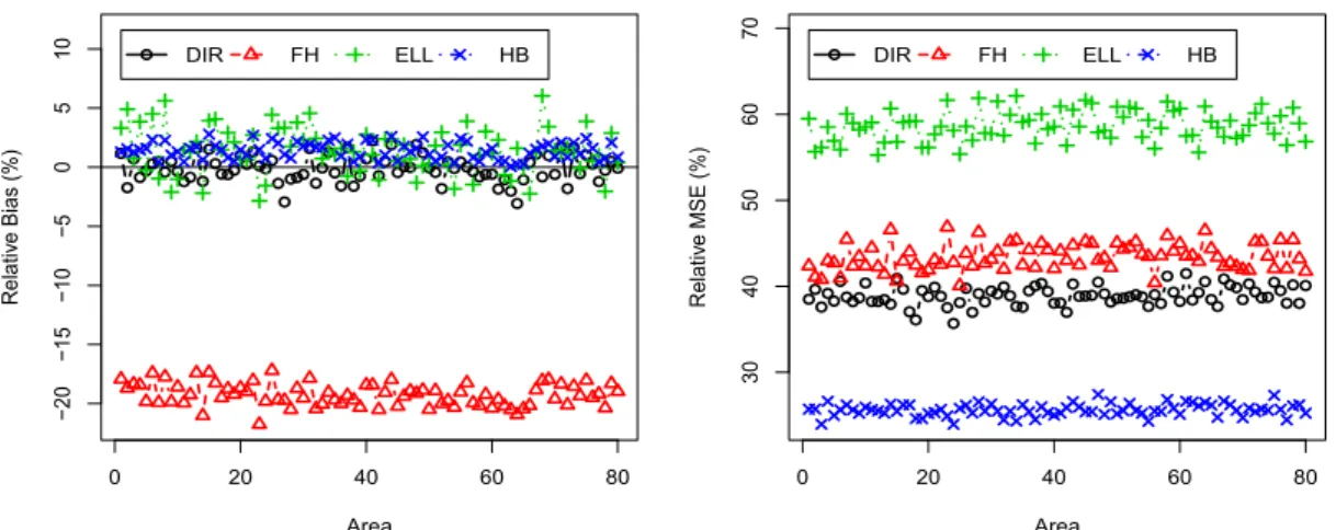
2.4 Percent RB (left) and RRMSE (right) of direct, FH, HB and ELL estimators
of poverty gapF1ifor each domainiunder low informativeness. . . 27
2.5 Percent RB (left) and RRMSE (right) of direct, FH, HB and ELL estimators
of poverty gapF1ifor each domainiunder high informativeness. . . 27
2.6 Percent RB (left) and RRMSE (right) of direct, FH, HB and ELL estimators
of poverty gap F1i for each domain i under nested error model with
outliers (p= 0.01andR= 10).. . . 29
2.7 Percent RB (left) and RRMSE (right) of direct, FH, HB and ELL estimators
of poverty gap F1i for each domain i under under nested error model
with outliers (p= 0.05andR= 100) . . . 30
2.8 Cartograms of estimated percent poverty incidences, Fˆ0i, in Spanish
provinces for women obtained with direct (top left), FH (top right) and
HB (bottom left) methods. . . 33
2.9 Cartograms of estimated percent poverty gaps,Fˆ1i, in Spanish provinces
for women obtained with direct (top left), FH (top right) and HB (bottom
left) methods. . . 34
2.10 Cartograms of estimated percent poverty incidences, Fˆ0i, in Spanish
provinces for men obtained with direct (top left), FH (top right) and HB
(bottom left) methods. . . 35
2.11 Cartograms of estimated percent poverty gaps,Fˆ1i, in Spanish provinces
for men obtained with direct (top left), FH (top right) and HB (bottom
left) methods. . . 36
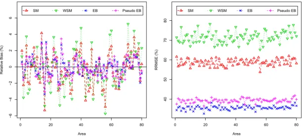
3.1 Percent RB (left) and RRMSE (right) of SM, WSM, EB and pseudo EB
estimators of poverty gap, F1i, for each area, under non-informative
selection withn¯i= 25. . . 51
3.2 Percent RB (left) and RRMSE (right) of SM, WSM, EB and pseudo EB
estimators of poverty gap, F1i, for each area, under non-informative
selection withn¯i= 50. . . 51
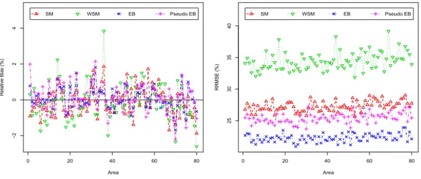
3.3 Percent RB (left) and RRMSE (right) of SM, WSM, EB and pseudo EB
estimators of poverty gap, F1i, for each area, under non-informative
selection withn¯i= 75. . . 52
3.4 Percent RB (left) and RRMSE (right) of SM, WSM, EB and pseudo EB
estimators of poverty gap,F1i, for each area, under informative selection,
¯
ni = 25. . . 53
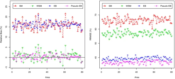
3.5 Percent RB (left) and RRMSE (right) of SM, WSM, EB and pseudo EB
estimators of poverty gap,F1i, for each area, under informative selection,
¯
ni = 50. . . 53
3.6 Percent RB (left) and RRMSE (right) of SM, WSM, EB and pseudo EB
estimators of poverty gap,F1i, for each area, under informative selection,
¯
ni = 75. . . 54
3.7 True MSEs of pseudo EB estimators of poverty gap, F1i, and expected
values of bootstrap MSE estimators with B = 500 bootstrap replicates,
for each domain.. . . 55
3.8 EB (left) and pseudo EB (right) residuals against predicted values. . . 58
3.9 Normal Q-Q plots of EB (left) residuals and pseudo EB (right) residuals. . 58
3.10 Normal Q-Q plot of EB (left) and pseudo EB (right) predicted
municipal-ity effects. . . 59
3.11 Unweighted direct estimates of poverty incidence (left) and poverty gap
(right) against weighted direct estimates for each sampled municipality. . 61
3.12 EB estimates of poverty incidence (left) and pseudo EB (right) against
weighted direct estimates for each sampled municipality. . . 61
3.13 EB (left) and pseudo EB (right) residuals against predicted values for
selected municipalities. . . 62
3.14 Normal Q-Q plot of EB residuals (left) and pseudo EB residuals (right)
3.15 Normal Q-Q plot of estimated effects by EB (left) and pseudo EB (right)
for each sampled municipalityi. . . 63
3.16 EB estimates of poverty incidence (left) and pseudo EB (right) against
weighted direct estimates for selected municipalites.. . . 63
3.17 Estimates (left) and coefficients of variation (right) of WSM, EB and
pseudo EB estimators of poverty incidence, F0i, for each selected
mu-nicipality. . . 64
3.18 Estimates (left) and coefficient of variation (right) of WSM, EB and
pseudo EB estimators of poverty gap,F1i, for each selected municipality. . 64
3.19 Cartograms of estimated percent poverty incidences,F0i, in the selected
municipalities from the State of Mexico, obtained with direct (top left),
EB (top right) and pseudo EB (bottom left) methods. . . 65
3.20 Cartograms of estimated percent poverty incidences,F1i, in the selected
municipalities from the State of Mexico, obtained with direct (top left),
EB (top right) and pseudo EB (bottom left) methods. . . 66
4.1 Percent RB (left) and RRMSE (right) of HT, LCAL, LCALN and EBLUP
estimators of domain mean,Y¯i, for each area. . . 86
4.2 EB residuals against predicted values (left), and histogram of EB
residu-als (right). . . 89
4.3 Normal Q-Q plot of predicted province effectsvˆi.. . . 90
4.4 EB estimates against direct estimates (left), and against GREG estimates
(right) for each province. . . 90
4.5 Direct, calibration and EB estimates of total sales of tobacco in Spanish
provinces (left). Estimated coefficient of variation of direct, calibration
2.1 Averages across domains of percent ARB and RRMSE for direct, FH, HB,
EB, Census EB and ELL estimators of poverty incidenceF0iand poverty
gapF1i, under the nested error model with srswor.. . . 23
2.2 Averages across domains of percent ARB and RRMSE for direct, FH, HB,
EB and ELL estimators of incidenceF0i and poverty gapF1i, under low
informativeness. . . 26
2.3 Averages across domains of percent ARB and RRMSE for direct, FH, HB,
EB and ELL estimators of incidenceF0iand poverty gapF1i, under high
informativeness. . . 26
2.4 Averages across domains of percent ARB and RRMSE for direct, FH, HB,
EB and ELL estimators of incidenceF0iand poverty gapF1i, under under
nested error model with outliers (p= 0.01andR= 10). . . 29
2.5 Averages across domains of percent ARB and RRMSE for direct, FH, HB,
EB and ELL estimators of incidenceF0iand poverty gapF1i, under under
nested error model with outliers (p= 0.05andR= 100). . . 30
2.6 Results for poverty incidences for women: Direct, FH and HB estimates
together with coefficients of variation (%) for Spanish provinces with
sample sizes closest to minimun, 0.25, 0.5, 0.75 quantiles and maximum. . 31
2.7 Results for poverty incidences for men: Direct, FH and HB estimates
together with coefficients of variation (%) for Spanish provinces with
sample sizes closest to minimum, 0.25, 0.5, 0.75 quantiles and maximum. . 31
2.8 Results for poverty gaps for women: Direct, FH and HB estimates
together with coefficients of variation (%) for Spanish provinces with
sample sizes closest to minimum, 0.25, 0.5, 0.75 quantiles and maximum. . 31
2.9 Results for poverty gaps for men: Direct, FH and HB estimates together
with coefficients of variation (%) for Spanish provinces with sample sizes
closest to minimum, 0.25, 0.5, 0.75 quantiles and maximum. . . 32
3.1 Averages across domains of percent absolute RB and RRMSE for SM,
WSM, EB and pseudo EB estimators of poverty incidence, F0i, and
poverty gap,F1i, under non-informative selection withn¯i = 25,50,75. . . 50
3.2 Averages across domains of percent absolute RB and RRMSE for SM,
WSM, EB and pseudo EB estimators of poverty incidence, F0i, and
poverty gap,F1i, under informative selection withn¯i= 25,50,75. . . 54
3.3 Test for sample ignorability. Code, sample size and observedF-value for
each selected municipality. . . 60
4.1 Averages across areas of percent absolute RB and RRMSE and average
B2π/MSEπfor HT, LCAL, LCALN and EBLUP (in percentage). . . 87
C.1 Direct, GREG and EB estimates of total sales for the selected product and estimated coefficients of variation (%) for each Spanish province. Results sorted by increasing sample size. . . 119
Introduction
1.1
Motivation
Poverty maps are an important source of information on the regional distribution of poverty and are currently used to support regional policy-making and to allocate funds to local jurisdictions. Good examples are the poverty and inequality maps produced by the World Bank for many countries all over the world. In the U.S., the Small Area Income and Poverty Estimates (SAIPE) program of the Census Bureau provides annual estimates of income and poverty statistics for all school districts, counties and states for the administration of federal, state and local programs and the allocation of federal funds to local jurisdictions (https://www.census.gov/did/www/saipe/). In Europe, the joint project “Poverty Mapping in the New Member States of the European Union” between the World Bank and the European Commission was aimed at constructing poverty maps for the new members of the EU. The TIPSE (Territorial Dimension of Poverty and Social Exclusion in Europe) project, commissioned by the European Observation Network for Territorial Development and Cohesion (ESPON) program, aims to support policy by creating a regional database and associated maps of poverty and social exclusion indicators. In Mexico, the National Council for the Assessment of Social Development Policy (CONEVAL in Spanish) is committed by law to produce regular poverty and inequality estimates at the state level by population subgroups and at municipality level. The first objective of the Sustainable Development Goals, substitutes of the former ”Millennium Objectives” of the United Nations (UN), is the end of poverty in all its forms everywhere. The UN propose eradicating extreme poverty for all people everywhere by 2030. As an indicator, the UN uses the proportion of population below the international poverty line (currently $1.25 per day) by sex, age, employment status and geographical location, both urban or rural, (https://sustainabledevelopment.un.org/sdg1).
Obtaining accurate poverty maps at high levels of disaggregation is not straightfor-ward because of insufficient sample size of official surveys in some of the target regions. Direct estimates, obtained with the region-specific sample data, are unstable in the sense of having very large sampling errors for regions with small sample size. These unstable poverty estimates might make the seemingly poorer regions in one period appear as the richer in the next period, which can be contradictory. On the other hand, very stable but biased estimates (e.g., too homogeneous across regions) might make identification of the poorer regions difficult.
Sample surveys are the primary data source for official statistics. However, the high cost of interviews leads to an extensive use of the survey data, including estimation for geographical levels (domains) for which they were not initially planned. As already said, when estimating for disaggregated domains, “direct” estimators, based only on the domain-specific sample data, can be highly inefficient because of small area-specific sample sizes. Domains where direct estimators do not have the required precision are called “small areas”. Small area estimation methods “borrow strength” by using “indirect” estimators that employ the sample data from other domains, leading to more efficient estimators. Among indirect estimation methods, model-based approaches, which combine survey data with other data sources such as censuses or administrative registers through linking models, are very popular because they can increase considerably the efficiency in very small areas. Pfeffermann et al. (2013) provides a recent review on the topic, and the book byRao and Molina(2015) contains a comprehensive description of small area estimation methods.
In small area estimation, models are typically classified into area level and unit level models. In area level models, direct area estimators are related to area level auxiliary variables. In unit level models, the values of the study variable for the population units are related to unit-specific covariates. Both unit and area level models have been used extensively to estimate linear parameters such as totals and means. However, many poverty and inequality indicators are complex nonlinear functions of the vector of values of the target variable (e.g. income) in the units of the domain of interest. Specific methods have been developed to address the estimation of general nonlinear parameters in small areas.
Area level models are widely used in official statistics applications. For instance, the U.S. Census Bureau uses the Fay-Herriot (FH) area level model (Fay and Herriot,
1979) to produce model-based county estimates of the number of school-age children under poverty. Molina and Morales(2015) also used the FH model to estimate poverty incidences and gaps in Spanish provinces. The first unit level model designed to estimate general non-linear parameters such as poverty indicators in small areas was
proposed byElbers et al.(2003), and will hereafter be called ELL method. This method has been extensively used by the World Bank to obtain disaggregated poverty and inequality maps of many countries. A more recent approach is the empirical best/Bayes (EB) method proposed by Molina and Rao (2010). This method also uses a unit level model and delivers the “best” (or optimal) estimator in the sense of minimizing the mean squared error (MSE) under the assumed model. Molina et al. (2014) have proposed a hierarchical Bayes (HB) analogue to the EB method to estimate general non-linear parameters in small areas.
In many applications, individuals with certain outcome values are more likely selected for the sample. For example, in forestry, the largest trees may be more likely to be selected; in case-control studies, cases are typically selected with larger probability than controls. In such situations, we say that the selection mechanism (or sampling design) is informative. The result of an informative selection is a sample that “without appropriate weighting” is not representative of the target population. In this situation, estimators which do not take into account the design weights may display large bias. Thus, a weighting procedure is needed to downweight the outcomes of individuals that appear more often in the sample. This is the idea of design-based estimation, where the Horvitz-Thompson estimator (Horvitz and Thompson, 1952), also called “expansion estimator” and the Haj´ek estimator (H´ajek, 1971), which is simply the weighted sample mean (WSM), are the basic estimators of a population mean. These design-based estimators do not require model assumptions and are consistent under general sampling mechanisms as the sample size becomes large. Model-based methods that are obtained ignoring the sampling weights, such as the EBLUP and the EB, may display a large bias under informative selection.
An extreme type of informative selection is cut-off sampling, where a set of population units are not accounted for the selection of the sample. This type of sampling is employed in many business surveys, where small firms are excluded from the sample because of the high cost of obtaining and maintaining a frame covering the whole population of firms. According to S¨arndal et al. (1992), pp. 531-533, this sampling technique is used when the distribution of the study variable is highly skewed and there is not a reliable frame covering the small elements. Benedetti et al.(2010) enumerate the practical advantages of cut-off sampling in terms of the survey reduction cost. The monthly survey of manufacturing performed by Statistics Canada is an example of cut-off sampling (Benedetti et al., 2010). In Spain, the monthly survey of industrial production index (IPI) performed by the Spanish National Statistical Institute (in Spanish, INE) collects data from those firms which produce a significant volume of products according to the annual industrial survey of products (in Spanish, EIAP), see
http://www.ine.es/daco/daco43/metoipi10.pdf. Related surveys, e.g. the Index of Industrial Prices (IIP) and the Index of Business Turnover (IBT) also use this sampling technique.
Cut-off sampling leads to biased estimates since the inclusion probabilities for excluded units are zero. Consecuently, the sampling weights for those units do not exist, see e.g. S¨arndal et al.(1992) andHaziza et al.(2010) among others. Haziza et al.
(2010) propose to use auxiliary information either at the design or at the estimation stage in order to reduce the bias when estimating population totals; more specifically, they propose to use balanced sampling or calibration, or both. Here, we restrict ourselves to the estimation stage. At this stage, Haziza et al. (2010) propose to use auxiliary information through calibration. Calibration estimators, or generalized regression (GREG) estimators, provide good results in terms of reduction of bias and efficiency when estimating at national level or at low levels of dissagregation where the sample size is large enough. However, for domains with small sample size, calibration estimators fail in terms of efficiency, displaying large variances. Model-based small area estimation methods, which use auxiliary information as well, reduce the bias due to cut-off sampling similarly as calibration. Moreover, because of the increase of the “effective” sample size, small area estimators help to reduce the variance in domains with small sample sizes. Furthermore, these methods allow the estimation of more complex parameters.
1.2
Organization and outline of the thesis
The Ph. Dissertation is organized as follows. In Chapter2, we review the main methods for estimation of general parameters in small areas. We consider estimators based on area level models such as Fay Herriot model (Fay and Herriot, 1979) and estimators based on unit level models, such as ELL method ofElbers et al.(2003), the best/Bayes estimator (EB) of Molina and Rao (2010), and the hierarchical Bayes estimator (HB)
of Molina et al. (2014). We comment on the advantages and disadvantages of these
methods from a practical point of view, illustrating them through simulation studies under different scenarios. First, we consider the case of the sample drawn by simple random sampling without replacement (srswor), then the case of informative sampling with different degrees of informativeness and, finally, we illustrate the case when outliers with different levels and intensities are present in the data. We construct poverty maps of Spain by provinces.
Chapter 3 is concerned with our proposed approach to reduce the bias due to informative selection of the sample. Since the bias showed by the unweighted
estimators such as EB is due to ignoring the sampling mechanism, we propose a weighted version of EB method, called pseudo EB (PEB). This procedure is based on the same conditioning idea of EB, but in this case we condition on the domain weighted sample mean (WSM). Simulation studies indicate a large reduction of the relative bias and good performance in terms of efficiency of pseudo EB estimators compared to EB. We prove the approximately design consistency of the PEB estimators of poverty incidence and gap. We illustrate the use of the proposed method estimating the poverty incidence and gap for municipalities of the State of Mexico.
Chapter4deals with cut-off sampling. We compare the already existing proposals with small area estimation methods. The main characteristic of cut-off sampling is that part of the population is excluded from possible sample selection. Na¨ıve estimators obtained by ignoring this fact lead to biased estimators. The solutions proposed so far, which use auxiliary information through calibration, may show large variances when estimating in small domains. We propose small area estimation methods to gain efficiency. Precisely, we consider the EBLUP in the case of linear parameters and the EB estimator for more general parameters. We compare the performance of calibration and the mentioned small area estimation methods through simulation studies. Results show that EBLUP and calibration estimates significantly reduce the bias of direct estimators due to cut-off sampling but, in terms of efficiency, calibration estimators exhibit large mean squared error in areas with small sample sizes. We use calibration and EB estimators to estimate the total sales of a specific tobacco product in Spanish provinces. Finally, Chapter5draws some conclusions from the thesis and proposes future research lines.
To make it easy for the reader, we have tried to make each chapter completely self-contained even if falling in the danger of becoming repetitive. Concerning notation, Chapters2-3try to follow the same notation, but some notation is changed in Chapter
4, trying to respect the conventional notation of related books and manuscripts. Even if some of the symbols have different meaning as in previous chapters, every symbol in this chapter is newly defined and we believe that all concepts are thus kept clear.
A comparison of small area
estimation methods for poverty
mapping
In the literature, we can find many different indicators describing wellbeing of people. The FGT class of poverty indicators introduced by Foster et al. (1984) includes basic indicators such as the at-risk-of-poverty rate, also called poverty incidence and defined as the proportion of individuals with welfare below the poverty line and the poverty gap defined as the mean relative distance to the poverty line. Poverty indicators that do not require definition of a poverty line are the Sen Index, Fuzzy monetary and Fuzzy supplementary poverty indicators (Betti et al.,2006). Inequality measures include Quintile Share Ratio, Gini index, Theil index, the Generalized entropy class (Theil index belongs to this class) and Atkinson’s inequality measures. For a description of these measures see e.g. Neri et al. (2005). As part of the Lisbon strategy of 2000, which envisioned the coordination of European social policies at country level based on a set of common goals, the European Council of Dec. 2001 established a set of common European statistical indicators on poverty and social exclusion called Laeken indicators
(Stubbs et al.,2008). This set contains several of the indicators mentioned above like the
at-risk-of-poverty rate, the Quintile Share Ratio and Gini index.
In this chapter, we review the main methods for the estimation of general non-linear small domain parameters, focusing for illustrative purposes on the FGT family of poverty indicators, which is introduced in Section 2.1. Specifically, in Section2.2, we describe direct estimation, the EBLUP based on the Fay and Herriot (1979) area level model used by the U.S. Census Bureau, the method ofElbers et al. (2003) used by the World Bank, the more recent empirical Best/Bayes (EB) method of Molina and Rao
(2010) together with its variation called Census EB, and the hierarchical Bayes (HB) method of Molina et al. (2014). We discuss advantages and disadvantages of each procedure from a practical point of view. In Section2.3, we illustrate their performance in simulations under several scenarios, including the cases of informative sampling or the presence of outliers. Finally, Section2.4applies several of the introduced procedures to poverty mapping in Spanish provinces by gender.
2.1
Poverty indicators
Although the methods reviewed in this chapter can be applied to many different poverty and inequality indicators, for simplicity of exposition and illustrative purposes, we will focus on the FGT family of poverty indicators. Consider a populationU of size
Nthat is partitioned intomdomains or areasU1, . . . , Um, of sizesN1, . . . , Nm. LetEij be
a measure of welfare for individualj(j = 1, . . . , Ni) in domaini(i= 1, . . . , m). Letzbe
the poverty line, that is, the value such that whenEij < z, individualjfrom domainiis
regarded as “at risk of poverty”. Then, the FGT family of poverty indicators for domain
iis given by Fαi = 1 Ni Ni X j=1 z−Eij z α I(Eij < z), α≥0, i= 1, . . . , m, (2.1)
where I(Eij < z) = 1 if Eij < z and I(Eij < z) = 0 otherwise. For α = 0, we
obtain the proportion of individuals “at risk of poverty”, that is, the poverty incidence or at-risk-of-poverty rate. For α = 1, we get the average of the relative distances to non being “at risk of poverty”, called poverty gap. The poverty incidence measures the frequency of poverty, whereas the poverty gap measures the intensity of poverty.
We remark that the unit level methods introduced in this chapter can be applied to estimate any desired population characteristic that is obtained as a real measurable function of the values of a continuous variable in the units of the population, as long as this variable follows the considered model in each method.
2.2
Estimators
Estimation of population characteristics is typically based on a samplesdrawn from the populationU. We denote bysi =s∩Ui the subsample from domainiof sizeni < Ni
and byri = Ui −si the complement of si, of size Ni−ni. The overall sample size is
n = Pm
i=1ni, i = 1, . . . , m. The following subsections describe common estimators of
2.2.1 Direct estimators
When estimating in a given domain or area i, a direct estimator uses only the ni
observations from that domain, provided that this domain has been sampled (i.e.,
ni > 0). The FGT poverty indicator (2.1) of order α for domain i can be expressed
as a mean as follows Fαi =Ni−1 Ni X j=1 Fαij, Fαij = z−Eij z α I(Eij < z), j= 1, . . . , Ni.
Since Fαi is now a mean of the domain elements Fαij, we can easily obtain the
Horwitz-Thompson (HT) direct estimator ofFαi as
ˆ
Fαi =Ni−1 X
j∈si
wijFαij, (2.2)
where wij = πij−1 is the sampling weight of unit j from domain i and πij is the
inclusion probability of unit j in the subsamplesi. The idea of the HT estimator (2.2)
is to downweight observations with larger probability of appearing in the sample and upweight those with smaller probability. Under the assumption that the second-order inclusion probabilities within domaini,πijl, satisfyπijl=πijπli,j6=l, which holds exactly under Poisson sampling within domain i, a design-unbiased estimator of the design variance ofFˆαi,Vˆπ( ˆFαi), is given by,
ˆ
Vπ( ˆFαi) =Ni−2 X
j∈si
wij(wij −1)Fαij2 . (2.3)
Below, we list the advantages and disadvantages of direct estimators, such as the HT estimator (2.2), for small area estimation.
Advantages:
• They are (at least approximately) design-unbiased and design-consistent asni →
∞. Thus, they perform well under complex sampling designs, including in-formative sampling, as long as they are calculated using the correct inclusion probabilities.
• They do not require model assumptions; that is, direct estimators are completely nonparametric.
Disadvantages:
• They cannot be calculated for nonsampled domains (i.e., withni = 0).
2.2.2 Fay-Herriot model
FH area level model was introduced byFay and Herriot (1979) and is currently used by the U.S. Census Bureau within the Small Area Income and Poverty Estimates (SAIPE) program (https://www.census.gov/did/www/saipe/). This model links the parameters of interest for all the domains,Fαi,i= 1, . . . , m, through a linear model as
Fαi=x0iβ+vi, i= 1, . . . , m, (2.4)
wherexiis ap-vector of area level covariates,βis the regression parameter common for
all domains, andviis the domain-specific regression error measuring the unexplained
domain heterogeneity and also called random effect for domain i. We assume that domain random effects vi are independent and identically distributed (iid), with
unknown varianceσv2, that is,vi iid
∼(0, σ2v). Note that true valuesFαiare not observable
and therefore model (2.4) cannot be directly fitted. However, we can make use of a direct estimatorFˆαi ofFαi. FH model assumes thatFˆαiis design-unbiased, with
ˆ
Fαi =Fαi+ei, i= 1, . . . , m, (2.5)
where ei is the sampling error for domaini. We assume that sampling errors ei are
independent of domain effectsviand satisfyeiind∼ (0, ψi), where the sampling variances
ψi,i= 1, . . . , m, are assumed to be known. Combining (2.4) and (2.5), we obtain a linear
mixed model
ˆ
Fαi =x0iβ+vi+ei, i= 1, . . . , m. (2.6)
The best linear unbiased predictor (BLUP) of Fαi = x0iβ+vi under model (2.6) is
simply obtained by fitting model (2.6) and replacing the estimate ofβand the predictor ofvi in (2.6), that is, the BLUP ofFαi is given by
˜
FαiF H =x0iβ˜+ ˜vi, (2.7)
where˜vi =γi( ˆFαj −x0iβ˜)is the BLUP ofvi, withγi =σv2/(σv2+ψi)and whereβ˜is the
weighted least squares estimator ofβ, given by
˜ β= m X i=1 γixix0i !−1 m X i=1 γixiFˆαi.
see AppendixA.1. In practice, the varianceσv2of the domain effectsviis unknown and
needs to be estimated. Common estimation methods are maximum likelihood (ML) and restricted maximum likelihood (REML). REML corrects for the degrees of freedom due to estimatingβand leads to a less biased estimator ofσv2for finite sample sizen. Letσˆv2
be the resulting estimator. Replacingσˆv2 forσ2v in (2.7), we obtain the empirical BLUP (EBLUP) of Fαi based on FH model (2.6), denoted here as FˆαiF H and called simply FH
estimator. Under normality ofvi andei, an approximation up too(m−1) terms for the
MSE of the FH estimator was obtained byPrasad and Rao(1990) and is given by MSE( ˆFαiF H) =gi1(σv2) +gi2(σv2) +gi3(σv2), where g1i(σ2v) = γiψi, g2i(σ2v) = (1−γi)2x0i m X i=1 γixix0i !−1 xi, g3i(σ2v) = (1−γi)2(σ2v+ψi2) −1V¯ π(ˆσ2v).
Here, V¯π(ˆσ2v) is the asymptotic variance of the estimator σˆ2v of σ2v under the assumed
model in this case (2.6).
Good and bad properties of FH estimator (2.7) are listed below, including particular properties for poverty mapping.
Advantages:
• The BLUP under FH model can be expressed as a weighted combination of the direct and the regression-synthetic estimators, that is,
˜
FαiF H =γiFˆαi+ (1−γi)x0iβ˜, i= 1, . . . , m. (2.8)
with weightγi =σ2v/(σv2+ψi). Then, for a domainiin which the direct estimator
ˆ
Fαi is inefficient, that is, with a large sampling variance ψi compared to the
unexplained between-domain variabilityσ2v,γi becomes small andF˜αiF H borrows
more strength from the other domains through the regression synthetic estimator
x0iβ˜. On the other hand, for a domain i in which the direct estimator Fˆαi is
efficient, that is, with small sampling variance ψi compared to the unexplained
between-domain variability σ2v, γi is large and F˜αiF H attaches more weight to
the direct estimator. Thus, FH estimator automatically borrows strength for the domains where it is actually needed.
• Ifγi >0for domaini, it makes use of the sampling weightswijthrough the direct
estimatorFˆαi. Thus, it is design-consistent asni → ∞. As a consequence, it is less
affected by informative sampling provided that the direct estimator is calculated using the correct inclusion probabilities.
• Due to the aggregation of data, it is not very much affected by isolated unit level outliers.
• It requires only domain level auxiliary information and therefore avoids the confidentiality issues associated with micro-data.
Disadvantages:
• The sampling variances ψi are assumed to be known, but in practice they are
estimated. It is not easy to incorporate the uncertainty due to estimation of the sampling variances in the MSE.
• The number of observations used to fit the FH model is the number of domainsm, which is typically much smaller than the number of observations used to fit unit level models,n. Thus, model parameters are estimated with less efficiency and, therefore, the efficiency gains with respect to direct estimators are expected to be smaller than under unit level models.
• It requires normality ofviandeifor MSE estimation. This might not hold for very
complex poverty indicators.
• If we want to estimate several indicators depending on a common continuous variable, it requires separate modeling and searching for good covariates for each indicator.
• Once the model is fitted at the domain level, small area estimatesFˆαiF H cannot be further disaggregated for subdomains or subareas within the domains unless a new good model is found at that subdomain level.
2.2.3 ELL method
ELL method assumes a unit level linear mixed model for a log-transformation of the variable measuring welfare of individuals, with random effects for the sampling clusters or primary sampling units. For comparability with the rest of the methods presented here, in the following, we assume that the sampling clusters are the domains. In this case, the model becomes the nested error model of Battese et al. (1988) for the log-transformation of the welfare variables, that is, Yij = log(Eij) is assumed
unit-specific and domain-specific covariates. The model also includes random area effectsvias follows
Yij =x0ijβ+vi+eij, j = 1, . . . , Ni, i= 1, . . . , m. (2.9)
Here, β is a p-vector of regression coefficients, vi iid
∼ (0, σ2v), eij ind
∼ (0, σe2k2ij)
where vi andeij are independent, and kij are known constants that may account for
heteroscedasticity.
ELL estimator ofFαiis given by the marginal expectation under model (2.9)FˆαiELL=
Em[Fαi]. This estimator, together with its MSE under model (2.9), are approximated by
a bootstrap method. In this bootstrap procedure, random effectsvi∗ and model errors
e∗ij are generated from residuals obtained by fitting model (2.9) to survey data. Then, a bootstrap census ofY-values is generated as
Yij∗=x0ijβˆ+vi∗+e∗ij, j= 1, . . . , Ni, i= 1, . . . , m,
whereβˆis an estimator ofβ. The generation is repeated fora = 1, . . . , A, obtainingA
censuses. Then, for each bootstrap censusa, the FGT poverty indicator for domainiis calculated as Fαi∗(a)= 1 Ni Ni X j=1 z−exp(Yij∗(a)) z !α I(exp(Yij∗(a))< z).
The ELL estimator of Fαi is then approximated by averaging over the A generated
censuses, that is,
ˆ FαiELL= 1 A A X a=1 Fαi∗(a).
The MSE of FˆαiELL under model (2.9), MSEm( ˆFαiELL), is then estimated in Elbers et al.
(2003) as follows
msem( ˆFαiELL) =
1 A A X a=1
Fαi∗(a)−FˆαiELL
2
. (2.10)
Advantages and disadvantages of ELL method are listed below: Advantages:
• It is based on unit level data, which are richer than area level data and typically uses much larger sample size (ncompared tom) to fit the model.
• ELL method can be applied to estimate general indicators defined as function of the model response variablesYij.
• They are model-unbiased if the model parameters are known.
• Once the model is fitted, estimates can be obtained at whatever subdomain level. Disadvantages:
• In terms of model MSE, ELL estimates perform poorly and can even perform worse than direct estimators when unexplained between-domain variation is significant, see Molina and Rao (2010). In fact, for the estimation of domain means, ELL estimates are basically equal to regression-synthetic estimators, which assume the regression model without further between-domain variation.
• They are based on a model assumption. Hence, model checking is crucial.
• They are not design-unbiased and can be seriously biased under informative sampling.
• They can be seriously affected by unit level outliers.
• If cluster effects are included in the model instead of area effects, but area effects are significant, ELL estimates of the model MSE can seriously underestimate the true MSE. Even if area effects are included in the model, ELL estimates of MSE do not track correctly the true model MSE for each domain.
2.2.4 Empirical Best/Bayes (EB) method
The EB method of Molina and Rao (2010) assumes that the population variables Yij
follow the nested error model (2.9) with normality of random effectsvi and errorseij.
Under that model, the domain vectors yi = (Yi1, . . . , YiNi)
0 are independent for i =
1, . . . , mand satisfyyi ind∼ N(µi,Vi), whereµi =Xiβ,Xi = (xi1, . . . ,xiNi)
0 andV i = σ2 v1Ni1 0 Ni+σ 2
eAi, forAi =diag(k2ij;j= 1, . . . , Ni). For a domain parameterHi =h(yi),
the estimator that minimizes the MSE, called the best estimator, is given by
˜
HiB =Eyir[h(yi)|yis;θ] = Z
h(yi)f(yir|yis;θ)dyir, (2.11)
wheref(yir|yis;θ)is the conditional probability density function (pdf) of the vectoryir
of out-of-sample values,Yij,j ∈ri, from domainigiven the vectoryisof sample values,
Yij,j ∈rifrom domaini, andθis the vector of model parameters. Now replacingθin
Under the nested error model (2.9), the distribution ofyir|yisis easy to derive. First,
we decompose Xi andVi into sample and out-of-sample elements similarly as we do
withyi, that is,
yi = yis yir ! , Xi= Xis Xir ! , Vi = Vis Visr Virs Vir ! .
By the normality assumption, we have that yir|yis ind∼ N(µir|s,Vir|s), where the
conditional mean vector and covariance matrix are given by
µir|s=Xirβ+γic(¯yic−x¯0icβ)1Ni−ni, (2.12) Vir|s=σv2(1−γi)1Ni−ni1 0 Ni−ni+σ 2 ediagj∈ri(k 2 ij). (2.13)
Here, γic = σ2v(σv2 +σe2/ci·)−1, for ci· = Pj∈sicij with cij = k −2
ij , andy¯ic and ¯xic are
weighted sample means obtained as
¯ yic = 1 ci· X j∈si cijYij, x¯ic = 1 ci· X j∈si cijxij. (2.14)
In practice, for complex non-linear parametersHi =h(yi), the expectation given in
(2.11) cannot be calculated analytically and it is approximated by Monte Carlo. This requires to simulate multivariate Normal vectors y(ira) of sizes Ni −ni, i = 1, . . . , m,
from the (estimated) conditional distribution of yir|yis and then to replicate for a =
1, . . . , A, which may be computationally unfeasible. This can be avoided by noting that the conditional covariance matrixVir|s, given by (2.13), corresponds to the covariance
matrix of a random vectory(ira)generated from the model
y(ira)=µir|s+v
(a)
i 1Ni−ni+
(a)
ir , (2.15)
wherevi(a)and(ira)are independent and satisfy
vi(a)∼N(0, σv2(1−γic)) and (a) ir ∼N(0Ni−ni, σ 2 ediagj∈ri(k 2 ij));
see Molina and Rao (2010). Using model (2.15), instead of generating a multivariate
normal vector yir(a) of sizeNi−ni, we just need to generate 1 +Ni−ni independent
univariate normal variablesvi(a) ind∼ N(0, σv2(1−γi))andij(a) ind∼ N(0, σ2ekij2), forj ∈ri.
Then, we obtain the corresponding out-of-sample valuesYij(a),j∈ri, from (2.15) using
as means, the corresponding elementsµij|sofµir|sgiven by (2.12). Using the vectory
(a)
ir
the parameter of interestHi(a)=h(yi(a)). For a non-sampled domaini(i.e., withni = 0),
we generateyir(a)from (2.15) withγic= 0and in this casey(ia) =y(ira). The Monte Carlo
approximation to the EB estimator (2.11) ofHi=h(yi)is then given by
ˆ HiEB ≈ 1 A A X a=1 h(y(ia)). (2.16)
In particular, to estimate the FGT poverty indicator given in (2.1),Molina and Rao
(2010) assumed thatYij = T(Eij)follow the nested error model (2.9), whereYij is the
transformed welfare andT(·)is a one-to-one transformation. In terms of the vector of transformed variablesyi = (Yi1, . . . , YiNi)
0, the FGT poverty indicator can be expressed
as Fαi = 1 Ni Ni X j=1 z−T−1(Yij) z α I(T−1(Yij)< z) =hα(yi), (2.17)
and the above EB method can be applied to the domain parameterHi=hα(yi).
In the case of complex parameters such as the FGT poverty indicators, analytic approximations for the MSE are hard to derive.Molina and Rao(2010) obtained a para-metric boostrap MSE estimator following the bootstrap method for finite populations
ofGonz´alez-Manteiga et al.(2008), seeMolina and Rao(2010) for further details.
Note that both ELL and EB methods require a survey data file containing the observations from the target variable and the auxiliary variables, that is,{(Yij,xij);j ∈
si, i = 1, . . . , m}, and a census containing the values of the same auxiliary variables
for all the units in the population, that is, {xij;j = 1, . . . , Ni, i = 1, . . . , m}. EB
method requires additionally to identify the set of out-of-sample unitsr(or equivalently the sample units s) in the census U. Linking the survey and the census files is not always possible in practice. However, typically the domain sample size ni is really
small compared to the population sizeNi. Then, we can use the Census EB estimator
described in Guadarrama et al. (2016), and obtained by generating in each Monte Carlo replicate the full census vector yi rather than only the vector of out-of-sample
observationsyir. For this, we apply the Monte Carlo approximation (2.16) by generating
y(ia) = µi|s +v (a) i 1Ni−ni + (a) i , where µi|s = Xiβ + γic(¯yic − ¯x0icβ)1Ni and (a) i ∼ N(0Ni, σ 2 ediagj=1,...,Ni(k 2
ij)). If the sampling fractionni/Ni is negligible, the Census EB
estimator ofHi =Fαiis practically the same as the original EB estimator.
Good properties and drawbacks of the EB method are listed below. Advantages:
much larger sample size to fit the model.
• EB method can be applied to estimate general indicators defined as functions of the response variablesYij.
• Best estimators are exactly model-unbiased.
• EB estimators are optimal in terms of minimizing the model MSE for known values of model parameters.
• EB estimators perform significantly better than ELL estimates when unexplained between-domain variation is significant. For out-of-sample domains (withni =
0), EB and ELL small area estimates are nearly the same. They are nearly the same for all domains if there is no unexplained between-domain variation (σ2v = 0).
• Once the model is fitted, estimates can be obtained at whatever subdomain level. Disadvantages:
• They are based on a model assumption. Hence, model checking is crucial.
• They are not approximately design-unbiased and can be seriously biased under informative sampling.
• They can be severely affected by unit level outliers.
• Parametric bootstrap estimates of the MSE of EB estimators are computationally intensive.
2.2.5 Hierarchical Bayes (HB) method
Computation of EB (and Census EB) estimates supplemented with their MSE estimates is very intensive and might be unfeasible for very large populations or for very complex indicators. Note that to approximate the EB estimate by Monte Carlo, we need to construct a large number A of censuses y(a), where each one might be of huge size. Moreover, to obtain the parametric bootstrap MSE estimator, the Monte Carlo approximation needs to be repeated for each bootstrap replicate. Seeking for a computationally more efficient approach,Molina et al.(2014) developed the alternative HB method for estimation of complex non-linear parameters. This approach does not require the use of bootstrap for MSE estimation because it provides samples from the posterior distribution, from which posterior variances play the role of MSEs, and any other useful posterior summary can be easily obtained.
The HB method is based on reparameterizing the nested error model (2.9) in terms of the intraclass correlation coefficient ρ = σv2/(σ2v +σe2) and considering only
non-informative priors for the model parameters(β, ρ, σe2). Concretely, the HB model is defined as (i) Yij|vi,β, σ2e, ρ ind ∼ N(x0ijβ+vi, σ2ek2ij), j= 1, . . . , Ni, (ii) vi|ρ, σe2 iid ∼ N 0, ρ 1−ρσ 2 e , i= 1, . . . , m, (iii) π(β, ρ, σe2)∝ 1 σ2 e , ≤ρ≤1−, σe2 >0,β∈ Rp, for >0small.
The posterior distribution can be obtained in terms of posterior conditionals using the chain rule of probability as follows. First note that, under the HB approach, the random effectsv= (v1, . . . , vm)0are regarded as additional parameters. Then, the joint
posterior pdf of the vector of parametersθ = (v0,β0, σ2e, ρ)0given the sample valuesys
is given by
π(v,β, σe2, ρ|ys) = π1(v|β, σe2, ρ,ys)π2(β|σe2, ρ,ys)π3(σ2e|ρ,ys)π4(ρ|ys), (2.18)
where the conditional pdfsπ1, . . . , π3have known forms, but notπ4(see AppendixA.2). However, sinceρis in a closed interval from(0,1), we can generate values fromπ4using a grid method, for more details seeMolina et al.(2014). Samples fromθ= (v0,β0, σ2e, ρ)0
can then be generated directly from the posterior distribution in (2.18), avoiding the use of Markov Chain Monte Carlo (MCMC) methods. Under general conditions, a proper posterior distribution is guaranteed, seeMolina et al.(2014).
Givenθ, population variablesYij are all independent, satisfying
Yij|θind∼ N(x0ijβ+vi, σe2k2ij), j= 1, . . . , Ni, i= 1, . . . , m. (2.19)
Consider the decomposition of the domain vector yi = (Yi1, . . . , YiNi)
0 in terms of
sample and out-of-sample elements yi = (y0is,y0ir)0. The posterior predictive pdf of
yiris then given by f(yir|ys) = Z Y j∈ri f(Yij|θ)π(θ|ys)dθ.
Finally, the HB estimator of a domain parameterHi =h(yi)is given by
ˆ
HiHB =Eyir(Hi|ys) = Z
h(yi)f(yir|ys)dyir. (2.20)
The HB estimator can be approximated by Monte Carlo. For this, we first generate samples from the posterior π(θ|ys) given in (2.18). We generate a value ρ(a) from
π4(ρ|ys) using a grid method; then, a value σ2(ea) is generated from π3(σ2e|ρ(a),ys);
next β(a) is generated from π2(β|σe2(a), ρ(a),ys) and, finally, v(a) is generated from
π1(v|β(a), σe2(a), ρ(a),ys). This process is repeated a large number A of times to get a
random sample θ(a), a = 1, . . . , A from π(θ|ys). Now for each generated value θ(a)
fromπ(θ|ys), we generate the out-of-sample values{Yij(a), j∈ri}from the distribution
defined in (2.19). Thus, for each domaini, we have generated an out-of-sample vector
yir(a) = {Yij(a), j ∈ ri}, and we have also the available sample data yis. Putting them
together, we construct the full population vectory(ia) = (y0is,(yir(a))0)0. Now usingy(ia), we compute the domain parameterHi(a)=h(y(ia)). In the particular case of estimating a FGT poverty indicator, we haveHi=Fαi =hα(yi)given in (2.17). Then, in Monte Carlo
replicatea, we calculateFαi(a)=hα(y(ia)). Finally, the HB estimator is approximated as
ˆ FαiHB ≈ 1 A A X a=1 Fαi(a). (2.21)
Advantages and deficiencies of HB method are listed below. Advantages:
• It is based on unit level data, which are richer than area level data and uses much larger sample size to fit the model.
• HB method can be applied to estimate general indicators defined as function of the model response variablesYij.
• HB estimators are model-unbiased.
• HB estimators are optimal in terms of minimizing the posterior variance.
• EB and HB methods are expected to give practically the same point estimates,
see Molina et al. (2014). Thus, the proposed HB method has good frequentist
properties.
• Once the model is fitted, estimates can be obtained at whatever subdomain level.
• The proposed HB approach does not require the use of MCMC methods and therefore avoids the need of monitoring the convergence of Monte Carlo chains.
• Bootstrap methods for MSE estimation are not needed. Therefore, total computa-tional time is considerably lower than in EB method.
• Calculation of credible intervals or other posterior summaries are straightforward. Disadvantages:
• HB estimators are not design-unbiased and can be seriously biased under infor-mative sampling.
• HB estimators can be severely affected by unit level outliers.
• HB method is not directly extendable to more complex models without losing some of the mentioned advantages like avoiding MCMC.
2.3
Simulation studies
This section illustrates some of the mentioned advantages and drawbacks of the considered poverty mapping methods through simulation studies. Concretely, we will report results of simulations under three different scenarios: (i) Nested error model with simple random sampling. (ii) Nested error model with informative sampling. (iii) Nested error model with outliers.
Simulations were implemented in the statistical software environment R (R de-velopment core team 2013) using the package lme4 (Bates et al., 2014), which fits Gaussian linear and nonlinear mixed-effects models, and the package sae (Molina
and Marhuenda, 2015), which contains functions for small area estimation, including
calculation of direct, FH and EB estimates along with their model MSE estimates.
2.3.1 Nested error model with simple random sampling
We consider the same model-based simulation setup as inMolina et al.(2014), where data are generated at the unit level following the nested error model (2.9). However, here we will also include FH estimators derived from the FH area level model obtained using the domain means of the auxiliary variables as covariates. In addition, we include ELL and Census EB estimators. The population is composed of N = 20,000 units, distributed inm = 80domains withNi = 250units in each domain. We consider two
auxiliary variablesX1 andX2 with known values for all the population units. Their values are generated asxq,ij ∼Bern(pqi),q = 1,2, with success probabilitiesp1i = 0.3 +
0.5i/mandp2i = 0.2,i= 1, . . . , m. Response variablesYijare generated from the nested
error model (2.9) and the target variables are Eij = exp(Yij). The true values of the
regression coefficients areβ = (3,0.03,−0.04)0. Variances of domain effects and errors are taken asσv2 = 0.152 andσ2e = 0.52 respectively. The poverty line is set toz = 12, which is approximately 0.6 times the median of{Eij;j = 1, . . . , Ni, i = 1, . . . , m}for a
population generated as described before, which is the official definition of poverty line used in EU countries. We draw a samplesiof sizeni = 50,i= 1, . . . , m, using sample
A total ofK= 1,000population vectorsy(k),k= 1, . . . , K, were generated from the nested error model (2.9) with the mentioned values of model parameters and auxiliary variables. For each Monte Carlo population k = 1, . . . , K, we calculated the true domain poverty incidences and poverty gaps. Then, we selected the samples, which is kept fixed across Monte Carlo replicates. Using the sample data{(Yij, x1,ij, x2,ij);j∈
si, i= 1, . . . , m}and the population data on the auxiliary variables, we computed direct
estimates, FH, ELL, EB, Census EB and HB estimates of poverty incidence (α = 0) and poverty gap (α = 1) for each domain i = 1, . . . , m. FH, ELL and EB estimates were obtained using REML fitting method. The FH model (2.6) is fitted using as area level covariates the domain means of the two considered auxiliary variables, that is,
xi = (1,X¯1,i,X¯2,i)0, whereX¯q,i=Ni−1PjN=1i xq,ij,q= 1,2.
For the Monte Carlo populationk, letFαi(k)be the true poverty indicator for domaini
andFˆαi(k)be one of the estimates (direct (DIR), FH, ELL, EB, Census EB or HB). Relative bias (RB) and relative root MSE (RRMSE) of an estimator Fˆαi under model (2.9) are
approximated empirically as RBm( ˆFαi) = K−1PK k=1 ˆ Fαi(k)−Fαi(k) K−1PK k=1F (k) αi , RRMSEm( ˆFαi) = r K−1PK k=1 ˆ Fαi(k)−Fαi(k) 2 K−1PK k=1F (k) αi .
For each estimator Fˆαi, the absolute RB (ARB) and the RRMSE are averaged across
domains as ARBα =m−1 m X i=1 |RBm( ˆFαi)|, RRMSEα =m−1 m X i=1 RRMSEm( ˆFαi).
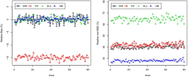
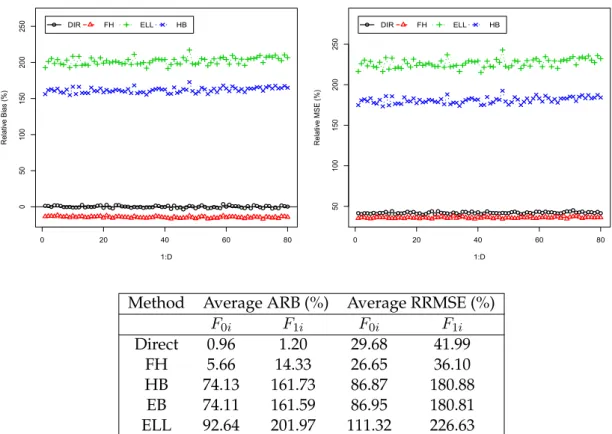
Figure2.1depicts the percent values of RB (left) and RRMSE (right) of the estimators of the domain poverty gaps F1i for each domain i. EB and Census EB estimates are
not shown in these plots because they are both practically equal to HB estimates and are plotted separately in Figure 2.2. Figure 2.1 left shows that direct, ELL and HB estimators are practically unbiased. In contrast, FH estimators display a substantial negative bias. Concerning efficiency, Figure 2.1 right shows that HB estimators have the smallest RRMSE whereas ELL estimators are the ones with the largest RRMSE. Conclusions for the poverty incidenceF0iare very similar.
Table2.1displays averages across domains of ARB and RRMSE of all the estimators, for both poverty incidence and poverty gap. We see that FH estimator exhibits a large ARB (over 6% for poverty incidence and close to 15% for poverty gap), whereas EB, HB and Census HB estimators have a very small ARB (< 1%). The latter estimators also achieve the smallest RRMSEs (slightly over 20% for poverty incidence and over 25% for
poverty gap). The largest RRMSE is obtained by ELL estimator (over 58%). Note that both ARB and RRMSE increase when estimating the poverty gap, because the poverty gap depends to a greater extent on the extreme of the left tail of the income distribution, which is more difficult to estimate correctly from a (finite) sample.
These results indicate that HB estimators are practically unbiased and clearly the most efficient among the considered estimators when the nested error model holds and the sample is drawn with srswor within each domain. The bias of FH estimators is due to the fact that they are attaching most of the weight to the regression-synthetic component, which relies exactly on the model, but here dataYij are generated from the
unit level model (2.9) and the domain means of the covariates X¯q,i = Ni−1 PNi
j=1xq,ij
are not linearly related with the poverty indicators Fαi. Thus, FH model fails due to
non-linearity of the poverty indicatorsFαi in the domain level covariatesX¯q,i,k= 1,2,
even if the unit level model holds exactly, because of the non-linearity ofFαias function
ofYij.
Figure 2.1:Percent RB (left) and RRMSE (right) of direct, FH, HB and ELL estimators of poverty gapF1i for each domainiunder the nested error model with srswor.
0 20 40 60 80 −15 −10 −5 0 5 Area Relativ e Bias (%) DIR FH ELL HB 0 20 40 60 80 30 40 50 60 70 80 Area Relativ e root MSE (%) DIR FH ELL HB
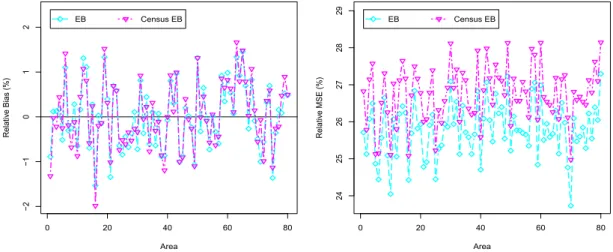
Figure 2.2 depicts percent RB (left) and RRMSE (right) of EB and Census EB estimates of the poverty gapF1ifor each domaini. This figure shows the great similarity
of EB and Census EB estimates ofF1i, even if sampling fractions in this simulation study
are not so small (ni/Ni = 1/5,i= 1, . . . , m).
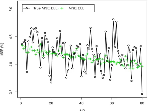
Next, we study ELL estimator of the MSE ofFˆαiELLgiven in (2.10). Figure2.3depicts the true model MSE of ELL estimators of the poverty gapF1i, labeled “True MSE ELL”
and the means across 10,000 simulations of ELL estimates of the MSE, MSEm( ˆFαiELL),
labeled “MSE ELL”, for each domain i. This figure shows that ELL estimates of the model MSE do not really track the true model MSEs for each domain even if we have
Method Average ARB (%) Average RRMSE (%) F0i F1i F0i F1i Direct 0.99 1.26 28.53 36.33 FH 6.34 14.78 26.26 38.16 HB 0.48 0.65 20.15 25.43 EB 0.51 0.67 20.41 25.75 Census EB 0.55 0.69 21.15 26.71 ELL 1.31 1.69 47.39 58.63
Table 2.1: Averages across domains of percent ARB and RRMSE for direct, FH, HB, EB, Census EB and ELL estimators of poverty incidenceF0iand poverty gapF1i, under the nested error model with srswor.
Figure 2.2: Percent RB (left) and RRMSE (right) of EB and Census EB estimators of poverty gapF1ifor each domainiunder the nested error model with srswor.
0 20 40 60 80 −2 −1 0 1 2 Area Relativ e Bias (%) EB Census EB 0 20 40 60 80 24 25 26 27 28 29 Area Relativ e MSE (%) EB Census EB
considered here random effects for the domains in the model (i.e., sampling clusters equal to domains). In the case that clusters are different from the domains, if we consider the original ELL method that includes only cluster effects but area effects are significant, then ELL estimates might seriously underestimate the MSE.
For the EB estimator, the parametric bootstrap procedure proposed byMolina and Rao(2010) approximates the true MSE reasonably well, seeMolina and Rao(2010). For HB estimator, posterior variance, approximated by Monte Carlo, is taken as measure of uncertainty.
2.3.2 Nested error model with informative sampling
We consider the same setup as in the previous simulation study, with the same popula-tion sizes, model parameters, auxiliary variables and poverty line. The only difference is that, in this simulation study, samples are drawn with informative sampling. When
Figure 2.3:True MSE of ELL estimators of poverty gapF1iand mean across simulations of ELL estimator of the MSE for each domaini, under the nested error model with srswor.
0 20 40 60 80 3.5 4.0 4.5 5.0 1:D MSE (%)
True MSE ELL MSE ELL
the sampling is informative, the probability of a sample depends on the values of the population vector y. Thus, under this setup, the simulations need to be performed with respect to the joint distribution of(y, s); that is, in each Monte Carlo replicatek, we draw a population vector y(k) and, given y(k), we draw a samples(k). A total of
K = 1,000population vectors y(k), k = 1, . . . , K, are generated from the true nested error model (2.9). Again, we consider that the target variables areEij = exp(Yij). The
samples(k)is drawn by Poisson sampling, with inclusion probabilities πij depending
on a random variable Zij that is correlated with the unexplained part ofYij, that is,
the model errorseij. Thus, for each population unitj from domaini, we generate a
Bernoulli random valueQij ∼Bern(πij), withπij =b−1exp(−aZij), wherea >0,b >0
andZij ∼ Gamma(τij, θij). To choose the values ofτij andθij, we consider two cases:
low and high level of informativeness. In the first case, we take τij = 5(3 + 0.1eij)
and θij = 0.25(3 + 0.1eij), which yield random values Zij with a 20% correlation
with the model errors eij. In the second case, we take τij = 5(4.5 + 1.5eij) and
θij = 0.25(4.5 + 1.5eij), yieldingZij with a 80% correlation witheij, which represents a
high level of informativeness. Note that, under this set up, the sample size is random because each unit in the population comes to the sample depending on its random valueQij. To make this simulation study comparable with the one in previous section,