MODELLING OF GENOTYPE BY ENVIRONMENT INTERACTION AND PREDICTION OF COMPLEX TRAITS ACROSS MULTIPLE ENVIRONMENTS AS A SYNTHESIS OF CROP GROWTH MODELLING, GENETICS AND STATISTICS
Thesis committee
Promotor
Prof. Dr F.A. van Eeuwijk Professor of Applied Statistics Wageningen University & Research
Co-promotor Dr M. Malosetti
Researcher, Applied Statistics Wageningen University & Research
Other members
Prof. Dr L.F.M Marcelis, Wageningen University & Research Dr C.D. Messina, DuPont Pioneer, Johnston, USA
Prof. Dr C.C. Schön, Technical University of Munich, Germany Prof. Dr B.J. Zwaan, Wageningen University & Research
This research was conducted under the auspices of the Graduate School of Production Ecology and Resource Conservation (PE & RC)
Modelling of Genotype by Environment Interaction and
Prediction of Complex Traits across Multiple Environments as
a Synthesis of Crop Growth Modelling, Genetics and Statistics
Daniela Bustos-Korts
Thesis
submitted in fulfilment of the requirement for the degree of doctor at Wageningen University
by the authority of the Rector Magnificus, Prof. Dr A.P.J. Mol,
in the presence of the
Thesis Committee appointed by the Academic Board to be defended in public
on Wednesday 15 November 2017 at 4 p.m. in the Aula.
Daniela Bustos-Korts
Modelling of Genotype by Environment Interaction and Prediction of Complex Traits across Multiple Environments as a Synthesis of Crop Growth Modelling, Genetics and Statistics, 340 pages.
PhD thesis, Wageningen University, Wageningen, The Netherlands (2017)
With references, with summary in English
ISBN: 978-94-6343-669-4
v
Bustos-Korts, D. (2017). Modelling of Genotype by Environment Interaction and Prediction of Complex Traits across Multiple Environments as a Synthesis of Crop Growth Modelling, Genetics and Statistics. PhD thesis, Wageningen University, the Netherlands.
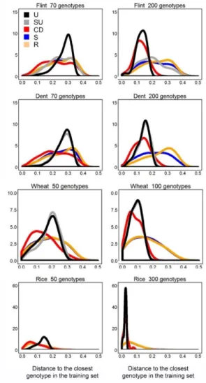
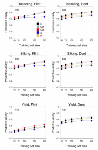
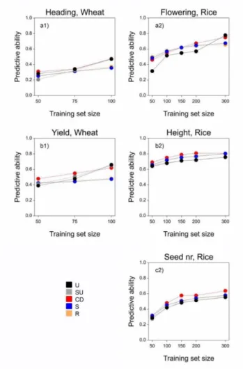
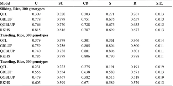
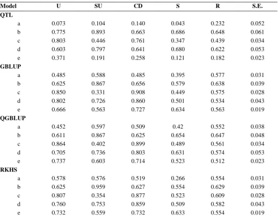
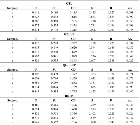
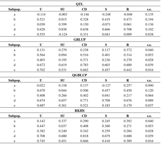
The main objective of plant breeders is to create and identify genotypes that are well-adapted to the target population of environments (TPE). The TPE corresponds to the future growing conditions in which the varieties produced by a breeding program will be grown. All possible genotypes that could be considered as selection candidates for a specific TPE are said to belong to the target population of genotypes, TPG. Genotypes commonly show different sensitivities to environmental gradients and then genotype by environment interaction (GxE) is observed. GxE can lead to changes in genotypic ranking, complicating the breeding process. The main aim of this thesis was to investigate statistical models and the combination of statistical and crop growth models to improve phenotype prediction across multiple environments. One aspect that determines the quality of phenotype prediction is the set of genotypes used to train the prediction model, especially when the TPG is structured. We proposed a method that uniformly covers the genetic space of the TPG, leading to a larger prediction accuracy than random sampling. We produced positive results for wheat, maize and rice. A second aspect that influences the accuracy of phenotype predictions is the choice of environments used to train the prediction model, which should capture the heterogeneity in the TPE. When accounting for heterogeneity in environmental quality, it is important to distinguish between repeatable and well predictable elements in the environmental conditions from those that are badly predictable. We proposed statistical methods based on the AMMI model and on mixed models to identify groups of environments that show repeatable GxE, illustrating our ideas with multi-environment wheat data in North-Western Europe. The importance of training set construction strategies and multi-environment genomic prediction models was also demonstrated for barley data. If breeders are interested in identifying the genetic basis of the target traits, it is advantageous to have a higher SNP density. In this thesis, we used exome sequence data of the EU-Whealbi-barley germplasm, which corresponds to a unique set of genotypes with a diverse origin, growth habit and breeding history.
vi
show that the EU-Whealbi-barley collection possesses a large diversity of promising alleles regulating the four traits we analysed. The last major topic addressed in this thesis is the use of a combination of statistical-genetic models and crop growth models (APSIM) as a strategy to assess the traits and phenotyping schemes to improve the prediction accuracy of a target trait like yield. We assess the potential of the combined modelling approach to characterize a sample of the TPG and TPE, and illustrate how trait correlations are modified by environmental conditions and by the genetic architecture of the sample of the TPE. We discuss the topics mentioned above, from a didactical perspective, proposing a list of subjects that should be covered in a GxE course for plant breeders. Finally, we discuss challenges and opportunities presented by the characterization of the TPE and TPG when using simulations based on statistical and crop growth models.
vii
Abstract v
Chapter 1 General Introduction 1
Chapter 2 Modelling of Genotype by Environment Interaction and Prediction of Complex Traits across Multiple
Environments as a Synthesis of Crop Growth Modelling, Genetics and Statistics
11
Chapter 3 Improvement of predictive ability by uniform coverage of the target genetic space
35
Chapter 4 Identifying regions in multi-environment trials by bilinear and mixed models: a case study of yield in wheat for North-Western Europe
75
Chapter 5 Predicting responses in multiple environments: issues in relation to genotype by environment interactions
101
Chapter 6 Modelling the genetic basis of adaptation and stability of the EU-WHEALBI-barley collection using exome capture and common garden experiments in contrasting environments
123
Chapter 7 A protocol combining statistical and crop growth modelling to evaluate phenotyping strategies useful for selection under different drought patterns
175
Chapter 8 What should students in plant breeding know about the statistical aspects of GxE?
219
Chapter 9 General Discussion 253
List of References 283
Summary 323
Curriculum Vitae 331
PE&RC Training and Education Statement 335
Acknowledgements 337
3 1.1.Introduction
The main goal of plant breeders is to create and identify genotypes that are well-adapted to the future growing conditions defined by the meteorological, soil and management at the growing area of interest (Cooper & Hammer, 1996). These growing conditions will influence the phenotypic response of individual genotypes. The functional form by which environmental inputs are translated into phenotypes is sometimes referred to as the reaction norm (Woltereck, 1909; Dobzhansky & Spassky, 1963; Sarkar, 1999; DeWitt & Scheiner, 2004). Reaction norms depend both on environmental inputs and genetic sensitivities to these environmental inputs. When the reaction norms for different genotypes are not parallel, this indicates the existence of genotype by environment interaction (GEI) (Finlay & Wilkinson, 1963; van Eeuwijk et al., 2005). An extreme form of GEI is cross-over interaction, where the ranking of the genotypes varies with the environmental conditions (Baker, 1988; Crossa et al., 2004). Cross-over interactions complicate the breeding process, making it necessary to recommend specific genotypes for specific environments.
Usually, GxE patterns are analysed for a set of environments that correspond to the future growing conditions of the genotypes created by the breeding programme. This set of environments is also referred to as ‘the target population of environments’, TPE (Comstock & Moll, 1963; Cooper & Hammer, 1996; Cooper et al., 2014). The TPE will influence the traits and adaptation mechanisms that are necessary for a genotype to perform well, showing a high yield. The traits that are relevant for adaptation to particular growing conditions influence the decision process of breeders, modifying the selection strategy applied within breeding programme. The selection strategy, together with the crossing scheme, shape the target population of genotypes (TPG), which corresponds to all possible genotypes that the breeding programme for the TPE hopes to develop during the coming years. The TPG coincides with the notion of selection candidates (Jannink et al., 2010; Schulz-Streeck et al. 2012; Albrecht et al. 2014).
To select well-adapted genotypes, predictions need to be made for the phenotype as a function of genotype and environment. These predictions can be made with statistical-genetic models, crop growth models or with a combination of statistical-genetic and crop growth
4
models. Statistical models to characterize GxE range from the conventional ANOVA to factorial regression type of models and mixed models integrating explicit environmental and physiological information (van Eeuwijk et al., 2005; Malosetti et al., 2013). Commonly used fixed models to characterize GxE are the Additive Main effects and Multiplicative Interactions (AMMI) and the Genotype main effects and Genotype by Environment interaction effects model (GGE) models (Gauch, 1992, 2013; Yan et al., 2000; Yan & Hunt, 2001). In fixed model terms, inferences are made with respect to the specific levels of genotypes and environments, whereas in random model terms, there is interest in the underlying distribution of the population (Searle et al., 2009). Both AMMI and GGE models allow examining GxE by means of biplots that provide a visual representation of which genotypes and environments are driving the interaction, allowing to group environments. To structure the network of testing sites, it is important to distinguish between GxE variation due to the consistent differences between locations, from the random year-to year variations (Atlin et al., 2000, 2011; Piepho & Möhring, 2005). If the phenotypic responses at particular locations have a certain degree of repeatability across years, these locations may be classified into ‘mega-environments’, which correspond to sets of environments of similar quality that show a reduced number of cross-over interactions (Rajaram et al., 1993; Gauch & Zobel, 1997). Within a mega-environment, similar genotypes can be recommended, simplifying the selection and the recommendation processes. Fixed-effects models to characterize GxE are certainly a useful tool for breeders, provided the GxE concerns well defined genotypes under repeatable environmental conditions. However, part of the GxE is commonly due to random trial-to-trial variations and not necessarily to repeatable GxE that would justify splitting the TPE in a number of mega-environments (Atlin et al., 2011). Random year-to-year variations can be handled by an adequate representation and replication of the testing sites across the TPE and by the use of mixed models that consider part of the GxE as a random process. Popular mixed models to characterize GxE are the unstructured model and the factor analytic model (Burgueño et al., 2008; Beeck et al., 2010). When the TPE can be subdivided into homogeneous mega-environments that show a consistent genotypic ranking across years, these mega-environments can also be either integrated into the mixed model as a fixed effect or used to model the variance-covariance structure. Modelling of the mega-environments explicitly allows to increase the response to selection and to obtain genotypes that are better
5
adapted to the within-mega-environment growing conditions (Atlin et al., 2000, 2011; Piepho & Möhring, 2005).
The availability of molecular markers allows identifying genomic regions underlying the phenotypic differences via QTL models. If the expected genetic similarity is homogeneous across the whole population, as in doubled haploid populations (DHs) or recombinant inbred lines (RILs), the significance of QTL effects is tested using a simple residual structure (Rebai et al., 1995; Lynch & Walsh, 1998). However, a more elaborate structure for the residual genetic variance is needed to model for multi-parent populations or diversity panels (Malosetti et al., 2007, 2011; Korte & Farlow, 2013; Garin et al., 2017). If the interest is not in detecting genomic regions associated with the trait, but in making phenotype predictions, it is in general convenient to move from QTL models to genomic prediction models. In genomic prediction models, no explicit significance threshold is used and all markers are used (Meuwissen et al., 2001). Genomic prediction models range from those accounting only for additive effects, like GBLUP (VanRaden, 2008), up to more elaborate models that allow for nonlinearities associated with non-additive genetic effects. A popular model allowing for non-additive effects is the reproducible Kernel Hilbert Spaces model (RKHS) (Gianola & van Kaam, 2008; de los Campos et al., 2009; Jiang & Reif, 2015). An alternative to mixed models for genomic prediction are the Bayesian models. There is a large number of Bayesian models for genomic prediction and they basically differ in the degree of shrinkage imposed on the markers genome-wide (Meuwissen et al., 2001; Hayes et al., 2009; Perez et al., 2010; Habier et al., 2011; de los Campos et al., 2013).
For a more explicit representation of the genotypic response across environments, it might be convenient to use factorial regression type of models with QTLs modulating the genotypic sensitivity to the environment. Examples for factorial regression-type of models can be seen in (Malosetti et al., 2004; Boer et al., 2007). More elaborate and dynamic characterization of the genotypic response to the environmental conditions can be modelled via functional mapping, which consists of a combination of QTLs and mathematical functions that model the QTL effects over time (Malosetti et al., 2006; Wu & Lin, 2006; van Eeuwijk et al., 2010; Li & Sillanpää, 2015). An increasingly popular approach to explicitly model the functional relationships between plant physiology and the environment is by using crop growth models
6
(Yin et al., 2000, 2005; Tardieu et al., 2005). Crop growth models usually decompose the target trait (grain yield) into a number of underlying genetically-correlated traits, called ‘intermediate traits’ (Yin et al., 2004), ‘indicator traits’ (Calus & Veerkamp, 2011), ‘secondary traits’ (Rutkoski et al., 2016) or ‘components’ (Porter & Gawith, 1999) that might have a simpler genetic basis and larger heritability than the target trait (Yin et al., 2004; Tardieu & Tuberosa, 2010; Cabrera-Bosquet et al., 2016). Examples of intermediate traits are biomass, grain number and grain weight. Intermediate traits are calculated indirectly from a set of environmental inputs and genotype-dependent parameters derived from prior experimentation. GxE in the target trait is then a consequence of the interactions between the intermediate phenotypes (Chapman et al., 2003; Tardieu et al., 2005; Chenu et al., 2009; Makumburage et al., 2013). GxE modelling via crop growth models is commonly done using a two-step approach; first, the genotype dependent parameters are estimated from experimental data, via QTL or genomic prediction models. Then, these predicted parameter values are introduced into the crop growth model to generate predictions for the target trait across multiple environments (Yin et al., 2000; Zheng et al., 2013). An alternative-two stage approach had been recently proposed by (Technow et al., 2015; Cooper et al., 2016), where component traits are treated as latent variables for prediction that arise from the propagation of the marker effects on yield through the crop growth model structure.
1.2.Objectives and outline of the thesis
The general objective of this thesis is to propose and evaluate models to characterize GxE and predict complex traits across multiple environments. To achieve this goal, we used statistical models and the crop growth model APSIM-Wheat. The first specific objective was to set the scene about prediction scenarios that are interesting for breeders and to discuss how either statistical models, crop growth models or the combination of both types of models can be used to predict phenotypes across environments (Chapter 2). The scenarios that we discussed in Chapter 2 correspond to the prediction of unobserved genotypes in observed environments, the prediction of observed genotypes in unobserved environments and finally, the prediction of unobserved genotypes in unobserved environments. The second specific objective of this thesis, assessed in Chapter 3, was to propose a strategy to construct the training set of genotypes, improving the prediction accuracy of unobserved genotypes in
7
observed environments. The main underlying hypothesis for our proposed training set construction method was that a homogeneous representation of the genetic diversity (genetic space) in the TPG leads to larger prediction accuracy. We compared our method based on uniform coverage of the genetic space, with commonly used methods like random sampling, stratified sampling and with a method that maximizes the generalized coefficient of determination, proposed by (Rincent et al., 2012).
When the goal is to make predictions in a multi-environment setting, the first task is to characterize the GxE patterns present in the TPE because this will influence the multi-environment prediction model that will have the largest accuracy. Therefore, the strategy to select candidates across a range of environments is highly dependent on the structure of GxE. This structure depends on the importance of year-to-year variability and on whether locations can be classified into more homogeneous groups, also called ‘mega-environments’. In Chapter 4, we assessed strategies based on the additive main effects and multiplicative interactions model (AMMI, Gauch, 1992, 2013; Gauch & Zobel, 1997)) as applied to repeatable genotype by location interaction and on mixed models to identify regions that are internally more homogeneous. We presented examples for historical multi-environment trials for wheat in Denmark, Germany, The Netherlands and the United Kingdom. In Chapter 5, we illustrate the concepts discussed in Chapters 2, 3 and 4, applying them to a multi-environment genomic prediction context. Issues as the similarity between training and prediction environments and the design of training-validation schemes are also discussed and illustrated in Chapter 5. In Chapter 6, we apply multi-environment mixed models to characterize the EU-Whealbi germplasm collection as a source of valuable alleles for adaptation to European environments. The EU-Whealbi collection corresponds to 511 barley genotypes with a very wide range of origins and breeding history. EU-Whealbi was genotypically characterized with exome sequence data and phenotypically characterized in six very diverse European environments. Thanks to the genome sequence data, we could explore the effects of haplotypes instead of single SNPs, adding an extra layer the complexity to the statistical analysis.
In Chapter 7, we switch from the prediction of single traits observed at a single time point to the modelling of multiple traits simultaneously to improve the prediction accuracy
8
of the target trait. We also compare strategies to model phenotypes of multiple time-points simultaneously to characterize trait dynamics during the growing season. For intermediate traits to be useful to improve the prediction accuracy of the target trait, they have to be correlated to the target trait and have a large heritability. Trait correlations depend on the environment and heritability depends on the experimental and measurement quality. In Chapter 7, we propose the combination of statistical-genetic models and the APSIM crop growth model as a tool to assess the potential of traits and phenotyping strategies to improve the prediction accuracy of the target trait. Many of the concepts and statistical models discussed in Chapters 2 to 7 are presented in Chapter 8 from an educational/didactical perspective. In this Chapter, we propose a schedule of topics that should be covered in a GxE course for plant breeders. We also provide an overview of the trends in the usage of different GxE models in the literature over time. Finally, in Chapter 9, we discuss the convenience of modelling approaches based on statistical models, crop growth models or a combination of statistical and crop growth modelling for different breeding situations. We also discuss how high throughput genotyping and high throughput phenotyping can be used to increase the chances of selecting better-adapted varieties and about technical considerations when combining statistical-genetic and crop growth models to assess breeding strategies.
Modelling of
Genotype by Environment Interaction and
Prediction of Complex Traits across
Multiple Environments as a Synthesis of
Crop Growth Modelling, Genetics and Statistics
Daniela Bustos-Korts1,2, Marcos Malosetti1, Scott Chapman3, Fred van Eeuwijk1*
1. Biometris, Wageningen University & Research Centre 2. C.T. de Wit Graduate School for Production Ecology & Resource Conservation (PE&RC) 3. CSIRO Plant Industry and Climate Adaptation Flagship
This Chapter is published as:
Bustos-Korts D, Malosetti M, Chapman S, van Eeuwijk FA (2016) Modelling of Genotype by Environment Interaction and Prediction of Complex Traits across Multiple Environments as a Synthesis of Crop Growth Modelling, Genetics and Statistics. In: Yin X, Struik PC (eds) Crop Systems Biology - Narrowing the Gaps between Crop Modelling and Genetics. Springer, pp 55–82
12 Abstract
Selection processes in plant breeding depend critically on the quality of phenotype predictions. The phenotype is classically predicted as a function of genotypic and environmental information. Models for phenotype prediction contain a mixture of statistical, genetic and physiological elements. In this chapter, we discuss prediction from linear mixed models (LMMs), with an emphasis on statistics, and prediction from crop growth models (CGMs), with an emphasis on physiology. Three modalities of prediction are distinguished: predictions for new genotypes under known environmental conditions, predictions for known genotypes under new environmental conditions, and predictions for new genotypes under new environmental conditions.
For LMMs, the genotypic input information includes molecular marker variation, while the environmental input can consist of meteorological, soil and management variables. However, integrated types of environmental characterizations obtained from crop growth models (CGMs) can also serve as environmental covariable in LMMs. LMMs consist of a fixed part, corresponding to the mean for a particular genotype in a particular environment and a random part defined by genotypic and environmental variances and correlations. For prediction via the fixed part, genotypic and/or environmental covariables are required as in classical regression. For predictions via the random part, correlations need to be estimated between observed and new genotypes, between observed and new environments, or both. These correlations can be based on similarities calculated from genotypic and environmental covariables. A simple type of covariable assigns genotypes to sub-populations and environments to regions. Such groupings can improve phenotype prediction.
For a second type of phenotype prediction, we consider crop growth models. CGMs predict a target phenotype as a non-linear function of underlying intermediate phenotypes. The intermediate phenotypes are outcomes of functions defined on genotype dependent CGM parameters and classical environmental descriptors. While the intermediate phenotypes may still show some genotype by environment interaction, the genotype dependent CGM parameters should be consistent across environmental conditions. The CGM parameters are regressed on molecular marker information to allow phenotype prediction from molecular marker information and standard physiologically relevant environmental information.
Both LMMs and CGMs require extensive characterization of genotypes and environments. High-throughput technologies for genotyping and phenotyping provide new opportunities for upscaling phenotype prediction and increasing the response to selection in the breeding process.
13 2.1. Introduction
The target production area for most arable crops spans a range of environmental conditions. In the absence of diseases and pests (not considered in this review), local environmental conditions are a function of meteorological and soil variables on the one hand and management interventions on the other hand. These conditions will influence the phenotypic response of individual genotypes, and to some extent genotypes will create their ‘own’ environment, e.g. depending on how they use soil water across the season. The functional form by which environmental inputs are translated into phenotypes is sometimes referred to as the reaction norm (Woltereck 1909; Dobzhansky and Spassky 1963; Sarkar 1999; DeWitt and Scheiner 2004). Reaction norms depend both on environmental inputs and genetic factors. For a given (multi-locus) genotype, the reaction norm is the functional relationship between the phenotype and an environmental gradient, and is often linearised in some way. Modelling of the reaction norms for a set of genotypes is a central objective in many breeding and genetic studies. The prediction of the phenotypic response as a function of genetic and environmental factors is the basis for decisions that involve selection of superior genotypes for a defined environmental range (Hammer et al. 2006; Chenu et al. 2011; Sadras et al. 2013).
Several important concepts in breeding and genetics have been defined in relation to the behaviour of reaction norms for a population of genotypes. Firstly, when the reaction norms are non-constant, genotypes are said to show ‘plasticity’ (Bradshaw et al. 1965; DeWitt and Scheiner 2004; Sadras and Lawson 2011). Secondly, when the reaction norms for different genotypes are not parallel, this indicates the existence of genotype by environment interaction (GEI) (Finlay and Wilkinson 1963; van Eeuwijk et al. 2005). An extreme form of GEI is cross-over interaction, where the ranking of the genotypes varies with the environmental conditions (Baker 1988; Muir et al. 1992; Crossa et al. 2004). Another important concept in the context of the comparison of reaction norms is adaptation (Wright 1931, 1932; Finlay and Wilkinson 1963; Romagosa and Fox 1993; Cooper and Hammer 1996; Cooper 1999; Romagosa et al. 2013), i.e., some genotypes do better than other ones in a defined set of environmental conditions, the reaction norms of the adapted genotypes are then always above those of the less adapted. Finally, for a given genotype, ‘stability’ measures quantify the variation around the reaction norm (Lin and Binns 1988; Piepho 1998). So, while plasticity, GEI and adaptation refer to the expected response curve, which may be most simply thought of as the expectation in a linear regression model, stability refers to the variation around this expected response at a defined set of environmental conditions (Slafer and Kernich 1996; DeWitt and Scheiner 2004; van Eeuwijk et al. 2005; van Eeuwijk et al. 2010).
14
To select genotypes with superior average performance or a given degree of adaptation, predictions need to be made for the phenotype as a function of genotype and environment. These types of predictions occur at various stages in a breeding programme. In the early stages of breeding programmes, seed is limiting and large numbers of new genotypes produced as offspring from crosses between well-chosen parents are evaluated in one or a few trials, normally in small plots. For the earliest stages of a breeding programme, modelling of reaction norms is not possible and selection takes place on the mean performance. At intermediate stages, offspring populations are tested in a limited number of trials at various locations for one or a few years. In those cases when seed is still limiting, it is attractive to use partially replicated designs (Cullis et al. 2006; Smith et al. 2006) so that genotypes can be tested at a larger sample of environmental conditions. Selection can be done on the mean across trials, but there are also possibilities to select for adaptation. At the later stages, when there is sufficient seed for individual genotypes, a limited number of genotypes can be tested in a large number of trials, with again possibilities for selection on wide adaptation to a wide set of environments or narrow adaptation to a limited set of environments (Cooper et al. 2014). Simultaneously, at this stage selection on stability is possible.
When a population of genotypes is evaluated in multiple trials, reaction norms can be fitted to help in describing the observed data efficiently and to allow some form of selection on properties of the reaction norm. To evaluate the predictive quality of reaction norm models, special cross validation (CV) schemes have been proposed. In CV schemes, the data are subdivided in a training set, used to estimate model parameters, and a test set, used to assess the correlation between predicted values and observed values. Such a correlation is termed prediction ‘accuracy’ (Meuwissen et al. 2001). For multiple environment data, various CV strategies have been proposed (Crossa et al. 2010; Burgueño et al. 2012; Heslot et al. 2012; Zhao et al. 2012; Heslot et al. 2013; Crossa et al. 2014). At this point, it is useful to clarify some nomenclature. When genotypes were tested, evaluated or observed in at least one environment, we indicate this by the letter G. When this was not the case we use nG. For environments the same rule can be defined: E for observed environments, with at least one observed genotype, and nE for environments without observations. Specific combinations of genotype and environment can have been observed, GE, or not, nGE. Following this terminology, the set [G, E, GE] would indicate a genotype that was observed and an environment that was observed, while also the specific combination of genotype and environment was observed. The combination [G, E, nGE] indicates a genotype and environment that have been observed, but the specific combination of genotype and environment was not observed. This latter situation is typical for unbalanced genotype by environment data.
15
Figure 1 shows four scenarios that are relevant to prediction of phenotypes from genotypes and environments as well as to the calculation of accuracies and CV strategies. Scheme 1 pertains to situations in which both genotypes and environments were observed. Specific combinations of genotypes and environments may be present, [G, E, GE] or absent [G, E, nGE]. Phenotype predictions for Scheme 1 can be made by simple additive models. The Schemes 2, 3 and 4 are more interesting and we will concentrate on those. Potential strategies for assessment of accuracy in genomic prediction are predictions for new genotypes in observed environments [nG, E, nGE] (Scheme 2, Fig. 1); predictions for observed genotypes in new environments [G, nE, nGE] (Scheme 3, Fig. 1); and predictions for new genotypes in new environments [nG, nE, nGE] (Scheme 4, Fig. 1) (Utz et al. 2000; Calus and Veerkamp 2011; Burgueño et al. 2012; Schulz-Streeck et al. 2012; Guo et al. 2013; Crossa et al. 2014). Scheme 4 of CV obviously represents the strictest type of accuracy assessment. (For the notation, whenever nG or nE appears, necessarily nGE needs to appear as well, so for Schemes 2, 3 and 4, we can omit the specification nGE.)
Figure 1. Prediction scenarios, depending on whether genotypes were observed (G) or not observed (nG), and on whether environments were observed (E) or not observed (nE).
16
To produce phenotype predictions for new genotypes (nG) from observed genotypes (G), it is essential to use statistical models that allow us to connect the new genotypes to the observed genotypes. The connections between nG and G can be achieved by the inclusion of explicit genotypic covariables in the statistical model, and/or by borrowing information via the correlation structure among genotypes, defined by their genetic similarities. Analogously, for predicting new environments, there needs to be a connection between nE and E via explicit environmental covariables and/or the correlation structure among environments. The latter correlation structure is an expression of environmental similarity as estimated from environmental characterizations.
In this chapter, we introduce linear mixed models (LMMs) as our default class of statistical prediction models. LMMs can be described as consisting of two parts: 1) a fixed part, corresponding to the mean; and 2) a random part defined by variances and covariances. Predictions in LMMs can be obtained via the fixed and the random part, although the statistical mechanism for prediction in those two cases is different. As an illustration, we provide an LMM for the phenotype of genotype i in environment j: 𝑦𝑦𝑖𝑖𝑗𝑗= 𝜇𝜇𝑗𝑗+ 𝑥𝑥𝑖𝑖𝛼𝛼𝑗𝑗+ 𝛽𝛽𝑖𝑖𝑧𝑧𝑗𝑗+ 𝐺𝐺𝐺𝐺𝑖𝑖𝑗𝑗+ 𝑒𝑒𝑖𝑖𝑗𝑗 (van Eeuwijk et al. 2010). The fixed part of this model is given by the expectation,
or mean, for genotype i in environment j: 𝜇𝜇𝑖𝑖𝑗𝑗= 𝜇𝜇𝑗𝑗+ 𝑥𝑥𝑖𝑖𝛼𝛼𝑗𝑗+ 𝛽𝛽𝑖𝑖𝑧𝑧𝑗𝑗. Here 𝜇𝜇𝑗𝑗 is a fixed intercept (mean) for environment j, 𝑥𝑥𝑖𝑖 is a genotypic covariable, for example a molecular marker, 𝛼𝛼𝑗𝑗 is an environment specific slope corresponding to 𝑥𝑥𝑖𝑖. When 𝑥𝑥𝑖𝑖 is a molecular marker, 𝛼𝛼𝑗𝑗 is an environment specific quantitative trait locus (QTL) effect (Malosetti et al. 2004; Boer et al. 2007). For the environments, 𝑧𝑧𝑗𝑗 is an environmental covariable, for example, a drought stress index, and 𝛽𝛽𝑖𝑖 is a corresponding genotype specific slope, for example a genotype-specific sensitivity to drought stress.
For prediction via the fixed part, we use genotypic and/or environmental covariables as in classical regression (van Eeuwijk et al. 1996). Besides values for the covariable, 𝑥𝑥𝑖𝑖 and 𝑧𝑧𝑗𝑗, prediction requires that we have estimates for the slopes, 𝛼𝛼𝑗𝑗 and 𝛽𝛽𝑖𝑖. These can be obtained by fitting a model for the mean to training data, where we need to select suitable genotypic and/or environmental covariables. For prediction, we combine the estimated slopes in the training set with the values for genotypic and/or environmental covariables in the test set.
The random part of the model is determined by the terms 𝐺𝐺𝐺𝐺𝑖𝑖𝑗𝑗 and 𝑒𝑒𝑖𝑖𝑗𝑗, the first term representing the (residual) genotypic effect of genotype i in environment j, the second term containing experimental (block) and measurement errors. (Random terms in model formulations are underlined.) The random terms are assumed to have a Gaussian distribution, with expectation zero and proper variance-covariance structures. The important random term for prediction purposes is 𝐺𝐺𝐺𝐺𝑖𝑖𝑗𝑗. For this term, the correlations among genotypes on the one
17
hand and the correlations among environments on the other hand determine the predictive properties of the LMM. Thus, for predictions via the random part of the LMM, correlations need to be estimated between observed and new genotypes (Scheme 2), observed and new environments (Scheme 3), or both (Scheme 4). Correlations among genotypes can be estimated from genotypic covariables, including molecular markers, and pedigree data, or a combination of genotypic covariables and pedigree. Correlations among environments follow from environmental covariables. Although important, we will largely ignore the error term 𝑒𝑒𝑖𝑖𝑗𝑗 in the remainder of this chapter. See Smith et al. (2001a) and Smith et al. (2005) for discussion on models for 𝑒𝑒𝑖𝑖𝑗𝑗.
The realization of the predictive potential of LMMs depends on the selection of genotypic covariables and environmental covariables, for the fixed part as well as for the random part. Physiological knowledge on genotypes and environments can help in the choice of covariables for inclusion in LMMs. For example, knowledge on the structure and use of crop growth models (CGMs) can help in the dissection of complex traits (Chapman et al. 2002b; Edmeades et al. 2004; Reynolds et al. 2009a), thereby suggesting genotypic and environmental covariables for inclusion in predictive LMMs. A CGM can suggest writing a complex target trait as a function of a set of simpler component traits and a set of environmental input variables (Yin et al. 2003, 2004; Chenu et al. 2008; Hammer et al. 2010). These component traits are traditionally related to physiologically parameters in CGMs. The CGM produces GEI as an emerging property of the interaction between the physiological parameters and the environmental information (Chapman et al. 2002a, 2008; Hammer et al. 2002, 2006, 2010). Interpreting the CGM as a function that transforms physiological parameters and environmental inputs into a complex trait, we can understand that when the CGM can be approximated by a linear function, the component traits may be entered as genotypic covariables and the environmental inputs as environmental covariables in an LMM for the complex trait.
In Section 2, we will discuss how statistical LMM models can be used to predict phenotypic responses for new genotypes in observed environments (Scheme 2; [nG, E, nGE]), observed genotypes in unobserved (new) environments (Scheme 3; [G, nE, nGE]), or new genotypes in new environments (Scheme 4; [nG, nE, nGE]). In Section 3, we will discuss the use of CGMs to predict the performance of genotypes for environments in which they were not tested. Section 4 will discuss the contribution of high throughput genotyping and phenotyping to models for phenotype prediction. Strategies to group genotypes and environments will also be discussed in this section. We finish with some concluding remarks in Section 5.
18
2.2. Statistical models to predict phenotypic performance
Section 2.1 presents statistical models for predicting the phenotype of genotypes that were so far not tested in the environments for which we want to predict, although we do have information about these environments from phenotypic evaluations for other genotypes [nG, E, nGE], Scheme 2 in Fig. 1. The connection between observed genotypes (G) and not observed genotypes (nG) will come from explicit genotypic covariables and/or the genetic correlations among genotypes. Section 2.2 describes statistical models for predicting phenotypes in environments that were not used to test genotypes, although we do have phenotypic information about these genotypes in other environments [G, nE, nGE], Scheme 3 in Fig. 1. The connection between observed environments (E) and unobserved environment (nE), will result from the inclusion of explicit environmental covariables and/or the correlations among environments calculated on the basis of environmental characterizations. Section 2.3 discusses the most challenging prediction scenarios; predicting the phenotype of genotypes that were not tested so far, for environments that neither were tested [nG, nE, nGE], Scheme 4 in Fig. 1. Here, both explicit genotypic and environmental covariables are required for prediction.
2.2.1. Statistical models to predict performance of unobserved genotypes in observed environments [nG, E, nGE]
Quantitative traits are determined by many loci, with allelic effects varying in magnitude. Specific genomic regions significantly associated with phenotypic variation may be identified as quantitative trait loci, or QTLs (see Chapter 1 of this book by Baldazzi et al.). Besides QTLs, or instead thereof, many other loci with small additive effects (polygenic effects) can contribute to phenotypic variation. None of these loci with small effects might by itself have an important phenotypic effect, but these loci together can still make a sizeable contribution to the phenotype. Our first model, Model 1, includes loci with relatively large quantitative effects (QTLs) together with loci that have small effects.
𝑦𝑦𝑖𝑖𝑗𝑗𝑡𝑡 = 𝜇𝜇𝑗𝑗+ ∑𝑄𝑄𝑖𝑖=1𝑥𝑥𝑖𝑖𝑖𝑖𝛼𝛼𝑗𝑗𝑖𝑖 + 𝐺𝐺𝑖𝑖𝑗𝑗+ 𝑒𝑒𝑖𝑖𝑗𝑗 (1)
In the multi-environment Model 1, 𝑦𝑦𝑖𝑖𝑗𝑗𝑡𝑡 represents the target trait, t, (for example, yield) of genotype i in environment j, 𝜇𝜇𝑗𝑗is a fixed intercept term for each environment, 𝑥𝑥𝑖𝑖𝑖𝑖 is a genotypic covariable that represents DNA information of genotype i at QTL position q, and 𝛼𝛼𝑗𝑗𝑖𝑖 is the additive effect of the fixed QTL q in environment j.𝐺𝐺𝑖𝑖𝑗𝑗 represents the residual
genetic effect (polygenic effects) for genotype i in environment j. The matrix with elements 𝐺𝐺𝑖𝑖𝑗𝑗, {𝐺𝐺𝑖𝑖𝑗𝑗}, has a multivariate normal distribution with zero mean, 𝟎𝟎, and, as we will see later,
19
a highly structured variance-covariance matrix 𝜮𝜮; {𝐺𝐺𝑖𝑖𝑗𝑗}~𝑀𝑀𝑀𝑀𝑀𝑀(𝟎𝟎, 𝜮𝜮). (For notational simplicity, we will omit the dimensions of the various matrices.) 𝜮𝜮 defines the genetic variances and covariance for any two pair of observations, 𝑦𝑦𝑖𝑖𝑗𝑗𝑡𝑡 and 𝑦𝑦 𝑖𝑖𝑡𝑡´𝑗𝑗´ and depends on the
genetic and environmental similarities of the two genotypes, i and i’, and the two environments j and j’. The term 𝑒𝑒𝑖𝑖𝑗𝑗 stands for a non-genetic residual, {𝑒𝑒𝑖𝑖𝑗𝑗}~𝑀𝑀𝑀𝑀𝑀𝑀(𝟎𝟎, 𝑹𝑹), with 𝑹𝑹 often allowing for specific residual variances per environment.
A simplification of Model 1 omits the genetic residual, 𝐺𝐺𝑖𝑖𝑗𝑗, and is appropriate when QTLs account for all of the genetic variation:
𝑦𝑦𝑖𝑖𝑗𝑗𝑡𝑡 = 𝜇𝜇 + ∑𝑄𝑄𝑖𝑖=1𝑥𝑥𝑖𝑖𝑖𝑖𝛼𝛼𝑗𝑗𝑖𝑖 + 𝑒𝑒𝑖𝑖𝑗𝑗 (1.1)
When Model 1.1 fits the data well, the performance of the unobserved genotype i in environment j can be predicted as;
𝑦𝑦�𝑖𝑖𝑗𝑗𝑡𝑡 = 𝜇𝜇̂𝑗𝑗+ � 𝑥𝑥𝑖𝑖𝑖𝑖𝛼𝛼�𝑗𝑗𝑖𝑖 𝑄𝑄
𝑖𝑖=1
Compared with single-environment QTL models, multi-environment QTL models like Model 1 or Model 1.1 are more powerful in picking up QTLs and generally explain a larger amount of the genetic variance (Piepho 2000; Piepho and Möhring 2005; Mathews et al. 2008; Alimi et al. 2013). It has been shown that jointly considering multivariate phenotypes (i.e., the phenotype in multiple environments) allows a substantially greater separation between genotype classes than when considering univariate phenotypes (i.e., phenotype in a single environment) (Stephens 2013).
Another simplification of Model 1 occurs when we assume that there are no large discrete genetic effects in the form of QTLs that drive phenotypic differences, but that genetic effects are exclusively of a polygenic nature. A prediction model that generalizes the single environment genomic best linear unbiased prediction (G-BLUP) approach of (Meuwissen et al. 2001) to multi-environment prediction can be defined as:
𝑦𝑦𝑖𝑖𝑗𝑗𝑡𝑡 = 𝜇𝜇𝑗𝑗+ 𝐺𝐺𝑖𝑖𝑗𝑗+ 𝑒𝑒𝑖𝑖𝑗𝑗 (1.2)
In Model 1.2, the distribution of the polygenic effects 𝐺𝐺𝑖𝑖𝑗𝑗 is {𝐺𝐺𝑖𝑖𝑗𝑗}~𝑀𝑀𝑀𝑀𝑀𝑀(𝟎𝟎, 𝜮𝜮). Since 𝜮𝜮 is a function of the genetic and environment similarities, the larger the similarity of unobserved genotypes with observed genotypes, and the larger the similarity of observed environments with unobserved environments, the more information is available for phenotype prediction,
20
and the higher is the prediction accuracy (Crossa et al. 2006; Albrecht et al. 2014). Analogous to the classical partitioning of genetic and environmental effects, the covariance matrix 𝜮𝜮 can be partitioned into a ‘genotypic’ variance-covariance matrix (𝜮𝜮𝐺𝐺), and an ‘environmental’ variance-covariance matrix (𝜮𝜮𝐸𝐸), such that 𝜮𝜮 = 𝜮𝜮𝑮𝑮⨂𝜮𝜮𝐸𝐸, i.e., the Kronecker product of the genotypic variance-covariance matrix and the environmental variance-covariance matrix (West et al. 2006; Smith et al. 2005). It is important to realize that although 𝜮𝜮𝐸𝐸 is called an ‘environmental’ variance-covariance matrix, 𝜮𝜮𝐸𝐸 reflects genetic correlations among environments, and so plays a role in forming predictions in the multi-environment context. Examples of commonly used models for these two covariance matrices are given below.
𝜮𝜮𝐺𝐺can be modelled as 𝜮𝜮𝐺𝐺= 𝑨𝑨, where 𝑨𝑨 corresponds to the expected additive relationship
matrix calculated from the coefficients of coancestry estimated from the pedigree, or to the realized additive relationship matrix estimated from molecular markers (Piepho et al. 2008). If the one step prediction with statistical models uses pedigree information, 𝐺𝐺𝑖𝑖𝑗𝑗 is commonly called “breeding value” (Falconer and Mackay 1996; Piepho et al. 2008). On the other hand, if the prediction uses molecular marker information, it is called “genomic estimated breeding value” (Burgueño et al. 2012; Piepho 2009).
In the multi-environment context, genotypic variances tend to change across environments with consequent changes in genotypic correlations for pairs of these environments. A flexible variance-covariance structure across environments 𝜮𝜮𝐸𝐸, is required to achieve higher prediction accuracies. One flexible and parsimonious model for variances and covariances/correlations across environments is the factor analytic model (FA) (Table 1) (Smith et al. 2001a, 2005; Mathews et al. 2008).
The decision about when it is convenient to use Models 1, 1.1, or 1.2 depends on the genetic architecture of the target trait. If the trait is regulated by a few QTLs with large effects, a QTL model (Model 1.1) might provide the largest prediction accuracy. On the other hand, traits like grain yield, which are regulated by many genes with small effects might not show any significant QTL that can be included in Model 1.1. In this case, Model 1.2, whose predictions we will call GE-BLUPs because they can account for GEI, should integrate the large number of small additive effects into a multi-environment prediction model. For the intermediate case when traits have a few QTLs with large effects, and many other loci with very small additive effects, Model 1 is adequate. Bernardo (2014) suggested that it is convenient to consider QTLs (or genes) as fixed effects when they account for more than 10% of the genetic variance. The simulations made by Bernardo (2014) show that the most adequate model depends on the genetic architecture of the trait, i.e., on the number of QTLs and the magnitudes of the QTL effects.
21
Table 1. Variance-covariance models for the environmental covariance (𝛴𝛴𝐸𝐸), ordered by increasing number of parameters. For simplicity, these examples assume three environments (m=3).
Name Number of parameters Structure Identity 1 �𝜎𝜎 2 0 0 0 𝜎𝜎2 0 0 0 𝜎𝜎2� Compound symmetry 2 �𝜎𝜎 2+ 𝜑𝜑 𝜑𝜑 𝜑𝜑 𝜑𝜑 𝜎𝜎2+ 𝜑𝜑 𝜑𝜑 𝜑𝜑 𝜑𝜑 𝜎𝜎2+ 𝜑𝜑�
Factor analytic, order 1 2m
�𝜆𝜆1 2+ 𝜓𝜓 1 𝜆𝜆1𝜆𝜆2 𝜆𝜆1𝜆𝜆3 𝜆𝜆2𝜆𝜆1 𝜆𝜆22+ 𝜓𝜓2 𝜆𝜆2𝜆𝜆3 𝜆𝜆3𝜆𝜆1 𝜆𝜆3𝜆𝜆2 𝜆𝜆32+ 𝜓𝜓3 � Unstructured m(m+1)/2 � 𝜎𝜎12 𝜎𝜎12 𝜎𝜎13 𝜎𝜎21 𝜎𝜎22 𝜎𝜎23 𝜎𝜎31 𝜎𝜎32 𝜎𝜎32 �
2.2.2. Statistical models to predict performance of observed genotypes in new environments
After genotypes have been phenotyped in some environments, it can be useful to predict their performance in other environments that were not used for evaluation. New environments could, for example, include future trials at known locations, which implies that none of the genotypes were observed in that environment yet [G, nE, nGE]. Thus, the correlation between observed environments and the predicted environments cannot be estimated from phenotypic data, or direct observations on the complex trait. In this case, we may use environmental covariables, like meteorological, soil or management covariables, as predictors in models for the mean or define correlations between environments in models for the variance-covariance structure.
Models for the mean that can be used to predict phenotypes in unobserved environments usually correspond to factorial regression models that incorporate environmental covariables.
22
These models explicitly estimate the sensitivity of the QTL to environmental covariables (Model 2) (Campbell et al. 2004; Boer et al. 2007; Laperche et al. 2007; Malosetti et al. 2013; Romagosa et al. 2013). Hence, model parameters can have biological interpretation.
𝑦𝑦𝑖𝑖𝑗𝑗= 𝜇𝜇𝑗𝑗+ ∑𝑄𝑄𝑖𝑖=1𝑥𝑥𝑖𝑖𝑖𝑖�𝛾𝛾𝑖𝑖+ 𝛿𝛿𝑖𝑖𝑧𝑧𝑗𝑗� + 𝐺𝐺𝑖𝑖𝑗𝑗+ 𝑒𝑒𝑖𝑖𝑗𝑗 (2)
In Model 2, the additive effects (𝛼𝛼𝑗𝑗𝑖𝑖) of the fixed QTL q in environment j of Model 1are replaced by a regression formulation, �𝛾𝛾𝑖𝑖+ 𝛿𝛿𝑖𝑖𝑧𝑧𝑗𝑗�, in which the effect of QTL q is a function of the environmental covariable 𝑧𝑧𝑗𝑗, and so changes over environments. When the covariable 𝑧𝑧𝑗𝑗 is centered, the intercept term, 𝛾𝛾𝑖𝑖, corresponds to the effect of the QTL in the average
environment, while the slope 𝛿𝛿𝑖𝑖 corresponds to the sensitivity of the QTL q to the environmental covariable 𝑧𝑧𝑗𝑗. Although Model 2 does not explicitly restrict the environmental covariables to a particular range, it should be considered that crops respond differently to covariables in the environmental extremes (e.g., too cold or too warm). So, the sensitivity of the genotype to the environmental covariables cannot be assumed constant outside the range of environments in which 𝛿𝛿𝑖𝑖 was estimated. A second issue that needs to be taken into account is that models like Model 2 do not make explicit in which phenological stage the environmental covariable is considered. Since the sensitivity of a crop to the environment varies throughout the development, environmental covariables included in the prediction model need to coincide with the developmental timing used to estimate the sensitivity.
For example, Boer et al. (2007) analysed grain yield and grain moisture for F5 maize testcross progenies evaluated across 12 environments in the U.S. corn belt. Since QTLs did not have a constant effect across environments (QTL by environment interaction), QTL effects were modelled conditional on longitude and year, both consequences of temperature differences during critical stages of the development. This factorial regression model allows prediction of yield and moisture at any location provided that temperatures during specific developmental stages are contained within those of the observed environments.
A second example is shown by Malosetti et al. (2004), who identified QTLs conferring differential sensitivity of grain yield to temperature during heading in a double haploid barley population. In a model like Model 2, the average daily temperature range during heading was the most important environmental covariable explaining differential QTL expression, i.e., the QTL allele from the parental line Steptoe, conferred an extra grain yield of 0.112 ton ha-1 for
each extra degree Celsius during heading. Hence, yield could be predicted for unobserved environments if the average temperature for such environments was available. In that sense, Model 2 is closer to CGM than Model 1 because Model 2 explicitly represents environments on a continuous scale.
23
The second way to use environmental information for prediction is using environmental covariables to estimate similarities (covariances) among environments, analogous to the way molecular markers are used to characterize similarity among genotypes. If environmental covariables are considered as an indicator of environmental similarity, they can be used to estimate the environmental variance-covariance matrix in Model 1.2. Hence, 𝜮𝜮𝐸𝐸= 𝜴𝜴, where 𝜴𝜴 is the variance-covariance matrix that accounts for the similarity in environmental conditions. The larger the covariance between observed and unobserved environments, the more information can be shared to make the predictions. The genotypic covariance 𝜮𝜮𝐺𝐺 can be modelled as explained in Section 2.1 by imposing an additive relationship matrix to define 𝜮𝜮𝐺𝐺= 𝑨𝑨, where 𝑨𝑨 can be estimated from the pedigree and/or from molecular markers.
Using multiple climatic variables to model the environmental covariance, as proposed by Jarquín et al. (2013) shows promise as a tool to predict genotypic performance in unobserved environments. However, many environmental covariables are correlated and not all need to be included in the model. Mechanistic CGMs such as APSIM have shown to be a good integrative tool to select subsets of variables that characterize environmental similarity (Chapman 2008).
2.2.3. Statistical models to predict performance of unobserved genotypes in new environments
Section 2.1 presented models that used genotypic covariables to predict the phenotype on unobserved genotypes. Section 2.2 described how environmental covariables can be used in factorial regression models for prediction, and how to estimate the environmental covariance of a random term, necessary for prediction along the random part of an LMM. This Section 2.3 will combine both situations, aiming to predict the phenotype of genotypes that have not been tested yet for environments that have not been used for evaluation.
When predicting unobserved genotypes in new environments, both genotypic and environmental covariables are needed. In factorial regression-type of models, prediction of unobserved genotypes is possible, provided that the additive effects of each QTL-allele can be estimated from the tested genotypes. The phenotypes of unobserved genotypes can also be predicted in new environments, provided that the sensitivity of the QTL effects along an environmental gradient (e.g., temperature), can be estimated from observed environments. In the example of Malosetti et al. (2004) presented in Section 2.2, phenotype prediction is possible for any environment provided the temperature remains within the range used to estimate the QTL sensitivity to temperature.
24
In models that entirely rely on the use of the variance-covariance structures imposed on genotypes and environments, prediction of unobserved genotypes in new environments is possible via the reconstruction of the full covariance matrix 𝜮𝜮 from its components, 𝜮𝜮𝐺𝐺 and 𝜮𝜮𝐸𝐸. For the genotypic part this runs via explicit pedigree information or information from
genotypic covariables (molecular markers), while for the environmental part correlations between environments can be estimated from environmental characterization (temperature, precipitation, soil characteristics, etc.). Note that while in Section 2.1, 𝜮𝜮𝐺𝐺 was calculated from genotypic covariables, and 𝜮𝜮𝐸𝐸 was estimated from the phenotypic data on the target trait, here both 𝜮𝜮𝐺𝐺and 𝜮𝜮𝐸𝐸 are estimated from explicit covariables.
2.3. Crop growth models to predict genotypic performance
The algorithms in a CGM predict the target trait (e.g., grain yield) as a non-linear combination of underlying intermediate phenotypes (also commonly called “components”, e.g., biomass), which are calculated indirectly from a set of inputs to the CGM that typically comprise environment (soil, weather, and nutrients) data and CGM parameters derived from prior experimentation. GEI in the target trait is then a consequence of the interactions between the intermediate phenotypes (Chapman et al. 2003; Tardieu 2003; Tardieu et al. 2005; Chenu et al. 2009; Makumburage et al. 2013).
Considering the CGM in reverse, we can state that the value of the target trait is able to be ‘dissected’ into these intermediate phenotypes (See Chapter 7 of this book by Hammer et al.). Although these intermediate phenotypes are likely to show less GEI than the target trait, they still correspond to an integration of genotypic responses to environmental conditions (e.g., they may show GEI). Ideally, a complete dissection of the target trait would comprise of a set of CGM input parameters that depend only on the genotype (for example, a genotypic sensitivity of development rate to the air temperature), and to environmental covariables (Model 2), i.e., CGM parameters that do not show GEI (Slafer 2003; Yin et al. 2003; Bertin et al. 2010; Alam et al. 2014). The target trait for genotype i in environment j can be written as a function of CGM parameters and environmental inputs as follows:
𝑦𝑦𝑖𝑖𝑗𝑗𝑡𝑡 = ∫ 𝑓𝑓 �𝒚𝒚𝑖𝑖𝑃𝑃; 𝒛𝒛𝑗𝑗� 𝑑𝑑𝑑𝑑 + 𝑒𝑒𝑖𝑖 (3)
In Model 3, 𝑦𝑦𝑖𝑖𝑗𝑗𝑡𝑡 represents the target trait for genotype i in environment j, which is modelled as a function of multiple CGM parameters 𝒚𝒚𝑖𝑖𝑃𝑃 (p for parameter in superscript) and multiple environmental inputs, 𝒛𝒛𝑗𝑗 integrated over time (Fig. 2). The function f ( ; ) embodies the algorithms that transform CGM parameters into intermediate phenotypes as well as the interactions between the intermediate phenotypes that lead to the target trait.
25
A commonly-studied CGM is APSIM, which currently has modules for several crops, e.g., wheat, canola, sorghum (Keating et al. 2003; Holzworth et al. 2014). In the case of APSIM-Wheat, growth (biomass accumulation) and development (phenological events, the functionality of plant structures or appearance of new structures) are calculated on a daily basis (Wang et al. 2002). The final phenotype (e.g., grain yield) is calculated as a function of a series of intermediate phenotypes. Examples of intermediate phenotypes are biomass, radiation use efficiency and radiation interception on any given day or accumulated to a given day (Fig. 2). Intermediate phenotypes depend on CGM parameters that are genetically determined, and which modulate the phenotypic response to environmental covariables. An example of CGM parameters is the development rate to flowering in wheat where the parameters are vernalization requirement and sensitivity to photoperiod, which are regulated by the VRN and the PPD alleles, and regulate the phenotypic response (phenology) to temperature and photoperiod (Zheng et al. 2013).
CGM parameters, 𝒚𝒚𝑖𝑖𝑃𝑃, for phenotyped genotypes can be directly observed, estimated or calculated from the phenotypic measurements. However, given that CGM parameters depend on the genotype, they can also be predicted from genotypic covariables, i.e., molecular marker information. When we can identify the genetic basis of physiological parameters in terms of underlying QTLs, or, equivalently, when we can predict the physiological parameters from marker information, we can effectively predict the target trait from marker information and environmental inputs provided the intermediate traits and their interactions have been correctly identified and implemented in the CGM. Hence, predicted CGM parameters enable to predict the phenotype of genotypes that have not been observed yet. The prediction for individual CGM parameters (𝑦𝑦𝑖𝑖𝑃𝑃) would look like Model 4:
𝑦𝑦𝑖𝑖𝑃𝑃= 𝜇𝜇 + ∑𝑄𝑄𝑖𝑖=1𝑥𝑥𝑖𝑖𝑖𝑖𝛼𝛼𝑖𝑖 + 𝐺𝐺𝑖𝑖+ 𝑒𝑒𝑖𝑖 (4)
Like Model 1, Model 4 can be modified to include (i) only the QTLs, in a QTL model (Model 4.1) or (ii) only the polygenic effects (𝐺𝐺𝑖𝑖), in a genomic prediction model with the random effects 𝐺𝐺𝑖𝑖 being structured by a genetic relationship matrix (Model 4.2).
𝑦𝑦𝑖𝑖𝑃𝑃 = 𝜇𝜇 + ∑𝑄𝑄𝑖𝑖=1𝑥𝑥𝑖𝑖𝑖𝑖𝛼𝛼𝑖𝑖 + 𝑒𝑒𝑖𝑖 (4.1)
𝑦𝑦𝑖𝑖𝑃𝑃= 𝜇𝜇 + 𝐺𝐺𝑖𝑖+ 𝑒𝑒𝑖𝑖 (4.2)
If more than one CGM parameter is to be predicted from molecular markers and/or pedigree information, Models 4, 4.1, and 4.2 could also be expanded to a multi-trait prediction model that takes into account possible correlations among the CGM parameters,
26
in a model that is similar to the multi-environment Model 1. Modelling traits simultaneously allows to gain power for QTL detection and to detect QTLs with pleiotropic effects (Alimi et al. 2013; Stephens 2013).
Figure 2. Representation of the main parameters of wheat yield used in the APSIM-CGM. Grey boxes correspond to intermediate phenotypes that are determined by the genotype and the environment (i.e. they show potentially large GEI), black boxes correspond to CGM parameters that are dependent on the genotype, and white boxes represent environmental covariables (http://www.apsim.info/).
Predictions for multiple CGM parameters, 𝒚𝒚�𝑖𝑖𝑃𝑃, can be used as input in Model 3 to calculate intermediate phenotypes, and produce the prediction for the target trait, 𝜇𝜇̂𝑖𝑖𝑗𝑗𝑡𝑡, in Model 5.
27
In Model 5, the prediction accuracy of the target trait depends on the accuracy of the prediction of each of the components, and on the ability of the functions that transform CGM parameters into intermediate phenotypes to correctly describe the processes leading to the target trait.
CGMs with known/predicted genotypic parameters are a potentially useful tool to understand which traits can be advantageous in a given environment, and also to identify management practices that contribute to improved crop productivity (Yin et al. 2004; Hammer et al. 2006; Reynolds et al. 2009b; Harrison et al. 2014). In the context of adaptation to climate change, Zheng et al. (2012) modelled how phenology of current wheat varieties would influence their adaptation to future environments, which are expected to show different CO2 and precipitation levels. In their second paper, Zheng et al. (2013)
demonstrated that the flowering time of spring wheat genotypes can be modelled using the composition of their VRN1 and Ppd-D1 alleles together with responses derived from a single experiment with four environments: +/- treatments for vernalisation and extended photoperiod. Allelic combinations of loci Vrn-A1, Vrn-B1, Vrn-D1, and Ppd-D1 were used to predict APSIM-wheat parameters of a population of genotypes. From a single experiment (replicated in two years), they validated the model with more than 250 wheat genotypes across the entire Australian wheat belt, and were able to simulate flowering time for any weather records in the wheat belt. These conclusions can be useful to guide breeders in the process of determining which alleles should be considered in the selection process.
Bogard et al. (2014) extended this approach further to model the drivers of flowering time in winter wheat as functions of major genes as well as SNPs derived from association mapping, i.e., allowing prediction of unknown genotypes (but with known genes and SNPs) in new environments. In both Zheng et al. (2013) and Bogard et al. (2014), the predictions for heading date using the gene-based predicted parameters corresponded well with the observed dates to heading. Attributes that contributed to a successful phenotype prediction were (i) a well-defined CGM for heading date (Slafer and Rawson 1994), (ii) a well-defined set of environmental covariables with corresponding CGM parameters, and (iii) a well understood genetic basis of the CGM parameters (Snape et al. 2001).
The same approach has also shown to be successful for other more complex and less heritable traits such as grain yield under drought. For example, Chenu et al. (2009) used APSIM to model the impact of QTLs controlling the intermediate traits leaf and silk elongation on maize grain yield. The intercept and slope of these intermediate traits in response to meristem temperature, evaporative demand and soil water deficit were genotype-dependent (Reymond et al. 2003; Reymond et al. 2004).
28
Unfortunately, the identification of CGM parameters is sometimes less straightforward for complex traits like grain yield. Yin et al. (2000) showed an example in barley with a successful estimation of QTL effects for the CGM parameters, but with a poor prediction of grain yield. The correlation between the observed CGM parameters, i.e. phenotype of CGM parameters, and the QTL-predictions of the same parameters was high. However, the correlation between yield predictions of the CGM, whether phenotype based or QTL prediction based, and observed yield was not high. The cause of the poor predictions did not reside in the fact that the CGM parameters were replaced by predicted parameters from the QTL model, but in the fact that the CGM was unable to predict yield from its component traits. Similar work has been recently reported by Gu et al. (2014) on grain yield of rice crop, using a new CGM, which gave more promising results. However, efforts to improve CGM for predicting complex traits like grain yield are still strongly needed.
The example from Yin et al. (2000) shows that although the integrated statistical and CGM modelling allows for a larger flexibility, it might result in more complex and fragile models, because the approach can break down at the level of the estimation of the CGM parameters and at the level of the integration of these CGM parameters to calculate the intermediate phenotypes. However, even if the CGM are not fully able to predict the target trait, it is valuable to develop models of intermediate traits as well as for yield per se. Breeders can still be interested to recombine lines with high levels of proven intermediate traits with the expectation that these should on average result in better yield when further crossing and selection is done, i.e., because the selection on intermediate traits should already have improved part of the physiological adaptation pathway (Cooper et al. 2014). If breeders select mainly on yield per se, then it may be less likely that selections will also have high radiation use efficiency (RUE) or transpiration efficiency (TE) or traits for which genetic variation was not expressed in the given selection environment.
The examples of Zheng et al. (2013), Bogard et al. (2014), and Chenu et al. (2009) show that CGMs are a tool to integrate complex information from the genotypic, organ, and crop level. Dissection of a target trait into component traits at different levels of biological organisation allows phenotype prediction for the target trait in the face of genotype by environment and QTL by environment interactions for that same trait. Hence, the combined approach of statistical QTL-modelling and CGM is an alternative to model complex GEI interactions (Yin et al. 2004).
29 2.4. Further considerations
2.4.1. Classification of environments
Sections 2.2 and 2.3 presented models to predict the performance of genotypes in new environments ([G, nE, nGE] or [nG, nE, nGE]). However, if there are repeatable patterns that allow to classify environments, these patterns might help to reduce the complexity of 𝜮𝜮𝐸𝐸 and thereby improve the accuracy of prediction.
One example of repeatable patterns that often justifies to group environments is the presence of regions. Here, we understand ‘regions’ (or mega-environments) as a group of locations where genotypes perform consistently across years (Bull et al. 1992; Gauch and Zobel 1997; Basford and Cooper 1998; Yan et al. 2000). Environments inside the same region are expected to be more homogeneous in terms of genotypic ranking, i.e., less GEI inside the regions (e.g. Atlin et al. 2000; Burgueño et al. 2008). In dryland production areas, other groupings may relate to characteristics of the soil (shallow/deep, low/high water holding capacity) and the management of the crop (sowing date, row spacing arrangement, etc.). De la Vega and Chapman (2010) showed how multiple component traits related to yield for a complex set of mega-environments in Argentina.
If locations can be grouped into regions, it is generally convenient to breed for specific adaptation to those regions, instead of broad adaptation across regions (Atlin et al. 2000, 2011). In this case, predictions can be produced for the whole of a region, or for new environments within a region. Precision of yield estimates might still benefit from the information of neighbouring regions by means of the covariance structure in a mixed model (Piepho and Möhring 2005; Kleinknecht et al. 2013).
When phenotypes are not available for all the locations of interest, environmental covariables can also be used to classify environments, and reduce the complexity of 𝜮𝜮𝐸𝐸. Classifying environments into regions on the basis of environmental similarity, potentially allows to (i) predict new environments (as discussed in Sections 2.2 and 2.3, and also (ii) define the target population of environments, where a particular genotype is to be evaluated (Chapman et al. 2000a; Hammer et al. 2002; Chenu et al. 2011). CGMs are a powerful tool to identify relevant environmental factors (Chapman 2008; Messina et al. 2011), and the periods when the crop is most sensitive to those factors (Chenu et al. 2013). For example, considering drought seasonal patterns could give a better indication of the environment types, instead of the total rainfall per year (Chapman et al. 2000a, 2000b).