A Survey on Automatic Parameter Tuning for Big Data Processing Systems

43

Processing Systems

HERODOTOS HERODOTOU,

YUXING CHEN and JIAHENG LU,

Big data processing systems (e.g., Hadoop, Spark, Storm) contain a vast number of configuration parame-ters controlling parallelism, I/O behavior, memory settings, and compression. Improper parameter settings can cause significant performance degradation and stability issues. However, regular users and even expert administrators grapple with understanding and tuning them to achieve good performance. We investigate ex-isting approaches on parameter tuning for both batch and stream data processing systems and classify them into six categories: rule-based, cost modeling, simulation-based, experiment-driven, machine learning, and adaptive tuning. We summarize the pros and cons of each approach and raise some open research problems for automatic parameter tuning.

CCS Concepts: •Computer systems organization→Self-organizing autonomic computing; • Infor-mation systems→Computing platforms;

Additional Key Words and Phrases: Parameter tuning, self-tuning, MapReduce, Spark, Storm, stream ACM Reference format:

Herodotos Herodotou, Yuxing Chen, and Jiaheng Lu. 2020. A Survey on Automatic Parameter Tuning for Big Data Processing Systems.ACM Comput. Surv.53, 2, Article 43 (April 2020), 37 pages.

https://doi.org/10.1145/3381027

1 INTRODUCTION

The continuous growth of the World Wide Web, E-commerce, Internet of Things (IoT), and other applications is generating massive amounts of ever-increasing raw data every day [88]. Large-scale data analytics platforms, including both batch data processing systems (e.g., Hadoop MapReduce [4], Spark [6]), as well as stream data processing systems (e.g., Apache Storm [11], Heron [75], Flink [3], Samza [5]), have emerged to assist with the Big Data challenge, i.e., to efficiently col-lect, process, and analyze massive volumes of heterogeneous data. Achieving good and robust system performance at such a scale is the foundation for successfully performing timely and cost-effective analytics (either offline or in real-time). However, system performance is directly linked to a vast array of configuration parameters, which control various aspects of system execu-tion, ranging from low-level memory settings and thread counts to higher-level decisions such as

Jiaheng Lu and Yuxing Chen are partially supported by Finnish Academy Project 310321.

Authors’ addresses: H. Herodotou, Cyprus University of Technology, 30 Arch. Kyprianos Str., Limassol, 3036, Cyprus; email: [email protected]; Y. Chen, University of Helsinki, C215, Exactum, Kumpula, Gustaf Hallstromin katu 2b, Helsinki, Finland; email: [email protected]; J. Lu, University of Helsinki, C212, Exactum, Kumpula, Gustaf Hall-stromin katu 2b, Helsinki, Finland; email: [email protected].

Permission to make digital or hard copies of part or all of this work for personal or classroom use is granted without fee provided that copies are not made or distributed for profit or commercial advantage and that copies bear this notice and the full citation on the first page. Copyrights for third-party components of this work must be honored. For all other uses, contact the owner/author(s).

© 2020 Copyright held by the owner/author(s). 0360-0300/2020/04-ART43

resource management and load balancing [88]. Improper settings of configuration parameters are shown to have detrimental effects on the overall system performance and stability [39,61,103].

The use of automated parameter tuning techniques is a promising, yet challenging approach for optimizing system performance. The major challenges are:

(1) Large and complex parameter space:Hadoop, Spark, and Storm have over 200 con-figurable parameters each [22,70,103]. To make matters worse, some parameters might affect the performance of different jobs in different ways, while certain groups of param-eters may have dependent effects (i.e., a good setting for one parameter may depend on the setting of a different parameter) [61,66].

(2) System scale and complexity: As data analytics platforms have grown in scale and complexity, system administrators may need to configure and tune hundreds to thousands of nodes, some equipped with different CPUs, memory, storage media, and network stacks [80]. In addition, executing MapReduce or Spark workloads with iterative stages and tasks in parallel or serial makes it challenging to observe and model workload performance [46]. (3) Lack of input data statistics:Data statistics are almost never available for MapReduce and Spark applications, since data often reside in semi- or un-structured files and are opaque until accessed [58]. As for stream applications, the input data are a real-time data stream that typically experiences significant variations in workload properties [34]. Classification of Approaches:A considerable amount of past research tackles the problem of performance optimization by partially or fully automating the process of finding near-optimal parameter values for executing jobs in big data processing systems. This survey performs a com-prehensive study of existing parameter-tuning approaches, which address various challenges to-wards high throughput and resource utilization, fast response time, and cost-effectiveness. Due to the various challenges and scenarios addressed, different strategies or approaches are proposed accordingly. We classify these approaches into the following six categories:

(1) Rule-basedapproaches assist users with tuning some system parameters based on the experience of human experts, online tutorials, or tuning instructions. They usually require no models or log information and are suitable for quickly bootstrapping the system. (2) Cost modelingapproaches build efficient performance prediction models by using

an-alytical (white-box) cost functions developed based on a deep understanding of system internals. A few experimental logs and some input statistics are typically required to es-tablish the model.

(3) Simulation-basedapproaches build performance prediction models based on modular or complete system simulation, enabling users to simulate an execution under different parameter settings or cluster resources.

(4) Experiment-drivenapproaches execute an application, i.e., an experiment, repeatedly with different parameter settings, guided by a search algorithm and the feedback provided by the logs of the actual runs.

(5) Machine learning approaches establish performance prediction models by employing machine learning methods. They typically consider the complex system as a whole and assume no (or limited) knowledge of system internals (i.e., they treat the system as a black box).

(6) Adaptiveapproaches tune configuration parameters adaptively while an application is running, i.e., they can adjust the parameter settings as the environment changes based on a variety of methods. They enable tuning of ad hoc and long-running applications.

Table 1. Feature Comparison among the Six Parameter Tuning Approaches

Feature Rule-based Cost modeling Simulation Experiment-driven Machine learning Adaptive Key modeling technique rules cost functions simulation search algorithms ML models mixed

# of parameters modeled few some some many many some

System understanding strong strong strong light no strong Need for history logs no light light strong strong light Need for data input stats no light light no strong light

Real tests to run no some no yes yes yes

Time to build model efficient efficient medium slow slow medium

# of metrics predicted few few some few many some

Prediction accuracy low medium medium medium high medium

Adapt to workload adaptive light light no no adaptive

Adapt to system changes no no light no adaptive light

Table1summarizes and compares the various key features and functionalities provided by the six approaches in terms of modeling (e.g., technique, number of parameter models, system under-standing), need for statistics or runs, prediction accuracy, and adaptability to workload and system changes. It is worth noting that by addressing the number of parameters, system understanding, and need for data input statistics, we summarize the approaches’ pertinence concerning the three aforementioned challenges. The six approaches will be analyzed in-depth and compared within the context of both batch and stream data processing systems in the following sections. While most approaches fit neatly into one of the aforementioned categories, some approaches may use techniques that span more than one. For example, Starfish [58,61] builds detailed cost models for modeling the MapReduce execution process and uses a small simulator component for simulating the task scheduling decisions. In such cases, we categorize the approach based on the predominant technique. Thus, we classify Starfish as a cost modeling approach.

Main Contributions:This manuscript reviews the representative techniques of parameter tuning on big data analytics systems. The comprehensive nature of this survey helps to motivate new parameter-tuning techniques, to develop real-world tuning applications, as well as to serve as a technical reference for selecting and comparing the existing tuning strategies. Particularly, the key contributions of this survey are:

(1) We introduce the area of parameter tuning and provide a general classification of the relevant approaches.

(2) We discuss parameter tuning from various perspectives for two different classes of sys-tems; namely, batch and stream processing systems.

(3) We describe in detail the key features for existing representative tuning methods. (4) We describe open research problems and showcase that parameter tuning forms a

chal-lenging research area, where solutions can be exploited in a variety of real-world use cases.

Related Work:Several existing surveys deal with the performance optimization and/or efficient resource management of large-scale data processing systems. Babu et al. [16] covered the core fea-tures of several analytics platforms (e.g., Hadoop, Spark, Dryad), including resource management, task scheduling, and query optimization. In terms of parameter tuning, it briefly discussed only the Starfish line of work [58,61], elaborated in Section4.1. Two existing surveys [38,77] on MapReduce discuss how previous approaches address several of the weaknesses and limitations of MapReduce, including high communication cost, inflexible access to input data, redundant processing, as well as lack of iterations, interactive processing, and support for n-way operations. However, the issue

of configuration parameter tuning is not addressed in either survey. Hirzel et al. [63] present a list of optimizations for stream processing, such as task placement and load balancing. The only relevant optimization discussed is tuning the batching size, which is only one of the many pa-rameters that can impact performance in a streaming setting. Dayarathna et al. [34] focus on the system architecture and use cases of stream processing platforms and only briefly discuss per-formance scalability. A more recent survey [99] proposes a classification for parallelization and elasticity methods in stream processing systems but lacks any discussion on automatic parameter tuning. Autonomic computing brings together the work of computer science and control commu-nities with the purpose of developing autonomic systems, i.e., systems that can manage themselves automatically. An excellent survey [65] lists the key applications of autonomic computing and dis-cusses the related approaches. Automatic parameter tuning shares a similar aim with autonomic computing in that it improves the big data systems by decreasing human involvement in the pa-rameter configuration process. However, the framework and methods in autonomic computing are quite different from those surveyed here. To the best of our knowledge, no other manuscript exists that deals with parameter tuning to an extent and depth comparable to this survey. Outline:The remaining manuscript is organized as follows: Section2presents background infor-mation on the execution and the configuration parameters of popular batch and stream processing systems. Sections3–8offer a detailed description of parameter tuning approaches organized into the aforementioned six categories. Section9concludes the survey while discussing challenges and open research problems.

2 PRELIMINARIES

Existing large-scale data processing systems can be categorized intobatchandstream process-ing systems. In the batch model, data are typically collected and stored before beprocess-ing fed into an analytics platform such as Hadoop MapReduce or Spark. In the stream model, however, data ar-rive continuously and are processed immediately by a streaming platform such as Apache Storm, Flink, or Spark Streaming. In both cases, the execution behavior and performance of the system are controlled by dozens of configuration parameters. Sections2.1and2.2present the system architec-ture in conjunction with important parameters for popular batch and stream processing systems, respectively. Finally, Section2.3formalizes the problem of automatic parameter tuning.

2.1 Batch Processing Systems

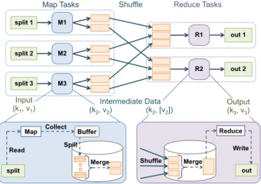
In this survey, we focus on Hadoop MapReduce [4] and Apache Spark [6], the two most popular platforms for big data analytics.MapReduceis both a programming model and an execution engine for massive data analysis [35]. As a programming model, MapReduce consists of themap(k1,v1) and the reduce (k2,list(v2)) user-defined functions. For every input key-valuepair k1,v1, the map(k1,v1)function is used to output zero or more intermediate key-value pairsk2,v2, as shown in Figure1. The intermediate valuesv2are grouped together according to the key valuesk2 to generate the pairsk2,list(v2). Next, thereduce (k2,list(v2)) function is invoked for each such pair and produces zero or more output key-value pairsk3,v3. The keys (k1–k3) and the values (v1–v3) could be of any data type.

A Hadoop MapReduce job executes as a set of parallel map and reduce tasks on a compute cluster (see Figure1). Each map task processes one input split, which is a portion of the input dataset to be processed by the job, and generates a portion of the intermediate data. After map tasks complete, Hadoop uses an external sort-merge algorithm to group all intermediate key-value pairs andshuffles(i.e., transfers) them to the cluster nodes that will run the reduce tasks. Finally, the intermediate data will be processed by the reduce tasks, which will generate the final results of the job [123]. The map and reduce tasks can be further decomposed intophases,as shown in

Fig. 1. Execution of a MapReduce job as a set of map and reduce tasks. The map task execution is further decomposed into “read,” “map,” “collect,” “spill,” and “merge” phases. The reduce task execution is further decomposed into “shuffle,” “merge,” “reduce,” and “write” phases [58].

Figure1. The map task execution is composed of five phases: (a)“read”for reading the data input from the distributed file system; (b)“map”for executing the user-defined map function; (c)“collect” for buffering and partitioning map outputs; (d)“spill”for sorting, combining, and writing map outputs to local disk; and (e)“merge”for merging sorted spill files. The reduce task execution is composed of four phases: (a)“shuffle”for copying map output data to the reduce node; (b)“merge” for merging sorted map outputs; (c)“reduce”for executing the user-defined reduce function; and (d)“write”for writing the final output to the distributed file system [58].

In the early versions of Hadoop (up to v1.2.1; 2014), map and reduce tasks were running in a predefined number of map and reduceslotsper cluster node. However, a MapReduce job typically requires many map slots when it starts, while it needs to reduce slots after the map tasks complete [16]. Hence, the static allocation of resources into map and reduce slots often leads to lowered cluster utilization. In the next versions, namedApache YARN[111], Hadoop created two separate functional layers: one for allocating resources to running applications and one for managing the application’s life-cycle. The resource allocation model in YARN introduced the notion ofresource containers, which describe node resources such as CPU and memory. In this model, applications can ask for different container specifications at different points of their execution, giving rise to interesting research problems on how to determine the appropriate amounts of resources for each task as well as how to allocate resources among them [16]. Several follow-up works developed extended resource allocation and scheduling mechanisms for geographically distributed big data processing frameworks based on Hadoop MapReduce and Spark [37].

The Hadoop configuration parameters (in both versions) impact several aspects of job execu-tion at the different phases, such as task concurrency, memory allocaexecu-tion, I/O performance, and network bandwidth usage. Currently, Hadoop has over 200 parameters, from which about 30 can have a substantial effect on job performance [16]. Table2lists some of the most influential configu-ration parameters (valid up to Hadoop v3.2.1), which are used in optimizing Hadoop performance. Default parameter values are either provided by Hadoop or are specified by a system administrator and are used unless the user explicitly specifies parameter values during job submission.

An early comparative study between Hadoop and two parallel database systems revealed that Hadoop was slower by a factor of 3.1 to 6.5 in processing several data-intensive analytical

Table 2. Key Performance-aware Configuration Parameters for Hadoop [48]

Parameter Name Parameter Description Default

“dfs.block.size” The default block size for files stored on HDFS 128 MB

“mapreduce.job.maps” Number of map tasks 2

“mapreduce.job.reduces” Number of reduce tasks 1

“mapreduce.combine.class” A combine function for preaggregating map outputs before the shuffle phase null “mapreduce.map.combine.

minspills”

Min number of map output spill files present for using the combine function 3 “mapreduce.map.output.

compress”

Flag for enabling compression of map output data FALSE “mapreduce.map.sort.spill.

percent”

Percent of “mapreduce.task.io.sort.mb” buffer to fill before spilling the map output to local disk

0.8 “mapreduce.output.

fileoutputformat.compress”

Flag for enabling compression of job output data FALSE “mapreduce.reduce.input.

buffer.percent”

Percent of reducer’s memory devoted to buffering map output data while executing the reduce task

0 “mapreduce.reduce.merge.

inmem.threshold”

Max number of shuffled map output pairs before initiating merging during the shuffle

1000 “mapreduce.reduce.shuffle.

input.buffer.percent”

Percent of reducer’s memory devoted to buffering map output data during the shuffle

0.7 “mapreduce.reduce.shuffle.

merge.percent”

Percent of reduce task’s memory to fill before initiating merging during the shuffle

0.66 “mapreduce.reduce.shuffle.

parallelcopies”

Max number of parallel threads that transfer data from map tasks to a reduce task

5 “mapreduce.task.io.sort.factor” Max number of data streams to merge during external sorting 10 “mapreduce.task.io.sort.mb” Size of memory buffer that stores the map output data 100MB “mapreduce.tasktracker.map.

tasks.maximum”

Max number of map tasks executed concurrently at a cluster node (number of map slots)

2 “mapreduce.tasktracker.reduce.

tasks.maximum”

Max number of reduce tasks executed concurrently at a cluster node (number of reduce slots)

2

workloads [94]. Motivated by these results, two performance studies [15,68] conducted in-depth analyses of Hadoop to find the most critical factors and configuration parameters that affect its performance. Both studies concluded that by meticulously tuning these factors and parameters, the performance of Hadoop could be dramatically improved and be more comparable to the per-formance of parallel database systems.

A follow-up study [126] performed Principal Component Analysis (PCA) to determine the Hadoop configuration parameters that significantly affect system performance, yielding three principal components. The first one is composed of configuration settings that directly affect the I/O performance of MapReduce jobs:io.sort.factorand parameters for compressing map and final output. The second component contains settings that control the memory size used to buffer intermediate data (i.e., JVM memory and buffer sizes for intermediate data stored in map and re-duce tasks). The final component reflects the parallelism in the MapRere-duce job and contains the number of tasks and data copiers during the shuffle.

Apache Spark[6] is an open-source distributed framework that simplifies the development of applications that execute in parallel on computing clusters in a fault-tolerant way. Its interface is based on the notion of theRDD(“Resilient Distributed Dataset”), which is a multiset of objects with a read-only property spread over a cluster and maintained in a fault-tolerant way [132]. As a programming abstraction, an RDD represents a multiset of objects that can be split through a high-performance computing cluster. Operations on RDDs are also divided and executed in

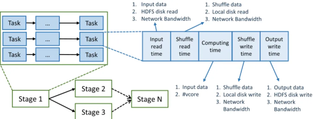
Fig. 2. A Spark job execution consists of multiple parallel or sequential stages and each stage is composed of multiple tasks. The performance of each task is influenced by several factors at each task phase [46,103].

parallel across the cluster, leading to fast and scalable parallel processing. The overall architec-ture is composed of the Spark Core and a set of libraries, presented next.

Spark Core:Spark Core is the fundamental framework, providing task distribution, scheduling, as well as basic I/O functionalities. It also exposes an application programming interface (API) for the RDD data objects. The interface involves several operations (e.g.,map,filter,reduce) on RDDs by calling a function on Spark in a developer-friendly fashion, concealing the complexity of distributed processing. Figure2presents the execution of a Spark job decomposed into stages and tasks [46,103]. In a specific task, the overall computation time consists of procedures for input read, shuffle read, computing, shuffle write, and output write times. The computation time for each of these procedures may be affected by different factors. For example, computing time may be affected by the input data size and the number of assigned CPU cores.

Spark Libraries:Spark’s popularity as a big data analytics platform has grown mainly due to its mature libraries, which are widely used in academia and industry. The four main libraries are:

(1) Spark SQL[14], which supports standard SQL connectivity as well as a standard interface for reading from and writing to other data stores including HDFS, Apache Hive, Apache ORC, JDBC, and Apache Parquet, all of which are natively supported.

(2) Spark MLlib[90], which is a framework for running machine learning (ML) algorithms distributedly on Spark. Due to its distributed in-memory nature, it can significantly speed up iterative tasks, commonly found in ML applications. Many popular ML and statistical algorithms have been implemented, including regression, classification, and clustering. (3) Spark GraphX[89], which is a distributed graph processing framework on Apache Spark,

providing two different APIs for implementing large-scale parallel algorithms: (i) a Pregel abstraction and (ii) a general MapReduce style API.

(4) Spark Streaming[7], which employs Spark fast scheduling capability to enable streaming analytics by ingesting and performing RDD transformations on data in a mini-batch fash-ion. In this way, batch and streaming operations can share the same code and run on the same framework, thus increasing development efficiency.

Spark Configuration:Table3lists some of the most common parameters (valid up to Spark v2.4.4) that need to be configured by the users and that can have a remarkable impact on performance. These parameters mainly affect some aspects of execution and allocation of computing resources, including CPU, memory, disk bandwidth, and network utilization.

Table 3. Key Performance-aware Configuration Parameters for Spark Applications [104]

Parameter Name Brief Description and Use Default

“spark.default.parallelism” Number of RDD partitions created by transformations depends on scheduler “spark.driver.cores” Number of cores used by the Spark driver process 1 “spark.driver.maxResultSize” Max size of serialized results per Spark action 1GB “spark.driver.memory” (DM) Memory size for driver process 1GB “spark.driver.memoryOverhead” Off-heap memory size per driver DM*0.10 (min 384 MB) “spark.executor.cores” Number of cores for each executor 1

“spark.executor.memory” (EM) Memory size for each executor process 1 GB “spark.executor.memoryOverhead” Off-heap memory size for each executor. It increases with

the executor size (often 6-10%)

EM*0.10 (min 384 MB) “spark.executor.pyspark.memory” Memory size to PySpark in each executor in MiB Unlimited “spark.files.maxPartitionBytes” Max number of bytes to group into one partition during

file reading

128 MB “spark.memory.fraction” Fraction for execution and storage memory. It may cause

frequent spills or cached data eviction if set too low

0.6 “spark.memory.storageFraction” Storage memory percent exempt from eviction. When set

too high, tasks spill to disk more often

0.5 “spark.reducer.maxSizeInFlight” Max map outputs to collect concurrently from every

reduce task

48 m “spark.shuffle.compress” Boolean flag to compress files of map output true “spark.shuffle.file.buffer” In-memory buffer size per shuffle output stream 32 KB “spark.shuffle.spill.compress” Boolean flag for compressing data spilled during shuffles true

2.2 Stream Processing Systems

Distributed stream processing systems are designed to analyze potentially unbounded streams of continuous data in real (or near-real) time [105]. There are two main processing models:per-record (or continuous operator streaming) andmicrobatching(or batched streaming) [34]. In the former, applications fetch and process each record individually, providing typically very low latencies, albeit lower throughput compared to microbatching. Apache Storm [11], Heron [75], and Flink [3] are example platforms following the per-record model. With microbatching, the data stream is divided into mini-batches, with each mini-batch processed through the entire application at once. Thus, microbatching can lead to higher throughput but also higher average latencies. Example systems that implement microbatching are Spark Streaming [7] and Storm Trident [13].

Apache Storm[11] is a popular distributed stream processing system that supports real-time computation on clusters of commodity machines. The core unit of data in Storm is atuple, an or-dered list of named field values based on a schema. An unbounded sequence of tuples (with the same schema) is called astream. The programming model in Storm entails the creation of a topol-ogy, a directed acyclic graph (DAG) of spouts and bolts that implement a particular application, as shown in Figure3. Aspoutis a source of one or more streams. It typically reads tuples from an external source (e.g., web crawler, Kafka topic, sensor) and emits them into the topology. A bolt then receives one or more streams, performs a streaming computation (e.g., filtering, aggre-gations, joins), and may output one or more streams to downstream bolts. Each spout or bolt can have multiple instantiations as individual tasks that run in parallel. Incoming streams are split and routed among the tasks based onstream groupings. For instance, with shuffle grouping, streams are distributed randomly to the bolt’s tasks, whereas fields grouping routes a stream based on a subset of its fields. A Storm topology will run continuously on incoming data until it is terminated.

Fig. 3. Storm topology (left) and architecture (right).

Table 4. Key Performance-aware Configuration Parameters for Storm Topologies [12]

Parameter Name Parameter Description Default

“supervisor.slots.ports” Number of Worker processes per machine 4 “topology.workers” Number of Worker processes for the entire topology 1 “parallelism hint (ph)” Number of Executor threads per spout or bolt in a topology 1 “topology.tasks” Number of tasks per spout or bolt in a topology ph “topology.max.task.parallelism” Max number of Executor threads for any spout or bolt null “topology.worker.receiver.thread.count” Number of tuple receiver threads per worker 1 “topology.acker.executors” Number of Acker threads to spawn for the topology null “topology.max.spout.pending” Max number of tuples to be pending on a spout task null “topology.executor.receive.buffer.size” Size of receive queue per Executor 32,768 “topology.transfer.buffer.size” Size of outbound message (transfer) queue per Worker 1,024 “topology.producer.batch.size” Number of tuples to batch before sending to destination Executor 1 “topology.transfer.batch.size” Number of tuples to batch before sending to destination Worker 1

The Storm architecture depicted in Figure3consists of three key components—namely, the state manager (Nimbus), the coordinator (ZooKeeper), and a processing node (Supervisor) running on each worker machine.Nimbusis responsible for scheduling tasks to machines as well as handling various types of node and task failures. ASupervisorreceives work assigned to its machine and createsWorkerprocesses. In each Worker, multipleExecutorthreads run the actual spout and bolt tasksof a specific topology. Workers also execute the optional “acker” threads for handling tuple acknowledgments and instructing spouts to resend a given tuple in case of failure. Acker threads implement the at-least-once processing guarantees of Storm [109]. Finally,Zookeeperhandles all communication between the Nimbus and the Supervisors and maintains all their state.

Table4lists some of the key configuration parameters (valid up to Storm v2.1.0) that can impact the performance of a Storm topology (i.e., application). Among them, thedegree of parallelism (DoP) has been shown to influence the performance of streaming systems the most [22,108]. In Storm, the DoP is configured in three ways: (i) a topology is processed by multiple Workers in parallel; (ii) a Worker runs multiple Executor threads in parallel; and (iii) an Executor thread runs multiple Tasks in parallel. Moreover, the number of Executors and Tasks are set individually for each spout and bolt in a topology. Hence, the topology size determines the number of parameters to be tuned.

Heron[75] has been developed and open-sourced by Twitter as a re-implementation and suc-cessor of Apache Storm with several architectural improvements to achieve higher throughput and lower latencies. Some of the key changes involve using process-based resource isolation for

better reliability as well as cluster resources on demand for better resource efficiency. The overall data flow, though, remained similar to Storm as described above, while Heron is fully backward compatible with Storm. In addition, Heron introduced rate control using a backpressure mecha-nism, with which a bolt can slow down upstream operators when it is unable to keep up with the current data rate. This action avoids the accumulation of tuples in long queues, which could have resulted in increased latencies. The existence of backpressure can be used as an indication of performance saturation and, hence, as a signal for updating the current performance models [17, 71] and changing configuration parameters [42] for returning the topology to a healthy state.

Spark Streaming[7] follows the microbatching model, which represents stream computations as a sequence of micro-batch computations on predefined small time intervals. The underlying abstraction is adiscretized stream(DStream), which is represented as a sequence of resilient dis-tributed datasets (RDDs), each containing data from one time interval. Any Spark transformation applied on a DStream translates to transformations on the underlying RDDs, which are contin-uously executed on each micro-batch and always contain the same set of stages and tasks [74]. Apart from the Spark parameters listed in Table3, Spark Streaming applications need to set the very important batch interval parameter. A larger batch interval may enable Spark to process data at higher throughput but may also increase the end-to-end latency of processing each record [32]. 2.3 Parameter Tuning Problem Statement

A jobJexecuting on a batch or stream data processing system is of the formJ =p,d,r,c, wherep

denotes the program running as part of the job,dthe input data properties,rthe cluster resources, andc the set of configuration parameter settings used byJ. Letci denote theith configuration parameter, taking values from a finite domainD(ci). Theconfiguration spaceS is the Cartesian product of the domains, i.e.,S=D(c1)× · · · ×D(cn)andc=c1, . . . ,cn. The performance of job

Jis portrayed asperf=F(p,d,r,c), whereperfis a performance metric of interest such as through-put, latency, or resource efficiency.

Theparameter tuning problemis defined as follows: Given a programp to process input data

dover cluster resourcesr, find the optimal configuration parameter settingsc∗that maximizesF

over the configuration spaceS:

c∗=argmax c∈S

F(p,d,r,c). (1)

The performance functionF is usually unknown or partially known from past measurements, while several experiments with Hadoop, Spark, and Storm have shown it to be non-convex and multi-modal [46,61,66]. Moreover, finding an optimal solution in such a setting is NP-hard [122]. Despite the many differences between batch and stream processing systems, the parameter tuning problem formulation is identical in both cases. The key difference lies in the performance function

F: Batch systems typically focus on optimizing the execution time and/or throughput of jobs, while stream systems focus on end-to-end latency of records or microbatches.

Several past approaches have addressed the general issue of parameter tuning, each trying to resolve one or more of the following specific (sub)problems:

(1) Avoidance:to identify and avoid error-prone configuration settings.

(2) Ranking: to rank parameters according to the performance impact they exert on the system.

(3) Profiling:to collect useful information from previous runs for later prediction and use. (4) Prediction:to predict the workload performance under hypothetical parameter changes. (5) Tuning:to recommend parameter values to achieve objective goals.

3 RULE-BASED APPROACH

Irrespective of the platform used, data analysts and system administrators often struggle with finding proper parameter settings for their applications, so they typically rely upon intuition, ex-perience, data domain knowledge, and advise on best practices from other experts or tuning guides to tune their applications [16]. These rule-based tuning guides range from books and websites to automated systems offering suggestions, as outlined in this section.

3.1 Batch Processing Systems

Hadoop books [123], online tutorials [50,51], and parameter tuning guides proposed by the indus-try (e.g., by Hortonworks [91] and Cloudera [31]) offer severalrules of thumbfor setting configu-ration parameter settings. For example, the Hadoop parameter controlling the number of reduce tasks should be set to approximately 0.95 or 1.75 times the number of reduce slots available in the cluster. The reasoning is to make certain that reduce tasks can execute concurrently but still have slots available for re-executing failed or slow tasks. Other tuning advice requires executing a job first for collecting some information to work effectively. For instance, the average map output size obtained only after execution is needed to set “io.sort.mb” effectively.

Various white papers [2,50,54] are also helpful to MapReduce non-experts for setting desir-able parameter values for their applications. Most of them provide step-by-step guidelines on how to set up a Hadoop MapReduce cluster and manually test settings for various configuration pa-rameters until the desired performance is reached. After a MapReduce job completes execution, post-job performance analysis and diagnostics can be useful in identifying performance bottle-necks. Hadoop Performance Monitoring UI [49] and Hadoop Vaidya [52] parse the job execution log and utilize a set of predefined diagnostic rules to recommend a set of tuning qualitative actions for any performance problems that they identify. For instance, Vaidya will recommend increasing parameterio.sort.mbwhen the number of map spilled records divided by total map output records is larger than a predefined threshold, but without specifying by how much.

The official Spark website hosts a dedicated tuning guide offering best practices on how to tune a Spark application [10]. Parameter tuning guides are also proposed by various industry vendors such as Cloudera [30], Databricks [9], and DZone [8]. Particular emphasis is placed on memory tuning, shuffling, and partition tuning, which are common sources of performance issues. Memory tuning:Finding good memory parameter settings is crucial for performance due to the in-memory computing nature of Spark. Memory consumption mainly consists of two kinds: executionandstorage. Memory in execution refers to consumption in shuffle, join, sort, and ag-gregation stages, while memory in storage refers to consumption for caching and propagating input or intermediate data across the cluster. Both categories are designed to share a unified re-gion,M, meaning that storage can acquire all available memory when no execution memory is used and vice versa. During execution, the memory may evict storage when required, but only when there remains a certain thresholdRof storage memory available.Rspecifies a sub-region within the unified regionM, where a cached block is never evicted. The two most relevant memory configurations are: (i)spark.memory.fraction, which represents the fraction of memory to use forM, set to 0.6 by default. The rest is reserved for data structures, metadata, and safeguarding;

(ii)spark.memory.storageFraction, which represents the threshold sizeRset to 0.5 by default.

Shuffle:Shuffles are costly operations, since shuffle data have to be written to disks and then transported across the network. Therefore, avoiding common pitfalls and picking the right ar-rangement can significantly reduce the number of shuffles and improve an application’s perfor-mance.Repartition,cogroup,join, and all of the*Byor*ByKeytransformations may lead to shuffles.

These transformations should be considered for use in an appropriate way: (a)groupByKey per-forms an associative reductive operation, which transfers the entire dataset across the network; (b)reduceByKeyaggregates the value by keys, which computes the aggregate for each key in each partition; (c)flatMap-join-groupByshould be avoided—it is better to usecogroupwhen two datasets have been involved in agroupByKey,because of the unpacking and repacking of the groups. Partition tuning:The number of tasks (i.e., the degree of parallelism) in a Spark application is determined based on the number of partitions from input RDD. Tuning the number of the partitions is essential, because setting a good value helps to better utilize the cores available in the cluster and avoids excessive overhead in managing small tasks. For example, if the number of tasks is smaller than the number of slots available to execute them, then CPU resources are wasted. 3.2 Stream Processing Systems

Similar to the case of Hadoop and Spark, books [1], online resources [12], and professional tuning guides [93] offer advice on how to tune Apache Storm and other stream processing systems. As the degree of parallelism is crucial to good performance, there is a particular emphasis on parallelism-related parameters. For example, it is recommended that the number of Executor threads for bolts should be a multiple of the number of worker machines, while for spouts, it should be a factor of the number of partitions of the source [86]. Such settings are expected to improve load balancing in the cluster. Other suggestions include maintaining a ratio of one task per Executor to prevent the context switching overhead among tasks, as well as having one Acker thread per Worker process [41]. Besides, the total number of CPU-bound tasks should not exceed the total number of Workers to avoid CPU contention, while I/O-bound tasks could exceed that limit [1]. However, following such rules requires a deep understanding of the performance characteristics of each spout and bolt in a topology; something that the average data analyst may not possess.

Dhalion[42] is a recent rule-based auto-tuning system for Twitter Heron [75]. A user can define three sets of policies for detecting symptoms, generating a diagnosis, and applying resolution ac-tions. The first policy set consumes system metrics and tries to detect anomalies in the execution of the topology, such as the presence of backpressure or skew. The second set combines the symp-toms and attempts to generate a diagnosis that describes the root cause of the problem, such as the existence of a slow process or lack of resources. Finally, a corresponding resolution action is taken to resolve the identified problem, such as increasing the parallelism for a particular bolt. While Dhalion offers a flexible architecture and enables rule-based automation, defining the appropriate policies requires substantial human expertise in performance engineering.

3.3 Discussion

Rule-based approaches are often used in production environments, as they are typically simple to implement, they do not require extra specialized software, and can often be effective in avoiding very bad execution performance [16]. In addition, some parameters are fairly easy to adjust, as they depend on the (fixed) cluster resources, such as setting the number of reducers in Hadoop or the number of Executors in Storm (as discussed above). Using simple but efficient rules for some parameters makes it easy to identify and avoid error-prone configuration settings, as well as to provide tuning towards better performance. However, the overall process of tuning is often time-consuming and labor-intensive, since it typically requires several trial-and-error executions, some of which involve the risk of performance degradation. Finally, most rules are suggested by experts and require in-depth knowledge of system internals to be applied [108]. Overall, rule-based approaches are useful for bootstrapping an application and avoiding bad parameter settings, but are hard to use for obtaining near-optimal performance.

Table 5. An Overview of Cost Modeling Approaches for Optimizing Configuration Parameter Settings

Approach Profiling Prediction Optimization

Hado

op

MapRe

d

uce

Starfish [58,61] Dynamic instrumentation Analytical models, black-box models, and simulation

Recursive Random Search

Predator [121] Dynamic instrumentation Analytical models Grid Hill Climbing MRTuner [102] Information from logs Producer-Transporter-Consumer analytical model Grid-based Search MR-COF [84] Dynamic instrumentation Analytical models/MRPerf [118] simulations Genetic Algorithm ARIA [114] Information from logs Analytical models Lagrange Multipliers Zhang et al. [133] Dynamic instrumentation Platform- and job-level analytical models N/A

HPM [116] Information from logs Scaling analytical models and linear regression Brute-force Search IHPM [73] Information from logs Scaling models and locally weighted linear

regression

Lagrange Multipliers CRESP [26] Information from logs Analytical models and linear regression Brute-force Search Elastisizer [60] Dynamic instrumentation Same as Starfish and M5 regression-tree model Recursive Random

Search

Spark

Wang [120] Sample job execution Analytical model N/A Ernest [113] Sample job execution Parametric model & NNLS N/A Dione [131] Sample job execution and

Graph Edit Distance

Parametric model & NNLS N/A Singhal [103] Sample job execution Analytical models Grid Search DynamiConf [46] Profile benchmarks Parametric models Iterated Local Search Chen et al. [28] Sample job execution Analytical models Range Search

Storm

Sax et al. [101] Performance metrics Analytical model Direct Algorithm Bedini et al. [20] Performance metrics Fine-grained cost model N/A

Her

on Trevor [17] Performance metrics Linear models & Net flow N/A

Caladrius [71] Performance metrics Timeseries & Cost models Topological Sorting

4 COST MODELING APPROACH

Cost-based optimization is a well-established technique in database management systems that uses cost functions and data/cost statistics to find a near-optimal query execution plan for an SQL query. However, most of that work cannot be transferred and reused in the big data setting due to the following major challenges: (1) the user-defined functions are developed using high-level programming languages such as Java, Python, or Scala; (2) the absence of data schema and statistics for the input data; and (3) the high-dimensionality of the configuration parameter space [15]. The work presented in this section (and summarized in Table5) is an attempt to overcome these challenges and use a cost modeling approach for optimizing parameter settings for big data systems.

4.1 Batch Processing Systems

TheStarfishline of work [57,58,61] pioneered cost-based optimization in MapReduce and offered a comprehensive solution for automatically finding good values for the configuration parameters of MapReduce jobs. Starfish proposes aprofile-predict-optimizeapproach using a variety of analyt-ical and cost-based models. In particular, aProfileris introduced for collecting detailed statistical information from MapReduce job executions to learn their runtime behavior. The Profiler employs dynamic instrumentation for collecting this information from unmodified MapReduce programs using the BTrace tool [23]. The generated job profile includes detailed dataflow counters and statis-tics (e.g., number of map output records, average record size) as well as cost counters and statisstatis-tics (e.g., shuffle execution time, average time to generate a record). Further, aWhat-if Engine[59]

Fig. 4. Overall process used by Starfish to predict a virtual job profile.

deploys appropriate cost models for estimating the effect of hypothetical tuning choices on job performance and generates a virtual job profile, as shown in Figure4. Specifically, the What-if En-gine uses cardinality models from database query optimization for estimating dataflow statistics, relative black-box models for estimating the cost statistics, and analytical models for estimating dataflow and cost counters [56]. Next, a light-weight custom simulator is used along with the vir-tual job profile to calculate the expected total job execution time. Finally, aCost-based Optimizer uses Recursive Random Search (RSS) [127] for searching the large space of configuration settings efficiently and finding near-optimal MapReduce configuration settings.

Predator [121] is a Hadoop configuration optimizer that follows Starfish’s profile-predict-optimize approach but focuses on the optimization step. Similar to Starfish, Predator uses the BTrace tool [23] for collecting detailed information about executed MapReduce jobs, while it im-plements its own (yet similar) performance models [83]. Unlike Starfish, Predator exploits param-eter tuning experience from best practices (recall Section3.1) to assist the optimization process via narrowing down the search space for some parameters based on cluster resources or input data properties. For example, the values for the parameter “mapreduce.job.reduces” (i.e., the number of reduce tasks in a job) are constrained in the set between 0.95 to 1.75 times the number of reduce slots in the cluster. Finally, Predator replaces Starfish’s RSS with a Grid Hill Climbing (GHC) al-gorithm when searching for near-optimal configuration settings, which is better at avoiding local optimum points.

MRTuner[102] is a toolkit for optimizing Hadoop configuration parameters that focuses on the parallel execution of MapReduce tasks. MRTuner uses an execution model to designate the re-lations among tasks, which are affected by four key factors: (i) the number of map task waves (i.e., number of map tasks divided by number of map slots), (ii) the parameter to compressed map output, (iii) the copy speed in the shuffle phase (affected by number of parallel copy threads and number of reduce tasks), and (iv) the number of reduce task waves (i.e., number of reduce tasks divided by number of reduce slots). These findings motivated the introduction of thePTC (“Producer-Transporter-Consumer”) cost model to predict the execution time of a MapReduce job. The key intuition of the PTC model is that the Producer (i.e., the generation of map outputs), the Transporter (i.e., the shuffling of map outputs), and the Consumer (i.e., the consumption of map outputs) must be optimized together to improve the utilization of system resources as well as reduce job running time. In addition, MRTuner investigated the complicated relations among 20 performance-sensitive parameters, which facilitated the reduction of the search space. This dimen-sionality reduction allowed MRTuner to develop a faster grid-based search algorithm for finding optimal parameter settings for the execution of MapReduce jobs.

MR-COF [84] proposes a MapReduce parameter optimization framework that also follows Starfish’s profile-predict-optimize approach. MR-COF monitors the runtime behavior of executed MapReduce jobs using the BTrace tool [23]. Next, the framework utilizes a cost-based performance model similar to Starfish and uses MRPerf [118], a Hadoop simulator (discussed in Section5.1), to predict the MapReduce job performance. Finally, MR-COF replaces Starfish’s RRS algorithm with a Genetic Algorithm (GA) that tunes parameters iteratively in an attempt to find near-optimal ones. The main reported benefit of GSA over RRS is the avoidance of falling into local optima.

TheARIAframework [114] addresses the problem of estimating and allocating resources to dif-ferent MapReduce jobs to achieve their service level objectives (SLOs) based on job completion deadlines. In doing so, ARIA will first build a job profile to capture in a compact way the most important performance attributes of the job during its map and reduce phases. Next, ARIA intro-duces a cost model for estimating the amount of resources needed to complete the job within the requested deadline. The estimates are finally used by a new SLO-based Hadoop scheduler, which decides the ordering of jobs as well as the amount of resources allocated to each job. In essence, ARIA optimizes two key configuration parameter settings (namely, the number of map and reduce tasks) for executing a given MapReduce job by using theLagrange Multipliersmethod.

In all aforementioned works, profiling is performed for each MapReduce job j separately to build a job profile forj, which is then used for predicting j’s completion time under different settings.Zhang et al.[133] propose a framework that divided the performance characterization of the Hadoop cluster from the performance properties of different MapReduce jobs. In particular, Zhanguses a set of microbenchmarks for measuring the performance of all MapReduce phases other than the user-defined map and reduce functions (recall Figure1) to generate a platform profileof a given Hadoop cluster. Note that the running time of these phases depends only on the amount of processed data and the performance of the underlying cluster. Next, a concisejob profilefor each job can be compiled from the logs of past executions to capture the inherent job properties. Finally, a MapReduce cost model combining the platform and job profiles is derived for estimating the completion time of jobs processing new datasets.

Cloud computing is now growing rapidly as a successful paradigm for hosting MapReduce ap-plications, enabling on-demand elasticity, cost reduction, and pay-as-you-go resources. The ease with which non-expert users can launch a cluster of their preferred size on the cloud has intro-duced new challenges with regards to parameter tuning. Specifically, users must also select the number and type of VMs to allocate along with platform-specific parameters such as the number of map and reduce slots.HPM[116] is one of the first works that addresses the problem of finding the optimal number of map and reduce slots using a cost-based approach. HPM builds a compact job profile by executing a MapReduce job on a small dataset on a small cluster and collecting the Hadoop job logs. Then, by using linear regression and applying a scaling technique, HPM can com-pute the number of map and reduce slots necessary for processing a large dataset while meeting a certain time deadline. Specifically, HPM will iterate over the range of map slot allocations and find the most appropriate value of reduce slots required to execute and finish the job before the deadline.

IHPM[73] builds on the HPM work by improving the performance model to consider (i) the non-overlapping shuffle phase during map executions and (ii) a varied number of reduce tasks. Instead of linear regression, IHPM employs LWLR (“Locally Weighted Linear Regression”) for estimating the running time of a MapReduce job. Based on this estimation, the IHPM model utilizes theLagrange Multipliermethod for calculating the number of map and reduce slots needed by a job to finish execution before a deadline.

Similar to HPM,CRESP[26] also tackles the problem of finding the optimal number of map and reduce slots for executing a given MapReduce job. CRESP proposes a MapReduce job cost model

that takes the form of a weighted linear combination of a set of non-linear functions, which model the association between running time, input data size, and free system resources (i.e., map and reduce slots). The model parameters are learned using linear regression after performing several (25–60) diverse test runs on small clusters and small sample datasets. CRESP then uses the learned cost model to determine the (near) optimal number of map and reduce slots that (a) minimize monetary cost while respecting a job deadline or (b) minimize running time while staying within a monetary budget. Both optimization problems are solved using brute-force search techniques.

Elastisizer[60] extended Starfish by intertwining job-level optimization decisions with resource provisioning decisions, including determining the optimal number and type of VM instances to allocate to meet user requirements. Similar to CRESP, Elastisizer relies on multiple executions of a MapReduce job on a small cluster and small dataset for building an M5 regression-tree model. However, the generated model is only used to predict some cost statistics rather than the overall execution time. Elastisizer combines the M5 tree model with other white-box models and simula-tion for estimating the full job behavior. In addisimula-tion, Elastisizer uses Recursive Random Search for simultaneously determining the optimal cluster size and job configuration parameters for execut-ing a MapReduce job within a request time or monetary budget.

As far as Spark is concerned,Wang et al.[120] build an analytical model to estimate execution time, memory consumption, and the I/O cost for a Spark job. Specifically, to estimate the overall job performance, they first execute the job on a small cluster using an input data sample and then gather performance measures (e.g., runtime, I/O, and memory cost) for each task. To ensure the collection of useful metrics, the small cluster must contain one node for each node type present in the production cluster, and the sample input data must be large enough so that each CPU core processes one input data block. Finally, the collected metrics are plugged into the analytical models to estimate the job runtime on the production cluster.

Ernest[113] builds performance models on Spark according to the performance of a jobJ on a small data sample and uses them to predictJ’s performance on large data and cluster sizes. Specif-ically, it builds a linear parametric cost model based on four terms: (i) a fixed cost representing the computation time of serial tasks; (ii) a linear term of input data capturing the interplay between the number of data records and the inverse of the number of cluster nodes; (iii) alog(machines) term to capture some communication patterns; and (iv) a linear term for machines to capture fixed overheads such as scheduling and serializing tasks. Ernest uses a statistical technique to select the most valuable data points to train a model within a given budget. Finally, it employs NNLS (“Non-Negative Least Squares”) to obtain the most appropriate model based on the training data.

Dione[131] is a profiling framework that builds performance models similar to Ernest to effi-ciently estimate the execution time of a Spark job. The key difference from Ernest is that Dione uses a graph similarity technique—namely, Graph Edit Distance—to detect whether a new Spark jobjnew is similar to an already executed onejold. If a match is found, then Dione will reuse the prediction models built for jold to predict the execution time ofjnew. Hence, Dione avoids the profiling overheads associated with building a different prediction model for each job.

Singhal et al.[103] propose a technique for predicting the job execution time on a Spark cluster by using statistics collected after running the job on smaller data sizes in a smaller-size cluster. Compared to Ernest, this work builds more complex analytical models to capture the overall job execution behavior, task scheduler delay, task JVM time, and task shuffle time. In addition, the approach employs a simulator that simulates the execution time of each stage based on the parallel execution of tasks. The simulator also enables handling of data skew and node heterogeneity. The prediction model captures the effect of input data size, cluster resource size, and three core parameters: the number of executors, cores for each executor, and memory size for each executor.

DynamiConf[46] proposes parametric models for representing the running time of a job as a function of the degree of partitioning and the number of cluster nodes employed. Unlike the afore-mentioned approaches, its goal is to configure the degree of partitioning for minimizing resource consumption while bounding any increase in execution time.DynamiConfformalizes this prob-lem into aFlow Activity Allocation(FAA) problem (provedNP-hard). Next, they propose a greedy algorithm for solving it that comes in three variations, as well as an approach usingIterated Local Search(ILS), which strikes trade-offs between execution time and resource usage.

Chen et al.[28] propose a cost model for Spark performance predictions, which utilize Monte Carlo (MC) simulation to achieve low-cost training. Specifically, MC uses a small amount of data and resources to make a reliable prediction for larger datasets and clusters, even if some data sam-ples exhibit skewness and runtime deviations, because repeated simulations yield reliable profiling characteristics. Compared to Ernest, this work considers network and disk bounds so that it per-forms better with I/O-bounded workloads.

4.2 Stream Processing Systems

Sax et al.[101] propose simple analytical models for calculating the optimal batch size along with the optimal degree of parallelism for bolt operators to maximize the throughput of a Storm topol-ogy. (Note that batching was implemented by the authors as a library on top of Storm.) The key intuition behind the models is that both of these parameters depend on some measurable proper-ties of the operator (e.g., processing time, output data rate) and the network stack (e.g., network message cost). The proposed algorithm would then use the models to optimize a topology starting from the spouts and moving towards the leaves of the topology graph.

Bedini et al.[20] present comprehensive analytical cost models for Storm that capture (i) data flow costs (i.e., the amount of data transferred between the topology operators and the network cost); (ii) data processing costs (i.e., the execution and I/O cost of the operators); and (iii) system management costs (i.e., the communication overhead between the system components and opera-tors). The models are fairly fine-grained and are demonstrated to provide accurate predictions for latency, throughput, and resource consumption.

Trevor[17] is a model-based tuner built on top of Heron and is composed of a modeling com-ponent and an optimizer. The modeling comcom-ponent takes as input runtime metrics data and uses linear models to learn (i) the relation between CPU utilization and input data rate and (ii) the output-to-input ratio for each operator in the topology. Next, Trevor creates and solves a network flow problem containing the topology and the learned models to predict the data rate for each component and the entire topology. The final models and a target data rate are used as input to the optimizer, which outputs an efficient configuration for achieving the target, containing the degree of parallelism for each operator, container dimensions, and container count. The optimizer algorithm is based on the insight that rate matching the operator leads to good configurations and thus uses topological sorting for optimizing critical paths successively.

Caladrius[71] is a performance modeling service for Heron that can predict (i) the future traffic load and (ii) the performance in terms of throughput and backpressure for a stream processing job. For traffic load prediction, Caladrius uses time-series modeling based on additive models that fit non-linear and periodic trends together. Such modeling is robust to missing data, trend shifts, and outliers. However, analytical models are used to predict the topology performance in two key sce-narios: (1) given the current configuration, how is the performance affected under potential future traffic loads?; and (2) given the current traffic load, how is the performance affected using a differ-ent configuration? The performance is predicted at various granularities ranging from individual tasks to the entire topology.

4.3 Discussion

Cost modeling is a typical white-box technique that uses a set of mathematical formulae for pre-dicting job performance. As shown in Table5, model parameters are typically calculated from log information or sample job executions, while the various approaches use different analytical mod-els. Such models are computationally very efficient to use for finding proper parameter settings, with tuning times ranging from milliseconds to a few seconds, depending on the optimization al-gorithm used [46,61]. Moreover, cost modeling can yield predictions with good accuracy, as the plethora of aforementioned approaches have shown. Overall, all cost-modeling approaches focus on profiling and performance predictions, while most of them also offer automatic tuning (see Table5). However, it is hard for mathematical formulae to capture the complexity of system in-ternals, especially since all big data analytics systems are distributed in nature and have several moving parts and pluggable components. Hence, models often rely on simplified assumptions such as the proportionality assumption (i.e., the output data size of an operator is proportional to its input size) or that all cluster nodes are homogeneous [58,80]. Finally, cost-based approaches typ-ically model a particular version of the frameworks, and it is hard to adapt them after changes to the underlying execution engine are made [80].

5 SIMULATION-BASED APPROACH

A simulation-based approach can drastically reduce the time needed to study the behavior of applications under different scenarios. Even though such approaches do not tune configuration parameters automatically, they provide the means to estimate application performance on given configurations. At the same time, a simulator can be used for evaluating workload management, new scheduling algorithms, or resource optimization decisions in distributed environments. 5.1 Batch Processing Systems

MRPerf[118] is a pioneer of the Hadoop simulator that provides a fine-grained MapReduce sim-ulation at the level of task phases (recall Figure1). MRPerf models both inter-rack and intra-rack network interactions, as well as the processing and I/O times of tasks running on individual nodes. Internally, it employs the widely usedns-2network simulator [107] and performs discrete event simulation to model the complicated interactions of multiple factors that influence a MapReduce job execution. The input to the simulator consists of node specifications (e.g., CPU, RAM, disk char-acteristics), cluster topology (i.e., the arrangement of nodes into racks), data layout (e.g., input size, block size, replication factor), and job description (e.g., number of map and reduce tasks, average record size). This input is then used to simulate job performance and generate a detailed execution trace (at the level of task phases) that includes the job running time, bytes of transferred data, and a timeline of all task phases. Over the years, a set of simplifying assumptions and limitations have been identified such as modeling only one storage device per node and only one output replica, not modeling speculative execution, modeling the task compute time to be proportional to the data size rather than depend on the data content, and only supporting homogeneous environments [87, 115,118].

Another discrete event MapReduce simulator isMRSim[53], which simulates network topol-ogy and traffic using GridSim [24], while it models the remaining Hadoop components using the discrete event engine SimJava [64]. Compared to MRPerf, MRSim can provide a more detailed simulation that includes multi-core CPUs, multiple HDDs, as well as the effects of several Hadoop configuration parameters (almost all from Table2) on job completion times. The input to MRSim consists of (1) a cluster topology file containing the network topology and node specifications; and (2) a job specifications file containing the number of MapReduce tasks, the layout of input data

(e.g., number and size of input splits), cost descriptions (e.g., time to process a map record), and the job configuration parameters. The input information is used by MRSim to estimate various task-level counters and timings of a MapReduce job.

Apache Mumak[92] is a MapReduce simulator that can replay traces generated by Rumen [100], an Apache log processing tool. A Rumen trace contains job-related information describing task du-rations and processed data (e.g., number of bytes read, number of records written). Unlike MRPerf or MRSim, Mumak cannot simulate the execution of a job using different numbers of map and re-duce tasks or for a different cluster size compared to what is captured in the execution trace [58]. Rather, Mumak can only reproduce a previously finished experiment for verifying the Hadoop system design or estimating running time for Map and Reduce tasks when using other schedulers. Finally, it simulates the map and reduce tasks but does not model the shuffling phase.

SimMR[115] is another simulation environment for MapReduce clusters that focuses on sim-ulating the task slot allocations and scheduling decisions for multiple MapReduce jobs. SimMR consists of three interconnected modules: (i) a trace generator for creating a replayable workload based on historical logs or a user-defined workload description; (ii) a discrete event simulator en-gine for emulating the Hadoop MapReduce execution process; and (iii) a pluggable scheduling policy for making scheduling and provisioning decisions. The simulator engine takes as input the job trace and scheduling policy, replays the trace, and generates an output log that describes the behavior of all map and reduce tasks. Compared to Mumak, SimMR is able to replay both real and synthetic traces as well as model the shuffle phase. However, SimMR does not simulate hardware details of the node clusters (e.g., network transfers or HDDs) as done by MRSim and MRPerf, nor does it model several of the Hadoop configuration parameters.

SimMapReduce[106] has a similar design as MRSim in that it is a discrete event simulator de-veloped over GridSim [24] and SimJava [64], while it shares the same goal as SimMR: to ease the testing of different resource allocation and scheduling policies. The user input consists of node specifications (e.g., CPU speed, memory), network topology, data storage (e.g., input size), job con-figuration with some basic parameters (e.g., number of map/reduce tasks), and three schedulers (user-, job-, and task-level). Unlike the other simulators, SimMapReduce models file transmission times from the filesystem, which are taken into account as part of the job completion time.

HSim[87] is a Hadoop MapReduce simulator that models several parameters that can impact the behavior of MapReduce jobs, including node parameters (e.g., processors, memory, HDDs), cluster parameters (e.g., network topology, schedulers), and Hadoop system parameters (e.g., JVM settings,

io.sort.factor,io.sort.mb). HSim can be used to investigate the effect of the aforementioned

parameters on job performance to study the scalability of the job and tune its performance. HSim seems to be the evolution of MRSim, providing finer-grained modeling of the task phases in a MapReduce job execution, support for more Hadoop configuration parameters, as well as support for two task schedulers—namely, FIFO and FAIR [44].

ABS-YARN[82] is a YARN simulator that models the performance of MapReduce workloads by taking advantaging of a deployed virtualized software for executable modeling, called Real-Time ABS. ABS-YARN models and simulates the resource scheduling process, including the ResourceM-anager,ApplicationMaster, and containers. With ABS-YARN, users can configure the cluster size and per-node resource capacity as well as evaluate their deployment decisions under different job workloads, job inter-arrival patterns, and configuration parameters.

5.2 Stream Processing Systems

CEPSim[62] is a simulator that focuses on simulating complex event processing and stream pro-cessing in a cloud environment.CEPSimintroduces a query engine based on the Directed Acyclic Graphs (DAGs) model and develops a simulation algorithm based on the event-set abstraction.