Determining countries’ tax effort.

Determining countries’ tax effort*

Universidad Torcuato Di Tella RICARDO FENOCHIETTO***

Fiscal Affairs Department, International Monetary Fund (IMF)

Recibido: Mayo, 2010 Aceptado: Noviembre, 2010 Abstract

This paper presents a model to determine the tax effort and tax capacity of 96 countries and the main vari-ables from which they depend. The results and the model allow us to clearly determine which countries are near their tax capacity and which are some way from it, and therefore, could increase their tax revenue. Our study corroborates previous analysis inasmuch as the positive and significant relationship between tax revenue as percent of GDP and the level of development (per capita GDP), trade (imports and exports as percent of GDP) and education (public expenditure on education as percent of GDP). The study also demonstrates the negative relationship between tax revenue and inflation (CPI), income distribution (GINI coefficient), the ease of tax collection (agricultural sector value added as GDP percent), and corruption. Keywords:tax effort, tax frontier, tax capacity, tax revenue, stochastic tax frontier, inefficiency. JEL classification:C23, C51, H2, H21

1. Introducción

While tax capacity represents the maximum tax revenue that a country can collect given its economic, social, institutional, and demographic characteristics, tax effort is the relation between the actual revenue and this tax capacity. This paper presents a model to build a ‘stochastic tax frontier’ to determine the tax effort of 96 countries, from which data were available. This model is also useful to measure the main variables from which tax capacity and tax effort depend on. * The authors benefited from the comments and support provided by John Norregaard. Helpful comments and guidance were also provided by anonymous referees.

** Universidad Torcuato Di Tella, Buenos aires, Argentina. e-mail:[email protected]

*** Fiscal Affaairs Department, International Monetary Fund (IMF), Washington. e-mail:[email protected]

The views expressed herein are those of the authors and should not be attributed to the IMF, its Executive Board, or its management.

The results and the model allow us to clearly determine which countries are near their tax capacity and which are some way from it, and therefore, could increase their tax revenue.

To know countries’ tax effort is crucial in tax policy because this allows knowing what countries can increase their tax revenue and what countries cannot. The initial step that countries should follow before implementing new taxes or increasing the rate of the existing ones is to analyze how far their actual revenue is from their tax capacity. If a country needs resources to increase its public expenditure and it is very near its tax capacity, it will not be able increase taxes, and therefore, it will have to look for another source of financing, or renounce to such increase of expenditure.

There are only few papers that study tax effort and tax capacity, and most of them only cover a limited group of countries, usually ones that belong to a specific region. One of the main advantages of our study is that includes most countries around the world. This is particularly important because, to predict tax effort, we use a relative method using the comparative analysis of data on these countries.

This paper is organized as follows. Section 2 defines what tax effort is and particularly compares it with other common measures such as potential tax revenue and actual tax revenue. Section 3 presents a brief review of related literature. Section 4 develops the idea of stochastic frontier production, the model utilized in our research. Section 5 explains the estimation strategy. Section 6 the variables chosen (as dependent and independent) and describes the available data for this study. Section 7 compares and analyses the most significant results. Finally, section 8 includes the main conclusions.

2. Tax effort and other definitions

The following are some definitions that are useful to understand our study. While tax capacity represents the maximum tax revenue that could be collected in a country given its economic, social, institutional, and demographic characteristics, potential tax collection represents the maximum revenue that could be obtained through the law tax system. Tax gap is the difference between this potential tax collection and the actual revenue, which is a function of tax capacity and the extent to which, by tax laws and administration, a society wishes to mobilize resources for public use.

Tax effort is the ratio between actual revenue and tax capacity. It is better to call this ratio tax effort rather than tax efficiency. Some countries can be efficient and have a lower level of collection and be far from their tax capacity because they simply choose to levy lower taxes and to provide a low level of public goods and services, that is, to have a small government.

In our model, having a low tax effort only means that this tax effort is relatively low compared to that of other countries. It does not necessarily mean that this country is inefficient in collecting taxes or that it has to increase its revenue.

3. Brief review of related literature

Only a few papers study tax effort, and most of them employ cross section empirical methods and hence ignore the variation over time. Some of these papers have aimed at identifying the determinants of the level of taxation. Lotz and Mors (1967) published one of the first articles to study the international tax ratio. As explanatory variables they used the level of development, represented by per capita Gross National Product (GNP), and trade, represented by exports plus imports to total GNP.

Varsanoet al. (1998), using a regression model, concluded that the tax effort developed

by Brazilian society was relatively high, well above the average for a sample of countries considered. Furthermore, as there was a large unmet demand for government services and investment, it was expected that even counting on the success of efforts to restrict public expenditure, the tax burden in this country still remained high for a long period.

Afirman (2003) carried out a different study that included only one country (Indonesia) to conclude that all local governments could maximize their tax revenue. According to this study, property tax collection could increase by 0.20 percent of Gross Domestic Product (GDP) and other local taxes by 0.10 percent, while current total local tax revenue was 0.36 percent of GDP.

Gupta (2007) used regression analysis in a dynamic panel data model, and he found that some structural factors, such as per capita GDP, agriculture’s share in GDP, trade openness and foreign aid, significantly affect revenue, and while several Sub Saharan African countries are performing well above their potential, some Latin American economies fall short of their revenue potential.

Davoodi and Grigorian (2007), who also used a regression framework, extend the conventional determinants of tax potential to include measures of institutional quality and shadow economy in a panel data framework. The empirical analysis of this paper shows that, in Armenia, improvement in institutions as well as policy measures designed to reduce the size of the shadow economy are important factors in boosting tax performance.

While most studies cover only a limited group of countries, usually belonging to a specific region, our study includes most countries around the world. The scope of our study is particularly important because we use a relative method to predict tax efficiency. That is to say, taking into account several characteristics, the method determines if a country’s tax capacity is high or low in comparison with the tax capacity of the other countries.

Other innovation of our study with regard to the previous papers consists in the use of a tax stochastic frontier model influencing time-varying inefficiency with two disturbances terms: one that allows distinguishing the existences of technical inefficiencies and the other, the usual mean zero statistical error term.

4. Stochastic tax frontier

Tax frontier development is similar to production frontier development, but with two main differences. First, in frontier production the output is produced by specific inputs: labor, capital and land. As Afirman (2003) expresses, in this case the determinants of output are very clear; they are all inputs used in production. However, the situation may be less clear for tax frontier estimation. It is clear that per capita GDP or some related economic indicators, such as level of education, are inputs of revenue collection. It is not so clear that inflation and GINI coefficient are inputs, an issue that we will consider later.

Second main difference is the interpretation of the results. In production frontier, the difference between current production and frontier represents the level of inefficiency, something that firms do not accomplish. In tax frontier, the difference between actual revenue and tax capacity includes the existence of technical inefficiencies as well as policy issues (differences in tax legislation, for instance, in the level of tax rates).

The stochastic frontier tax function is an extension of the familiar regression model, based on the theoretical premise that a production function represents the maximum output (level of tax revenue) that a country can achieve considering a set of inputs (GDP per capita, inflation, level of education, and so on).

The stochastic frontier model of Aigner, Lovell and Schmidt (1977) is the standard econometric platform for this analysis. A panel version of this model can be written as

[1] where,

uit = represents the inefficiency, the “failure” to produce the relative maximum level

of tax collection or production. It is a non-negative random variable associated

with country-specific factors which contribute to countryinot attaining its tax

capacity at timet.

uit> 0 = butvitmay take any value.

τ = itrepresents the tax capacity to GDP ratio for countryiat timet;

xit = represents variables affecting tax revenue for countryiat timet;

β = is avector of unknown parameters,

vit =is the statistical noise, known as the disturbance, or error term.It is a random

(stochastic) variable which represents all those independent variables that affect the dependent one but are not explicitly taken into account as well as

measurement errors and incorrect functional form; vit can be positive or

negative and so the stochastic frontier outputs vary on the deterministic part of the model.

It is usually assumed that:

a)vithas a symmetric distribution, such as the normal distribution, and

b)vianduiare statistically independent of each other.

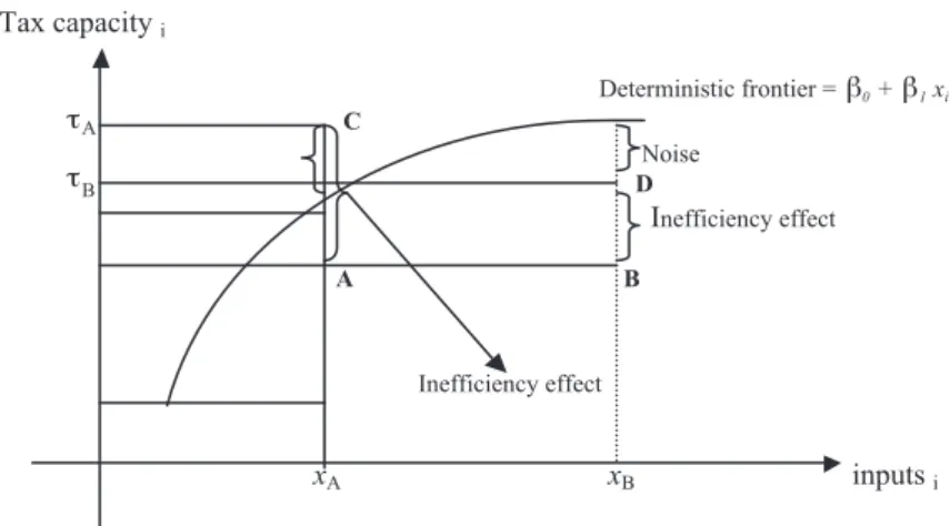
Figure 1 illustrates the main characteristics of the frontier model considering only one independent variable from which tax capacity depends on. If this is the case the model takes the following form:

[2]

whereβ0+β1xiis the deterministic component,viis the noise, anduiis the inefficiency.

The horizontal axis of figure 1 represents the values of inputs (log of GDP and so on) and

the vertical axis the values of the output (log of tax effort). PointsAandBshows the actual

tax revenue of two countries (A and B). Without inefficiencies country A would collectC,and

countryBwould collectD. For country A the noise effect is positive, and then its frontier

revenue is above the deterministic frontier revenue function. On the other hand, for Country B, the noise effect is negative, and then its revenue frontier is under the deterministic frontier

revenue function.1

While frontier revenues are distributed above and below the deterministic frontier revenue function, actual tax revenues are always below this function because the noise effect is positive and larger than the inefficiency effect.

lnτ β βi= +0 1x v ui+ −i i

Figure 1. The Stochastic Production Frontier

The analysis aims to predict and measure inefficiency effects. To do so, we use the tax effort, defined as the ratio between actual tax revenue and the corresponding stochastic frontier tax revenue (tax capacity). This measure of tax effort has a value between zero and one.

[3] The difference between current tax revenue and tax frontier can be interpreted only as the level of unused tax, but not strictly as a measure of inefficiency. The presence of unused tax may be caused by two factors: people’s preferences of low provision of public goods and services, so the low tax revenue is chosen intentionally, and inefficiency of governments in tax collection.

5. Estimation strategy

The estimation is carried out with panel data from an extended list of countries. Methods for estimating stochastic frontiers with panel data are expanding rapidly. These methods are expected to provide “better” estimates of efficiency than those can be obtained from a single cross section, which serves to investigate changes in technical efficiencies over time (as well

as the underlying tax capacity). If observations onuitandvitare independent over time as well

as across countries, then the panel nature of the data set is irrelevant; in fact, cross-section frontier models will apply to the pooled data set, such as the normal-half normal model of Aigner, Lovell and Schmidt (1977) that can be obtained through maximum likelihood estimates. The truncated normal frontier model is due to Stevenson (1980), while the gamma model is due to Greene (1990). The log-likelihood functions for these different models can be found in Kumbhakar and Lovell (2000). But, if one is willing to make further assumptions about the nature of the inefficiency, a number of new possibilities arise. Different structures are commonly classified according to whether they are time-invariant or time-varying.

Time-invariant inefficiency models are somewhat restrictive, and one of the models that allows for time-varying technical inefficiency is the Battese and Coelli (1992) parametrization of time effects (time-varying decay model), where the inefficiency term is modeled as a truncated-normal random variable multiplied by a specific function of time.

[4] where T corresponds to the last time period in each panel, h is the decay parameter to be

estimated, anduiare assumed to have a N(µ,σ) distribution truncated at 0. The idiosyncratic

error term is assumed to have a normal distribution. The only panel-specific effect is the random inefficiency term. Battese and Coelli (1992) propose estimating their models in a random effects framework using the method of maximum likelihood. This often allows us to disentangle the effects of inefficiency and technological change.

The prediction of the technical efficiencies is based on its conditional expectation, and it

is computed by the residual using the formula provided by Jondrowet al(1982), formula

given the observable value of (Vit-Uit).

uit=ui*exp *

[

]

(

)

((

)

(

)

( )

Coelliet al. (2005) suggest that the choice of a more general distribution, such as the truncated-normal distribution, is usually preferable. However, this is ultimately an empirical issue, and we estimate below this specification assuming first the half normal and then the

truncated normal distribution forui.

Heterogeneity

In the development of the frontier model, an important question concerns how to introduce observed heterogeneity into the specification. We assume that there are covariates observed by the econometrician, which are not the direct inputs into tax collection that affect it from the outside, as environmental variables. For example, in the tax capacity case, inflation might impact tax collection and the inefficiency term: countries ability to collect taxes is often influenced by exogenous variables that characterize the environment in which tax collection takes place.

Some authors (e.g., Pitt and Lee, 1981) explored the relationship between environmental variables and predicted technical efficiencies using a two-stage approach. The first stage involves estimating a conventional frontier model with environmental variables omitted. Firm-specific technical efficiencies are then predicted. The second stage involves regressing these predicted technical efficiencies on the environmental variables, usually variables that are observable at the time decisions are made (e.g., degree of government regulation, corruption, and inflation). Failure to include environmental variables in the first stage leads to biased estimators of the parameters of the deterministic part of the production frontier, and also to

biased predictors of technical efficiency.2

A second method for dealing with observable environmental variables is to allow them to directly influence the stochastic component of the production frontier. It is up to the model builder to resolve at the outset whether the exogenous factors are part of the technology heterogeneity or whether they are elements of the inefficiency distribution.

Battese and Coelli (1992, 1995) proposed a series of models that capture heterogeneity and that can be collected in the general form

[5] [6]

andwwiare variables that influence mean inefficiency.

We estimate first Battese and Coelli’s original formulation without heterogeneity with

the base specification g(zit) = exp[–µ(t – T)] and we then estimate a more general formulation,

with g(zit) = exp(µ'zit) and the mean of the truncated normal depending on observable

covariates µi= µ0+ µ1'wi. Notice that z variables influence time-varying inefficiency and wi

variables mean time-invariant inefficiency.

uit =g z U where U N

( )

6. Variables and Data

To determine countries’ tax effort we use a panel dataset that covers 96 countries over 16 years, from 1991 to 2006 (for some countries data was not available for all these years). Once tax effort is determined, we can determine countries’ tax capacity by dividing countries’ tax revenue by countries’ tax effort. We do not include in the analysis countries in which revenue

from hydrocarbons represent more than 30 percent of total tax revenue.3

Dependent Variable

General Tax Revenue as percentage of GDP.The dependent variable chosen is the log of

revenue collected by central and sub national governments as percent of GDP, including social contributions. Source: World Economic Outlook, official websites, and World Bank World Development Indicators (WBWDI). A caveat is worth mentioning: we did not include social security revenue collected and administered by private institutions, but we did include social security revenue collected by the Government. As a consequence, countries such as the USA, with an important level of private social security collection might be closer to its maximum tax capacity than what our analysis shows.

Independent Variables

There are a group of factors that explain countries’ tax effort (and capacity) which are related to the level of income in an economy, how this income is distributed, how ease is to collect taxes, how educated taxpayers are, the degree of openness of an economy, and the level of inflation. Taking into account these factors and the available data we consider that tax effort and capacity) depends on the following variables:

1. Level of development. The first and most common used explanatory variable is the level of development, based on the hypothesis that a high level of development brings more demand for public expenditure (Tanzi 1987) and a higher level of tax capacity to pay for the higher expenditure. Therefore, the expected sign for the coefficient of this variable is positive. The direction of causation between tax capacity and the level of development has been under discussion on several occasions. However, as Tanzi and Zee (2000) suggest it is commonly assumed that income causes taxes, and there is strong international empirical evidence that support this argument. Source data used: GDP per capita, purchasing power parity constant 2005 international $ (GDP PPP, 2005); Source WBWDI.

2. The degree of openness of an economy. As Gupta (2007) expresses the effect of trade

liberalization on revenue mobilization may be ambiguous. When a country begins to open its economy with the reduction of import and exports taxes, and with the increase on exports (usually VAT zero-rate), revenue could be reduced. Furthermore, many countries (such as those of Central America and some of Asia) on opening their economies exempted their exports from income tax.

On the other hand, as Keen and Simone (2004) argue revenue may increase when trade liberalization comes with an improvement in customs procedure. Moreover, on many occasions the reduction of tariff and export taxes come with compensatory measures and revenue does not go down, at least abruptly. In the medium term it is expected that collection increases for more revenue from VAT on imports and more economic activity. To represent the degree of openness of an economy we use trade, imports plus exports as percent of GDP (Trade). Source: WBWDI.

3. The ease of tax collection. The explanatory variable used is the value added of the

agriculture (AVA) sector as percent of GDP (source WBWDI).4 _{Due to political}

reasons some countries exempt agricultural products from VAT as well as agricultural producers from income tax. Moreover, this sector is very difficult to control particularly when it is composed of small producers. Therefore, the expected sign of this variable is negative. Source: WBWDI.

4. Level of Education.More educated people can understand better how and why it is

necessary to pay taxes. With a higher level of education compliance will be higher. Therefore, we expect a positive relationship between this variable and the level of tax effort. Despite the existence of several data, it is sometimes not available for all countries. On other occasions, no variable is useful for comparison. For instance, labor force with secondary education (variable usually used as a proxy to the level of education of countries) (percent of total) was not available for some countries, and secondary education significantly differs among countries. Therefore, as a proxy of the level of education of taxpayers we use the total public expenditure on education percent of GDP (EP). Source: WBWDI.

5. Income distribution. A better income distribution should facilitate collection as well as voluntary taxpayer compliance. The variable used is the GINI coefficient (source WBWDI) which measures the extent to which the distribution of income among individuals deviates from the equal distribution.

6. Inflation. The dependent variable chosen is the percentage change of consumption price index (CPI). As a whole, countries that obtain resources from printing money have negative efficiency for collecting taxes. Therefore, the expected sign for this variable is negative. Source WBWDI.

7. Inefficiencies in collection.There are different inefficiencies that can mean that countries

do not reach their tax frontier. Among them, corruption, weak tax administrations, government ineffectiveness, and low enforcement. We chose only one to represent inefficiencies: the corruption perception index (TICPI), expecting a negative relationship (source: Transparency International).We understand it can represent the mentioned variables as well as it measures the quality of institutions.

As mentioned, the difference between tax capacity and actual revenue includes both inefficiencies and tax policy issues. It is also clear that corruption is an inefficiency and per capita GDP an input. But, the situation is less clear for other variables such as inflation, level of education and income distribution because they can be variables under government control. In our analysis we first include the first sixth variables as inputs, and after we also include corruption as shifting mean inefficiency and inflation influencing time-varying inefficiency.

Table 1

MAIN STATISTICS INDICATTORS OF VARIABLES USED IN THE FRONTIER ANALYSIS

Observations Mean St. Dev. Min Max

General Tax Revenue and Social

Contributions % of GDP 1011 26.0 11.5 6.2 52.6

Trade: Imports plus Exports as percent of GDP 1011 81.9 54.5 14.7 447.3

AVA: Agricultural Sector Value Added 1011 11.6 11.9 0.1 65.1

GDP PPP2005: Per capita GDP 1011 14588.9 13136.3 378.8 72346.0

CPI: Consumer Price Index (% change) 1011 14.9 101.4 –8.2 2075.9

EP: Public Expenditure on Education 1011 4.4 1.6 0.8 9.7

GINI Index 1011 38.4 9.3 24.3 74.3

Log TICPI: Corruption 1011 3.5 1.4 0.5 6.0

7. Empirical Results

We first ran three different specifications for 96 countries pooled from 1991 to 2006 to

obtain baseline specifications.5 _{General government revenue was only available for 53}

countries. For the remaining 43 countries we use central government revenue.

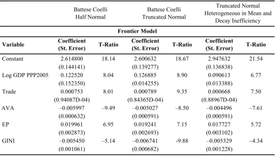
Table 2 shows the maximum likelihood estimation of the parameters of the stochastic frontier tax function for these three specifications. The first one assumes a half normal model, the second a truncated normal, and the third a truncated normal with heterogeneity, such that corruption shifts mean inefficiency and inflation the decay in inefficiency.

Table 2

PARAMETERS OF THE STOCHASTIC FRONTIER TAX FUNCTION. MAXIMUM LIKELIHOOD METHOD

Battese Coelli Battese Coelli _{Heterogeneous in Mean and}Truncated Normal Half Normal Truncated Normal _{Decay Inefficiency}

Frontier Model

Variable Coefficient_{(St. Error)} T-Ratio Coefficient_{(St. Error)} T-Ratio Coefficient_{(St. Error)} T-Ratio

Constant 2.614800 18.14 2.600632 18.67 2.947632 21.54 (0.144141) (0.139277) (0.136838) Log GDP PPP2005 0.122520 8.04 0.126885 8.90 0.090613 6.77 (0.152350) (0.014255) (0.013388) Trade 0.000753 8.01 0.000789 9.35 0.000668 7.50 (0.94087D-04) (0.84365D-04) (0.88967D-04) AVA –0.005997 –9.49 –0.005027 –8.50 –0.004496 –7.61 (0.000632) (0.000591) (0.000591) EP 0.019961 6.95 0.019241 7.15 0.017727 5.72 (0.002873) (0.002693) (0.003102) GINI –0.005450 –5.14 –0.006741 -9.88 –0.005329 –4.34 (0.001061) (0.000682) (0.001228)

Table 2((ccoonnttiinnuueedd))

PARAMETERS OF THE STOCHASTIC FRONTIER TAX FUNCTION. MAXIMUM LIKELIHOOD METHOD

Battese Coelli Battese Coelli _{Heterogeneous in Mean and}Truncated Normal Half Normal Truncated Normal _{Decay Inefficiency}

Inefficiency Constant 0.16485 0.72 0.67464 3.56 (0.22882) (0.18962) LTICPI –0.45068 –2.17 (0.20731) Eta –0.00324 –3.69 (0.00088) CPI 0.00038 2.40 (0.00016) Lambda 7.16535 731.17 6.76492 289.89 6.25998 306.88 (0.00980) (0.02334) (0.02040) Sigma (u) 0.60559 38.34 0.54755 19.91 0.51496 27.43 (0.01579) (0.02750) (0.01877) Log-likelihood 833.44 828.96 836.33

All the coefficients, are statistically significant (different from zero) at 1 percent and have the expected signs. Moreover, in the first and second specification, the coefficients are quite similar as they are the estimated inefficiencies.

In the three models,λi= σui/ σvi, the lambda parameter is quite large, larger than 6 and

statistically significant, implying a large inefficiency component in the model. In fact, dividing the variance of U by the total variance, we get 0.98, which means that 98 per cent of the disturbance term is due to inefficiency.

The third model, where mean inefficiency depends on the level of corruption and the decay on the level of inflation, also maintains the significance, size and sign of the two previous models regarding the inputs to tax effort and capacity. The level of corruption, which is measured from 0.5 (high) to 6 (low), presents a negative sign, meaning that a high level of this variable, that is less corruption, is associated with a lower level of inefficiency. Inflation entered as z in the empirical specification, also increases inefficiency.

7.1. Testing for different specifications

As mentioned above, we run the three previous models using for 53 of the countries revenue from consolidated (general) government and for the other 43 from central government; therefore, we run again the three models allowing for changes in intercept and slopes between countries that reported consolidated revenues (GOV=1) and countries that

reported only revenues from the central government (GOV=0)6_{. A Chow test for structural}

change rejects the hypothesis of no structural change at the 1% confidence level.

Despite the assumption of a more flexible specification, most slopes do not change between the models in table 2 and the models in table 3. The main differences lie on the change in intercept, meaning higher on average tax collection (and frontier) for countries with GOV = 1,

lower slope for AVA, and higher for TRADE for countries with complete tax collection data7_.

The end final result is that tax effort is calculated to be larger than before (and inefficiency smaller) for countries with GOV = 0. Before without controlling for differences in the two group of countries, there was an overestimation on tax inefficiency for the countries with GOV = 0.

Table 3

PARAMETERS OF THE STOCHASTIC FRONTIER TAX FUNCTION WITH STRUCTURAL CHANGE MAXIMUM LIKELIHOOD METHOD

Battese Coelli Battese Coelli _{Heterogeneous in Mean and}Truncated Normal Half Normal Truncated NormaL(a)

Decay Inefficiency(a) Frontier Model

Variable Coefficient_{(St. Error)} T-Ratio Coefficient_{(St. Error)} T-Ratio Coefficient_{(St. Error)} T-Ratio

Constant 2.0935 7.47 1.7223 6.71 2.73090 9.47 (0.2803) (0.2566) (0.28826) Log GDP PPP, 2005 0.1590 5.21 0.1937 6.98 0.09524 3.03 (0.0305) (0.0277) (0.03141) TRADE 0.0012 8.46 0.0015 9.70 0.001245 8.35 (0.0001) (0.00015) (0.000149) AVA –0.0057 –7.16 –0.0054 –6.85 –0.005403 –7.18 (0.0008) (0.0008) (0.000752) EP 0.0159 5.16 0.0145 4.85 0.01433 3.69 (0.0031) (0.0030) (0.00388) GINI –0.0048 –3.45 –0.0040 –2.97 –0.00545 –3.06 (0.0014) (0.0013) (0.001778) GOV 0.5316 1.63 0.8601 2.86 –0.032469 –0.10 (0.3259) (0.3009) (0.341317) LPGOV –0.0398 –1.16 –0.0723 –2.32 0.015085 0.43 (0.0344) (0.0312) (0.035280) AVAGOV 0.0023 1.19 0.0013 0.68 0.004460 2.11 (0.0020) (0.0019) (0.002118) EPGOV 0.0089 1.32 0.0106 1.65 0.010091 1.42 (0.0068) (0.0064) (0.007111) TRAGOV –0.0008 –3.41 –0.0010 –4.77 –0.000864 –3.74 (0.0002) (0.0002) (0.000231) GINGOV –0.0007 –0.35 –0.0012 –0.67 0.000688 0.33 (0.0019) (0.0018) (0.002074)

Table 3((ccoonnttiinnuueedd))

PARAMETERS OF THE STOCHASTIC FRONTIER TAX FUNCTION WITH STRUCTURAL CHANGE MAXIMUM LIKELIHOOD METHOD

Battese Coelli Battese Coelli _{Heterogeneous in Mean and}Truncated Normal Half Normal Truncated NormaL(a)

Decay Inefficiency(a) Inefficiency

Variable Coefficient_{(St. Error)} T-Ratio Coefficient_{(St. Error)} T-Ratio Coefficient_{(St. Error)} T-Ratio

Constant 5.8171 443.5 –7.1780 –0.22 0.49349 2.70 (0.0131) (32.297) (0.18276) LTICPI –0.28618 –1.61 (0.17678) Eta –0.0024 –1.87 –0.0037 –2.77 (0.0013) (0.0013) CPI 0.00051 2.25 (0.00023) Lambda 20.021 195.70 5.03190 182.83 (0.1023) (0.02752) Sigma (u) 0.4949 51.53 1.7036 0.17 0.42363 36.47 (0.0096) (10.188) (0.01162) Log-likelihood 845.11 843.20 848.76

(a) With interactions Dummy GOB. Central GOB revenue = 0, and Total GOB revenue = 1.

Since as mentioned above, it is not clear if the GINI coefficient should be included as input variable or inefficiency influencing variable, we also included the GINI coefficient as a variable that shifts mean inefficiency together with the corruption index. There are no significant changes in the coefficients of all variables (GINI continue being different from zero):

Table 4

PARAMETERS OF THE STOCHASTIC FRONTIER TAX FUNCTION GINI COEFFICIENT INEFFICIENCY INFLUENCING VARIABLE

Truncated Normal Heterogeneous in Mean and Decay Inefficiency

Variable Coefficient (St. Error) T-Radio

LGDPPPP2005 0,08059 0,01427 5,648 Trade 0,00062 0,00009 6,827 AVA –0,54664 0,00059 EP 0,20960 0,32241 0,650 Inefficiency Constant –0,66166 0,26099 –2,535 CPITI –0,21906 0,10776 –2,033 GINI 0,01984 0,00453 4,381 Lambda 4,35217 0,02011 216,425 Sigma 0,36471 0,00483 75,492 CPI 0,00022 0,00017 1,294

Hence, the GINI coefficient could be included both as an input or as influencing inefficiency, the results do not change significantly with respect to ranking of tax capacities, mainly countries with higher levels of inequality have now lower tax capacities.

7.2. Countries Tax Effort

Using the estimates of table 3 we predict tax effort based on the Jondrow, et al. (1982)

formula given the observable value of (Vit- Uit). In table 4, where countries are ranked

according to the value of column VIII, we predicted countries’ tax effort in columns CVII

and CVIII.8 _{In columns IX and X we show countries’ tax capacity. We include the results of}

both the truncated normal model and the truncated normal heterogeneous model. We do not include the results of the half normal model because they are very similar to those of the truncated model.

As expected, countries with a higher level of GDP per capita and public expenditure on education are near their tax capacity, have a higher tax effort. As also expected, agricultural sector and GINI index are also significant variables but with an inverse relationship with tax revenue as percent of GDP.

Tanzi and Davoodi (2000) and Davoodi and Grigorian (2007) find that countries´ institutional quality has a significant relationship with tax revenue, as well as in our study

corruption that summarizes this quality.9_{With regard to inflation, the significance of this}

variable is consistent with findings of Agbeyegbe, Stotsky, and WoldeMariam (2004) and Davoodi and Grigorian (2007).

Our empirical analysis shows that most European Countries with a high level of development are near their tax capacity (have a higher tax effort) defined as the maximum level of tax revenue that a country can achieve taking into account its per capita GDP, GINI coefficient, trade, agricultural sector, education, inflation, and corruption. This is particularly the case of Sweden, France, Italy, Denmark, Finland, Belgium, Hungary, Austria, Netherlands, Slovenia, Norway, and Bulgaria, where, probably, the demand for public expenditure is a crucial determinant of the higher level of tax revenue. Among the 36 countries with the highest level of tax capacity 28 are European (table 5, line 61 to line 96).

Exceptions to this rule are Singapore and Hong Kong, with very high level of per capita GDP and far from their tax capacity (their tax effort are only 23.3% and 28.9%). At least in part, it is a matter of public choice. For instance, Singapore had and has one of the lowest VAT rates, which varied between 3% (1994) and 7% (2008). Something similar we can say about the income tax in China PR, Hong Kong, where the corporate and personal income tax rates are among the lowest in 2008 (16.5% and 17%).

Most of these results are consistent with previous studies. For instance, the significance of per capita GDP is consistent, among others, with Lotz and Mors (1967) and Tanzi (1987).

Ta bl e 5 CO UN TR IE S TA X EF FO RT Ac tu al T ax G DP P PP , Re ve nu e Ta x Ef fo rt Ta x Ca pa cit y Co un tr y Ye ar Re ve nu e (a ) US $ Ce nt ra l = 0 Tr un ca te d Tr un ca te d No rm al % o f G DP 20 05 To ta l = 1 H et er og en eo us Fr om C VI I Fr om C VI II M od el M od el C I C I I C I II (c) C I V C V C V I C V II (c) C V III C I X C X 1. Co ng o, R ep ub lic o f 20 06 6. 3 31 04 .6 0. 0 22 .4 21 .0 28 .1 30 .0 2. Si ng ap or e 20 05 12 .7 43 33 3. 8 0. 0 19 .1 23 .3 66 .8 54 .5 3. Ch in a P .R .: Ho ng K 20 06 16 .6 37 93 7, 7 1. 0 27 .9 28 .9 59 .5 57 .4 4. Su da n 19 99 6. 4 13 08 .9 0. 0 39 .0 31 .9 16 .4 20 .1 5. Ba ng lad es h 20 04 8. 1 10 26 .6 0. 0 43 .7 33 .6 18 .4 24 .1 6. Gu ate m ala 20 05 10 .7 41 01 .9 1. 0 38 .7 35 .8 27 .6 29 .9 7. Ch in a, P. R. : M ain lan d 20 06 14 .9 45 37 .2 1. 0 43 .5 40 .6 34 .3 36 .7 8. Pa ki sta n 20 06 9. 5 22 88 .1 0. 0 49 .7 41 .1 19 .0 23 .0 9. M ad ag as ca r 20 06 10 .7 85 0. 9 0. 0 55 .0 42 .7 19 .5 25 .1 10 . Ve ne zu ela 20 04 16 .2 91 51 .2 0. 0 44 .6 44 .7 36 .3 36 .2 11 . Do m in ica n Re p. 20 05 14 .2 54 30 .0 0. 0 48 .5 45 .3 29 .3 31 .3 12 . Pa na m a 20 01 14 .3 82 19 .3 0. 0 46 .8 47 .1 30 .6 30 .4 13 . Th ail an d 20 06 19 .5 73 78 .4 1. 0 49 .0 47 .6 39 .8 41 .0 14 . In di a 20 05 16 .4 22 29 .9 1. 0 54 .2 48 .7 30 .3 33 .7 15 . M ex ico 20 06 19 .9 11 80 5. 1 1. 0 50 .5 49 .2 39 .4 40 .5 16 . Ca m er oo n 20 06 12 .4 19 79 .7 0. 0 60 .3 50 .3 20 .6 24 .7 17 . M ala ys ia 20 03 18 .8 10 20 8. 7 0. 0 49 .1 50 .3 38 .3 37 .4 18 . El S alv ad or 20 06 15 .3 52 65 .5 0. 0 54 .3 50 .8 28 .1 30 .0 19 . Si er ra L eo ne 20 04 11 .0 56 5. 1 0. 0 69 .8 50 .8 15 .8 21 .7 20 . Bu rk in a F as o 20 06 11 .3 10 50 .6 0. 0 66 .7 51 .9 17 .0 21 .8 21 . Ar m en ia 20 06 17 .1 47 28 .3 1. 0 57 .4 52 .3 29 .7 32 .6 22 . Ko re a 20 06 26 .8 22 30 8. 2 1. 0 53 .6 52 .9 49 .9 50 .6 23 . Pe ru 20 05 15 .3 64 59 .9 0. 0 56 .9 53 .4 26 .9 28 .7 24 . In do ne sia 20 04 12 .8 30 78 .1 0. 0 62 .0 53 .5 20 .6 23 .9 25 . Ph ili pp in es 20 06 14 .3 30 55 .5 0. 0 61 .5 53 .8 23 .2 26 .5 26 . Sr iL an ka 20 05 14 .8 35 45 .9 0. 0 63 .9 55 .3 23 .2 26 .8 27 . Ug an da 20 06 12 .9 86 1. 0 0. 0 66 .5 55 .5 19 .4 23 .2

Ta bl e 5 ((cc oonn ttiinn uuee dd)) CO UN TR IE S TA X EF FO RT Ac tu al T ax G DP P PP , Re ve nu e Ta x Ef fo rt Ta x Ca pa cit y Co un tr y Ye ar Re ve nu e (a ) US $ Ce nt ra l = 0 Tr un ca te d Tr un ca te d No rm al % o f G DP 20 05 To ta l = 1 H et er og en eo us Fr om C VI I Fr om C VI II M od el M od el C I C I I C I II (c) C I V C V C V I C V II (c) C V III C I X C X 28 . Ni ca ra gu a 20 04 21 .5 21 62 .1 0. 0 67 .3 56 .9 31 .9 37 .8 29 . Eg yp t 20 05 14 .1 45 74 .1 1. 0 63 .7 59 .0 25 .1 27 .1 30 . Ho nd ur as 20 06 17 .9 33 27 .2 0. 0 65 .3 59 .0 27 .4 30 .3 31 . Pa ra gu ay 20 06 15 .3 39 09 .3 0. 0 63 .7 59 .3 24 .0 25 .8 32 . M on go lia 20 03 27 .2 22 64 .5 0. 0 71 .0 59 .8 38 .3 45 .5 33 . Ja pa n 20 06 27 .4 30 29 0. 3 1. 0 60 .0 59 .9 45 .7 45 .7 34 . Vi etn am 20 04 21 .5 20 01 .8 1. 0 67 .2 60 .2 32 .0 35 .7 35 . Sw itz er lan d 20 06 30 .1 34 .6 62 .2 1. 0 60 .4 60 .7 49 .8 49 .6 36 . Se ne ga l 20 01 16 .1 14 29 .2 0. 0 70 .1 60 .8 23 .0 26 .5 37 . Jo rd an 20 06 26 .4 45 10 .7 0. 0 67 .8 61 .2 38 .9 43 .1 38 . Ar ge nt in a 20 06 27 .4 11 61 4. 5 1. 0 63 .9 61 .4 42 .9 44 .6 39 . M ali 20 06 15 .5 10 25 .5 0. 0 79 .5 61 .5 19 .5 25 .2 40 . Un ite d St ate s 20 05 27 .3 41 81 3. 2 1. 0 62 .3 62 .2 43 .8 43 .9 41 . Bo liv ia 20 06 26 .6 38 65 .4 1. 0 67 .8 62 .5 39 .2 42 .5 42 . Et hi op ia 20 03 13 .2 52 0. 7 0. 0 88 .9 63 .5 14 .8 20 .8 43 . Gr ee ce 20 06 27 .4 30 40 9. 3 1. 0 65 .2 63 .9 42 .1 42 .9 44 . To go 20 06 14 .6 75 7. 6 0. 0 78 .1 64 .5 18 .7 22 .6 45 . Cô ted ’lv oi re 20 06 16 .6 15 81 .4 0. 0 78 .9 65 .3 21 .1 25 .5 46 . Co sta R ica 20 06 22 .2 96 01 .3 0. 0 67 .9 66 .3 32 .6 33 .4 47 . Tr in id ad an d To ba go 20 05 29 .3 18 14 5. 1 0. 0 65 .8 66 .3 44 .5 44 .1 48 . Ca na da 20 03 28 .5 33 59 8. 7 1. 0 66 .2 66 .6 43 .1 42 .8 49 . Au str ali a 20 05 30 .9 31 .6 56 .1 1. 0 67 .7 66 .8 45 .6 46 .3 50 . Bo tsw an a 20 04 22 .5 11 66 0. 3 0. 0 66 .7 66 .8 33 .7 33 .7 51 . La tv ia 20 06 29 .3 14 91 3. 7 1. 0 69 .3 67 .8 42 .3 43 .2 52 . Sy ria n Ar ab R ep ub lic 19 99 17 .5 37 18 .6 0. 0 76 .6 68 .2 22 .8 25 .7 53 . Ire lan d 20 05 30 .6 37 88 6. 6 1. 0 69 .5 69 .1 44 .0 44 .3 54 . Co lo m bi a 20 03 19 .6 54 98 .1 0. 0 73 .6 69 .2 26 .6 28 .3

Ta bl e 5 ((cc oonn ttiinn uuee dd)) CO UN TR IE S TA X EF FO RT Ac tu al T ax G DP P PP , Re ve nu e Ta x Ef fo rt Ta x Ca pa cit y Co un tr y Ye ar Re ve nu e (a ) US $ Ce nt ra l = 0 Tr un ca te d Tr un ca te d No rm al % o f G DP 20 05 To ta l = 1 H et er og en eo us Fr om C VI I Fr om C VI II M od el M od el C I C I I C I II (c) C I V C V C V I C V II (c) C V III C I X C X 55 . Li th ua ni a 20 06 30 .2 15 25 3. 5 1. 0 71 .4 69 .5 42 .3 43 .4 56 . Ic ela nd 20 05 41 .4 35 46 4. 5 1. 0 71 .8 70 .1 57 .7 59 .1 57 . Ke ny a 20 05 18 .3 13 46 .4 0. 0 87 .3 70 .1 21 .0 26 .1 58 . Gh an a 20 04 22 .4 11 19 .1 0. 0 91 .2 70 .9 24 .6 31 .6 59 . Es to ni a 20 06 30 .8 18 57 8. 3 1. 0 72 .1 71 .1 42 .7 43 .3 60 . Ga m bi a, Th e 20 05 17 .1 99 6. 1 0. 0 89 .6 71 .3 19 .1 24 .0 61 . Ro m an ia 20 05 27 .9 93 67 .6 1. 0 77 .0 72 .9 36 .2 38 .3 62 . Lu xe m bo ur g 20 06 36 .3 72 34 6. 0 1. 0 72 .3 74 .0 50 .2 49 .1 63 . Al ba ni a 20 05 21 .6 54 62 .9 0. 0 81 .3 74 .6 26 .6 29 .0 64 . Sl ov ak R ep ub lic 20 06 29 .6 17 45 2. 3 1. 0 76 .4 75 .5 38 .7 39 .2 65 . Za m bi a 20 06 17 .0 12 33 .4 0. 0 89 .4 77 .0 19 .0 22 .1 66 . So ut h Af ric a 20 06 31 .2 88 06 .7 1. 0 80 .6 77 .1 38 .7 40 .5 67 . Po rtu ga l 20 06 35 .4 20 15 1. 5 1. 0 79 .2 77 .4 44 .7 45 .8 68 . Ne w Ze ala nd 20 02 34 .3 23 51 8. 5 1. 0 80 .6 78 .2 42 .6 43 .9 69 . Sp ain 20 06 37 .2 27 76 7. 9 1. 0 80 .4 78 .8 46 .3 47 .2 70 . Ge rm an y 20 06 35 .7 31 32 3. 2 1. 0 79 .1 78 .9 45 .2 45 .3 71 . Un ite d Ki ng do m 20 06 37 .4 32 04 1. 7 1. 0 80 .3 79 .7 46 .6 47 .0 72 . No rw ay 20 06 43 .6 48 52 5. 9 1. 0 80 .6 80 .7 54 .1 54 .1 73 . Bu lg ar ia 20 06 33 .8 99 76 .8 1. 0 84 .8 81 .2 39 .9 41 .6 74 . Cz ec h Re pu bl ic 20 06 36 .7 21 43 7. 2 1. 0 82 .6 81 .6 44 .5 45 .0 75 . M ol do va 20 06 34 .7 23 21 .6 1. 0 90 .8 82 .7 38 .2 42 .0 76 . Pa pu a N ew G ui ne a 20 02 24 .7 20 49 .1 0. 0 96 .7 84 .2 25 .5 29 .3 77 . Uk ra in e 20 06 36 .6 60 31 .6 1. 0 89 .5 84 .5 40 .9 43 .3 78 . Po lan d 20 05 34 .3 13 57 1. 4 1. 0 87 .5 84 .9 39 .2 40 .4 79 . Sl ov en ia 20 06 39 .4 24 24 8. 8 1. 0 85 .8 85 .1 45 .9 46 .3 80 . Ne th er lan ds 20 06 39 .5 35 41 8. 7 1. 0 85 .9 85 .6 46 .0 46 .1 81 . Ru ss ia 20 06 32 .3 12 79 7. 2 1. 0 89 .2 85 .8 36 .2 37 .6

Ta bl e 5 ((cc oonn ttiinn uuee dd)) CO UN TR IE S TA X EF FO RT Ac tu al T ax G DP P PP , Re ve nu e Ta x Ef fo rt Ta x Ca pa cit y Co un tr y Ye ar Re ve nu e (a ) US $ Ce nt ra l = 0 Tr un ca te d Tr un ca te d No rm al % o f G DP 20 05 To ta l = 1 H et er og en eo us Fr om C VI I Fr om C VI II M od el M od el C I C I I C I II (c) C I V C V C V I C V II (c) C V III C I X C X 82 . Ur ug ua y 20 06 25 .0 98 88 .0 0. 0 89 .0 85 .8 28 .0 29 .1 83 . Tu rk ey 20 06 32 .5 10 94 6. 8 1. 0 91 .0 86 .0 35 .7 37 .8 84 . Au str ia 20 06 41 .9 34 92 9. 9 1. 0 89 .9 89 .3 46 .6 46 .9 85 . Hu ng ar y 20 06 37 .1 17 70 1. 4 1. 0 94 .2 92 .1 39 .4 40 .3 86 . Ja m aic a 20 05 32 .4 59 98 .3 0. 0 95 .8 92 .2 33 .9 35 .2 87 . Na m ib ia 20 03 26 .1 42 26 .4 0. 0 94 .2 92 .5 27 .7 28 .2 88 . Be lg iu m 20 06 45 .4 31 96 8. 7 1. 0 92 .7 92 .6 49 .0 49 .0 89 . De nm ar k 20 06 49 .1 34 59 4. 6 1. 0 95 .2 94 .7 51 .6 51 .8 90 . Fi nl an d 20 06 43 .5 32 00 2. 5 1. 0 96 .0 94 .7 45 .3 45 .9 91 . Br az il 20 06 34 .2 86 73 .1 1. 0 98 .4 95 .1 34 .8 36 .0 92 . Cr oa tia 20 06 40 .2 13 86 7. 1 1. 0 95 .9 95 .3 41 .9 42 .1 93 . Fr an ce 20 06 44 .7 30 95 6. 2 1. 0 96 .6 95 .3 46 .3 46 .9 94 . Ita ly 20 06 42 .7 28 10 8. 9 1. 0 97 .2 95 .8 43 .9 44 .6 95 . Sw ed en 20 06 50 .1 33 14 9. 3 1. 0 98 .4 98 .1 50 .9 51 .0 96 . Be lar us 20 06 45 .7 94 36 .5 1. 0 98 .6 98 .2 46 .4 46 .5 (a ) In clu de s S oc ial C on tri bu tio ns . (b ) W hi le C VI I a nd C IX in clu de 5 d ep en de nt v ar iab les (G DP , A VA , P E, G IN I a nd T ra de ) c ol um n VI II an d X in clu de tw o ad iti on al va ria bl es : i nf lac tio n an d co -rru pt io n. (c ) C III sh ow s t he la st ye ar fo r w hi ch d ata o f a ll va ria bl es o f a co un try w er e a va ila bl e.

Among countries with a low tax effort whose actual tax revenue as percent of GDP is away from their tax capacity we find those with a low level of per capita GDP. Some of these countries have a huge level of exemptions (in some cases established by the Constitutions, such as the case of Guatemala) and others, such as Panama, very low rates. Therefore, in the case of these two countries, public choice explains at least a share of the distance between the actual revenue and the maximum level of revenue that these countries could achieve.

Exceptions to this other rule are Namibia, The Gambia, Kenya, and Ghana with a very low level of per capita GDP but near their tax capacity (high tax effort). Different reasons explain that these countries have this high level of collection and a low per capita GDP. For instance, in the case of The Gambia this is explained by the tax collected on the re-export trade (people who cross the border from neighbor countries to make purchases).

Another crucial issue that our paper estimates is the impact of inefficiencies on collecting taxes. The difference between C VII and C VIII of table 5 shows how tax capacity would increase if corruption and inflation decrease. This is particularly the case of Ghana (whose tax effort would increase 20.3 points –from 70.9 to 91.2– if its level of inflation and corruption were similar to the average of the rest of the countries included in our study), Sierra Leone (19.0), The Gambia (18.3), Mali (18.0), Kenya (17.2), Ethiopia (15.4), Burkina Faso (14.8), Togo (13.6), Côted 'Ivoire (13.5), Bangladesh (11.1), Mongolia (11.1), Nicaragua (10.4), Cameroon (10.0), Moldova (8.1), Pakistan (8.6), and Jordan (6.6).

8. Conclusions

The initial step that a country should follow before implementing new taxes or increasing the rate of the existing ones is to analyze its tax effort, how far its actual revenue is from their tax capacity. If a country is near its tax capacity, then changes in the tax system should be oriented to improve its quality or to mildly increase tax rates. As well, if a country is very near its tax capacity and needs resources to increase its public expenditure it will not be able increase taxes, and this country will need to look for another source of financing, or renounce to such increase of expenditure.

We use a relative method with predictions of tax effort using a comparative analysis of data on these countries. That is to say, the method determines if a country’ tax capacity is high or low in comparison with tax capacity of the other countries, taking into account some characteristics. We use the stochastic frontier tax analysis to determine the tax effort of 96 countries. One of the main differences between the development of production frontier and tax frontier is in the results. In production frontier, the difference between current production and frontier represents the level of inefficiency, something that firms do not accomplish. In tax frontier, the difference between actual revenue and tax capacity includes the existence of technical inefficiencies as well as policy issues (differences in tax legislation, for instance, in the level of rates). We

estimate different specifications of the stochastic frontier using panel data: the Battese-Coelli half normal, truncated normal, and this last incorporating heterogeneity.

Our study corroborates previous analysis inasmuch as the positive and significant relationship between tax revenue as percent of GDP and the level of development (per capita GDP), trade (imports and exports as percent of GDP) and education (public expenditure on education as percent of GDP). The study also demonstrates the negative relationship between tax revenue as percent of GDP and inflation (CPI), income distribution (GINI coefficient), the ease of tax collection (agricultural sector value added as GDP percent), and corruption.

Due to the relationship between tax revenue as percent of GDP (dependent variable) and the independent variables mentioned in the previous paragraph, most European countries with high level of per capita GDP and education, open economies (particularly since the creation of the customs union), low level of inflation and corruption, and strong policies of income distribution have a very high level of tax revenue as percent of GDP, and they are near their tax capacity. This is something that we expected. It is also important to highlight that the high level of their social security contributions is a factor explaining their closeness to tax capacity.

Moreover, the study demostrates:

I As some countries, with a high per capita GDP, have yet capacity to increase their

revenue. This is the case of Hong Kong, Singapore, and Korea countries whose per capita GDP (PPP, 2005) is higher than US$ 20,000 yearly, and whose tax effort varies between 19.1 and 53.6 percent. This does not mean that they have to increase their revenue; this is a public choice issue, these countries can opt for a low level of revenue and public expenditure.

I As several countries with low level of revenue are near their maximum level of collection.

If these countries want to increase their public expenditure (say, to increase their social expenditure) they could not increase tax revenue, and they should look for other resources. This is particularly the case of Ghana, Kenya, and The Gambia whose per capita GDP (PPP, 2005) are lower to US$1,350, and their tax effort higher to 70 percent.

I Some countries that are fare from their tax capacity could increase their revenue

significantly by reducing their inefficiencies (particularly the level of corruption).

Acronyms

AVA Value Added of Agriculture

CPI Consumption Price Index

EP Public Expenditure on Education

GDPPPP2005 Gross Domestic Product per capita, purchasing power parity constant 2005

TICPI The corruption perception index of Transparency International

IMF International Monetary Fund

ML Maximum Likelihood

Notas

1. For a more comprehensive analysis of the stochastic frontier production function see Batesse et al. (2005), Chapter 9.

2. For more details, see Caudill, Ford and Gropper (1995) and Wang and Schmidt (2002).

3. We do not include in the analysis countries in which revenue from hydrocarbons represent more than 30 percent of total tax revenue because a significant portion of revenue from hydrocarbons is classified as nontax revenue (such as royalties or permits to explore). Therefore, tax revenue in these countries is usually low and non tax revenue high, and this affects comparison. For instance, in Kuwait in 2006 while tax revenue was equivalent to 0.9 percent of GDP, nontax revenue (property income) was 47.6 percent of GDP.

4. There were not available data for the 96 countries included in the sample of other variables, such as “time to prepare and pay taxes (hours)”, that can also be proxy of the ease of tax collection.

5. We run the three Battese Coelli specifications shown in Section 5 but we also tried different functional form specifications. Greene (2008) found, consistent with other researchers, that estimates of technical efficiency are quite robust to distributional assumptions, to the choice of fixed or random effects and to methodology, Bayesian vs. classical, but estimates of technical are quite sensitive to the crucial assumption of time invariance. In our case, the estimates were robust to different functional forms and also to the assumption of time invariance. More research remains to be done in studying specifications with true random and fixed effects. 6. The variables LPGOV, AVAGOV, EPGOV, TRAGOV, GINGOV are respectively the original variables Log

GDP PPP2005, AVA, EP, TRADE and GINI multiplied (interacted) by the dummy GOV.

8. The chi squared statistic for the joint test of the hypothesis that the coefficients of the Dummy GOV and the five interaction variables equal zero at the 95% level, is 56.7, 91.8, and 36.7 respectively in each of the models of table III. The Chi Squared with six restrictions is 12.95, clearly lower than any of those statistics, hence rejecting the hypothesis of no structural change.

8. C VII shows tax effort taking into account five dependent variables: GDP, GINI coefficient, trade, agricultural sector, and public expenditure on education. C VIII also shows tax capacity but taking into account two additional independent variables, those that represent inefficiency, inflation and corruption.

9. Salinas and Salinas (2007) using a (i) frontier approach to estimate production frontier (defined as the maximum technically attainable level of production and the associated relative efficiency levels) in a sample of 22 OECD countries during the period 1980–2000 and different corruption indicators showed that this variable negatively affects the efficiency levels at which these economies perform.

Referencias

Agbeyegbe, T.; Stotsky, J. and WoldeMariam, A. (2004), “Trade Liberalization, Exchange Rate Changes, and Tax Revenue in Sub-Saharan Africa”, Working Paper No. 04/178: International Monetary Fund, Washington, DC.

Aigner, D.J.; Lovell, Knox, C.A. and Schmidt, P., “Formulation and Estimation of Stochastic Frontier Production Function Models”, Journal of Econometrics,Vol. 6, 1977: 21-37.

Alfirman, L. (2003), “Estimating Stochastic Frontier Tax Potential: Can Indonesian Local Governments Increase Tax Revenues Under Decentralization?” Department of Economics, University of Colorado at Boulder, Colorado.Working Paper No. 03-19.

Battese, G.E., (1992), “Frontier Production Functions and Technical Efficiencies: A Survey of Empirical Applications in Agricultural Economics”, Agricultural Economics, Vol. 7.

Battese, G., and Coelli, T. (1992), “Frontier Production Functions, Technical Efficiency and Panel Data: With Application to Paddy Farmers in India”, Journal of Productivity Analysis,3: 153-169. Battese, G.E.; Coelli, T.; O’Donnell, C.J.; Timothy J. and Prasada, D.S, (2005), “An Introduction to

Efficiency and Productivity Analysis”. Second Edition. 2005, Springer Verlag.

Caudill, S.; Ford, J. and Gropper, D., (1995), “Frontier Estimation and Firm Specific Inefficiency Measures in the Presence of Heteroscedasticity”, Journal of Business and Economic Statistics, 13: 105-111. Coelli, T., (1992), “A Computer Program for Frontier Production Function Estimation”, Economics

Letters,Vol. 39: 29-32.

Coelli, T.; Rao, D.; O’Donnell, C. and Battese, G., (2005), “An Introduction to Efficiency and Productivity Analysis”, 2nd_{Edition. Springer, ISBN 978-0-387-24266-8.}

Combes, J-L, and Saadi-Sedik, T. (2006), “How Does Trade Openness Influence Budget Deficits in Developing Countries?”, Working Paper 06/03: International Monetary Fund, Washington, DC. Coondo, D.; Majumder, A.; Mukherjee, R. and Neogi, C., (2003), “Tax Performance and Taxable Capacity:

Analysis for Selected States of India”, Journal of Public Finance and Public Choice,Vol. 21: 25-46. Davoodi, H. and Grigorian, D. (2007), “Tax Potential vs. Tax Effort: A Cross-Country Analysis of

Armenia’s Stubbornly Low Tax Collection”, WP/07/106.

Esteller, A. (2003): “La eficiencia en la administración de los tributos cedidos: un análisis explicativo”, Papeles de economía española:320-334.

Greene, W.H., (1990), “A Gamma Distributed Stochastic Frontier Model”, Journal of Econometrics, 46, pp. 141-163.

Greene, W.H. (2008). “The Econometric Approach to Efficiency Analysis”, In The Measurement of Productive Efficiency and Productivity Growth, Fried, H.O.; Knox Lovell, C.A. and Schmidt, S.S. (editors), Oxford University Press,Oxford, Chapter 2: 92-250.

Gupta, A., (2007), “Determinants of Tax Revenue Efforts in Developing Countries”, IMF Working Paper. Jondrow, J.; Materov, I. and Schmidt, P. (1982), “On the Estimation of Technical Inefficiency in the

Stochastic Frontier Production Function Model”, Journal of Econometrics:233-238.

Keen, M.; and Simone, A. (2004), “Tax Policy in Developing Countries: Some Lessons from the 1990s and Some Challenges Ahead,” in Helping Countries Develop: The Role of Fiscal Policy, ed. by Sanjeev Gupta, Benedict Clements, and Gabriela Inchauste. International Monetary Fund, Washington, DC. Kumbhakar, S. and K. Lovell, (2000), “Stochastic Frontier Analysis, Cambridge University Press”.

Cambridge.

Leuthold, J. (1991), “Tax Shares in Developing Economies: A Panel Study,” Journal of Development Economics,35: 173-85.

Lotz, J. and Morrs, E. (1967), “Measuring ‘Tax Effort’ in Developing Countries”, StaffPapers, Vol. 14, No. 3, November 1967: 478-499, International Monetary Fund, Washington, DC.

Pitt, M. and Lee, L. (1981), “The Measurement and Sources of Technical Inefficiency in the Indonesian Weaving Industry”, Journal of Development Economics,9: 43-64.

Salinas-Jimenez, M. and Salinas-Jimenez, J. (2007), Corruption, efficiency and productivity in OECD countries.Instituto de Estudios Fiscales, Universidad de Extremadura. Spain.

Stevenson, R., (1980), “Likelihood Functions for Generalized Stochastic Frontier Estimation”, Journal of Econometrics,13: 58-66.

Stotsky, J. and WoldeMariam, A. (1997), “Tax Effort in Sub-Saharan Africa”, Working Paper 97/107: International Monetary Fund, Washington, DC.

Tanzi, V (1987), “Quantitative Characteristics of the Tax Systems of Developing Countries”, in the theory of Taxation for Developing Countries, edited by David New and Nicholas Stern. New York: Oxford University.

Tanzi, V. and Zee, H.H. (2000), “Tax policy for Emerging Markets: Developing Countries”, International Monetary Fund, Washington, DC, Working Paper/00/35, March 2000.

Tanzi, V. (1987), “Quantitative Characteristics of the Tax Systems of Developing Countries”, in David Newbery and Nicholas Stern (eds), The Theory of Taxation in Developing Countries, Oxford University Press.

Tanzi, V. and H. Davoodi (1997), “Corruption, Public Investment, and Growth”, Working Paper 97/139, International Monetary Fund, Washington, DC.

Varsano, R.; Pessoa, A.; Costa da Silva, N.; Rodrigues Alfonso, J. e Ramundo, J. (1998), “Uma Análise da Carga Tributária do Brasil”, Texto para Discussão nº 583, Rio de Janeiro: IPEA.

Wang, H. and P. Schmidt, (2002), “One Step and Two Step Estimation of the Effects of Exogenous Variables on Technical Efficiency Levels”, Journal of Productivity Analysis,18: 129-144.

Resumen

El presente estudio desarrolla un modelo para determinar el esfuerzo y la capacidad tributaria de 96 países y las principales variables de las cuales, dicho esfuerzo y capacidad, dependen. Los sultados obtenidos permiten determinar qué países se encuentran cerca de su máximo nivel de re-caudación y cuáles no. Nuestro trabajo corrobora estudios previos al encontrar una relación positi-va y significatipositi-va entre el nivel de recaudación medido como porcentaje del PBI y el nivel de desarrollo (PBI per cápita), la apertura económica (importaciones y exportaciones como porcenta-je del PBI) y el nivel de educación de los habitantes de un país (gasto público en educación como porcentaje del PBI). Asimismo, demuestra la relación negativa y significativa entre dicho nivel de recaudación con la inflación (medida a través de la variación en el índice de precios al consumi-dor), la distribución del ingreso (medida a través del coeficiente de GINI), la facilidad de un país para recaudar impuestos (medida a través del valor del producto agropecuario como porcentaje del PBI) y la corrupción.

Palabras clave:esfuerzo tributario, capacidad tributaria, recaudación tributaria, frontera tributaria es-tocástica, ineficiencia.