Munich Personal RePEc Archive
Corruption as Collateral
Ouyang, Min and Zhang, Shengxing
Department of Economics, Tsinghua University School of Economics
and Management, Department of Economics, London School of
Economics
10 February 2020
Online at
https://mpra.ub.uni-muenchen.de/98635/
MPRA Paper No. 98635, posted 15 Feb 2020 14:30 UTC
Corruption as Collateral
∗投
名
状
Min Ouyang† Shengxing Zhang‡ February 10, 2020
Abstract
We propose corruption can substitute for conventional collateral in enforcing financial commit-ments when institutions are poor. A theoretical framework with agency frictions is built, in which corruptive relations with government officials keep firms committed to loan payments. Based on this framework, we hypothesize the anti-corruption investigation destroys the commitment mech-anism so that firms default and, most importantly, firms default strategically as long as they can substitute corruption with other collateral. We investigate regional data and firm-level data from China, and find powerful evidence supporting our hypotheses.
Keywords: Corruption, Relationship lending, Strategic defaults JEL Classification: E44, O16
∗We thank comments and suggestions from Shangjin Wei, Ray Fisman, Yongxiang Wang, John Rogers, Mikhail
Golosov, James Kai-sing Kung, Tao Zha, Zheng Liu, Mark Spiegel, Nobu Kiyotaki, Shouyong Shi, Zhiguo He, Liugang Sheng, Phillips Aghion, Ricardo Reis, James Kai-sing Kung, Alex White, and seminar and conference participants at the 2019 SED, 2019 CEBRA Annual Meetings, the 2019 Tsinghua Workshop of Macroeconomics, HongKong University, the Fanhai International School of Finance of Fudan University, the School of Economics of Fudan University, and the London School of Economics, We especially thank Yiping Wu for assisting estimations in early stages and helped with part of the data collections. Chengzi Yi, Pan Hua, Jingwen Wang provided research assistance. Discussions with Yiping Huang and Xiaochun Liu provided helpful insights. Errors are ours.
†Corresponding author, [email protected], Department of Economics, the School of Economics and
Man-agement, Tsinghua University, Beijing, 100084 China.
1
Introduction
Conventional collateral often fails in unconventional economies. This is captured by a story titled “Ghost Collateral” published by Reuters On May 31st, 2017: bankers in China found some of the col-lateralized physical assets suddenly varnished, some never existed, and some others have been pledged repeatedly to multiple lenders.1
On January 14, 2018, Financial Times reported a similar story: loans in Russia are often issued with fake collateral.2
In these economies, financial contracts are hard to enforce due to various institutional flaws such as loose legal enforcement or hidden credit histories. Yet, the exchange of financial resources is known to be central for economic development (Buera et al.,2011; Moll, 2014). This raises the question how lending occurs where institutions are poor but substantial growth has been achieved.
We propose corruption, a widespread phenomenon in developing/emerging economies, to be an answer. The idea traces back to Leff (1964), Huntington (1968), and Liu (1985) who argue power and bribery can access firms to resources. In this paper, we posit corruptive relations with government officials are essential for firms to get loan resources when institutions are poor. Corruption cases of this kind have been reported as true stories. In 2015, one of the most powerful officials in China named Yongkang Zhou was arrested for corruption; the investigation uncovered he helped an entrepreneur to get a bank loan of 600 million RMB in 2013 as a reward for a bribery of over 14 million RMB.3
In this true story of corruption, banks control the loan resources, the entrepreneur demands loans, and the official connects banks with the entrepreneur for bribes. Like in any corruption cases, bribes incentivize the official. Unlike in many corruption cases where the official offers subsidy or contracts with beneficial pricing to his connected entrepreneurs, here the corrupt official does not control or allocate resources directly, instead he serves the role of financial intermediation.
To sort out the elements of incentivization for banks, entrepreneurs, and officials, formally we build a model of limited commitment. In this model, the entrepreneur has an incentive to distract loan resources to low-quality projects, seize private returns, and avoid debt payment; the bank becomes held up in non-performing loans financing low-quality projects due to the soft-budget constraint; the
1
See “Ghost collateral’ haunts loans across China’s debt-laden banking system” by Reuters.(link).
2
See “How to fix Russia’s broken banking system” by Financial Times (link).
3
According to Pei (2016), the 14 million RMB bribery was paid by an entrepreneur named Liu Han to purchase a tourism project from Zhou’s son, Zhou Bin, at a price of 20 million RMB while the fair market value of the project was under 6 million RMB.
official, however, possesses the power, the information, and the social connections to track credit histories and ban defaulting firms from future loans. Hereby, the entrepreneur and the bank facilitate unsecured lending by forming a corruptive relationship with the official, making the official the de facto intermediary between the two. The continuation value of this relationship for repeated loan issuance corrects the entrepreneur’s distorted incentives, makes unsecured lending safe, and maintains the investment quality. As such, the bribe to the official is nothing but a reward for a much needed service in an environment with poor institutions.
To evaluate the importance of corruption for finance, ideally we would quantify our framework with data to estimate the total amount of corruption-backed loans in reality. Unfortunately, this would be an extremely challenging task, because corruptive activities are known to be secretive, to take various forms, and to be hard to measure properly. Hence, we follow an approach by Fisman (2001), estimating how financial variables respond when corruption is tackled down by the anti-corruption investigation or, in other words, when the corruption channel for finance is blocked. For this purpose, our model provides several testable predictions. It predicts the anti-corruption investigation destroys the corruptive relationship, breaks the commitment, and causes the soft-budget constraint problem to arise for bank-entrepreneur pairs connected with the official under investigation. Consequently, the entrepreneur defaults, leaving the bank with non-performing loans. Moreover, the blocked corruption channel drives the bank to search for yields and the entrepreneurs for alternative financing options. If the entrepreneur can substitute corruption with collateralized borrowing, the default would appear strategic: firm performance stays unaffected, financial status remains intact, but other financing tools are more actively utilized.
We take these predictions to data. Although we believe corruption-backed finance is present ev-erywhere, we choose to examine data from China because in recent years the Chinese government implemented extensive financial reforms to activate more financing tools, providing an ideal institu-tional background for identifying the substitution between corruption and other collateral. Moreover, in 2013 the Chinese president launched an intensive national anti-corruption campaign with an enormous amount of investigations and arrests, generating large data variations for testing our theory. Figure
1 plots the time series of the total number of investigated (“Shuang Gui”) corrupt officials against the ratio of non-performing loans before and after 2013: from 2012 to 2013, the arrests rose by 23%
simultaneously. This is consistent with our theory.
We turn to more detailed panel data to test the true empirical success of our theory. At the regional level, we study the correlation between the amount of non-performing loans and the number of arrested corruption officials. At the firm level, we compile a unique data set on firm defaults and on firm implications by the anti-corruption investigations, combining information publicized by the government and disclosed by news media. With this firm panel, we employ a staggered difference-in-difference approach to estimate a firm’s responses in default probability and in other financial indicators following the arrest of a corrupt official connected with this firm. Our purpose is to identify the true causal relationship stemming from the anti-corruption investigation.
We find robust and powerful evidence supporting our predictions. At the regional level, non-performing loans rise when the anti-corruption campaign intensifies. At the firm level, default prob-ability increases once a firm becomes implicated by the anti-corruption investigation, but the firm’s performance or financial status does not at all deteriorate. We interpret this evidence as a sign of weaker incentives to repay the unsecured debt as implied by our theory, rather than the tightening of their loan-payment capacity as suggested by alternative theories on corruption. Moreover, we find firms turn to share-pledge financing or corporate bonds, and firm value drops accordingly. All these findings point to corruption as an essential financing channel for firms connected with corrupt officials. Our paper is related to several bodies of literature. It joins a recent empirical literature on how the anti-corruption investigation impacts the Chinese economy (Chen and Kung, 2018; Fang et al., 2018, Li et al., 2018). On a broader sense, it belongs to the literature studying the relationship between corruption and growth (Shleifer and Vishny, 1993; Wei, 1999; Olken and Pande, 2012). While this literature often links corruption with slower growth, some scholars have proposed corruption and bribes can work as “grease” to speed up wheels of commerce when regulations are bad (Leff,1964; Huntington,
1968; Liu,1985). Empirically, Mauro (1995) and Svensson (2005) both examine cross-country aggregate data and find evidence suggesting the relationship between corruption and growth is in fact mixed and ambiguous. Our proposed corruption for finance reconciles some of these views.
We also build on the literature on soft-budget constraints faced by financial intermediaries when borrowers’ commitment is limited and the enforcement mechanism is insufficient (Dewatripont and Maskin, 1995, and Maskin and Xu, 2001). We join Boot (2000) to propose relationship lending and specify corruption in particular as a solution for the SBC problem. Our work echos the literature on
contract enforceability and economic institutions (Greif, 1993).
The rest of the paper proceeds as follows. Section 2 builds a model to provide testable predictions. Section 3 discusses the data. Section 4 presents the key evidence. Section 5 explains our evidence is unique to corruption for finance. We conclude in Section 6.
2
Model
We model an environment where monitoring credit is costly and extending credit is risky due to poor institutions. The credit history of an entrepreneur is opaque, either because there lacks a well enforced credit-recording system economy-wide, or because competition among banks and informal creditors fragments credit histories. Therefore, entrepreneurs who defaulted in the past can easily borrow again from new creditors. Pledging conventional physical collateral cannot guarantee the credit safety, as physical assets’ ownerships can be hard to verify. Government officials are powerful: they can track credit histories and influence credit allocations through their extensive connections with entrepreneurs, banks, and other officials.4
This model serves two purposes: to illustrate how corruption supplements poor institutions by enforcing financial commitments and to provide a tractable framework for deriving testable predictions. To achieve these purposes, several elements are required: 1) limited commitment arising from moral hazard that can be overcome by corruption; 2) observable financial instruments that will respond when anti-corruption investigations destroy corruption; 3) testable predictions that can distinguish corruption for financial intermediation from corruption for other economic uses.
2.1 Basic Setups
Time is discrete and lasts forever. The economy is populated by banks, entrepreneurs, and government officials. There are one measure of banks, one measure of entrepreneurs, andNGmeasure of government
officials who participates in lending. All agents have linear utility over consumption. They discount future utility at rate β∈(0,1). The utility from consuming one consumption good is one.
Entrepreneurs use intermediate goods to produce consumption goods. They cannot self finance.
4
Corrupt officials are different from mafia. Gangsters in mafia could punish the defaulting entrepreneur by killing him and his family for example. The punishment that a corrupt official imposes on a defaulting entrepreneur is to terminate an ongoing lending relationship, so that he/she can no longer obtain credit.
In each period, banks are endowed with K units of intermediate goods. Banks can either lend the intermediate goods to entrepreneurs, or invest in a safe storage technology G(K), G being a smooth and concave function with G′′(·)<0< G′(·)< R
H. Individual banks take r0, the return to the
safe-storage technology, as given.5
Denote the amount of intermediate goods banks allocate to safe-storage technology asKS, then:
r0=G′(KS). (1)
An entrepreneurs owns s fraction of her firm’s equity. The measure of entrepreneurs withsshare or less is denoted NE(s), for s∈ [0,1] and NE(1) = 1. We simplify the entry and exit by assuming
an entrepreneur faces an exogenous probability δ of exit at the beginning of every period. An exiting entrepreneur will be replaced by an identical entrepreneur.
Entrepreneurs can form corruptive relationships with government officials for loan issuance. De-veloping such an relationship is a privilege accessible only to a limited number of entrepreneurs. We simplify the entry into corruption by assuming entrepreneurs form such relationships through random matching, under which the probability of meeting an official is evenly distributed among entrepreneurs. Here we abstract away from a potential selection effect of entrepreneurs into corruption (Liu, 1985), because we do not focus on corruption’s allocative impact. In some way, random matching reflects an inefficient allocation of corruptive government connections among entrepreneurs, which is probability true in reality due to corruption’s hidden and secretive nature.
In particular, let the measure of entrepreneurs with share sor less who are connected with officials to be CE
t (s). The rest of entrepreneurs with share s or less, NE(s)−CtE(s), can form relationships
with officials at a probability α∈[0,1]. We assume an official meets at least two entrepreneurs of the same type at the same time when considering a new relationship. Entrepreneurs compete by offering a lump-sum payment upfront to the official. The Bertrand competition implies zero expected value of creating a new relationship for an entrepreneur. After the relationship is established, an entrepreneur will pay an additional flow fee of bribery every period as long as the official stays in power. The amount of the bribe will be determined by Nash bargaining.
5
Even though the banking sector has market power, we assume bankers in each bank compete with each other so that they take as given the bank’s marginal return of lending.
2.2 Soft-budget Constraints
There are of course many ways to model limited commitment arising from moral hazard. In this paper, we follow Dewatripont and Maskin (1995) and Maskin and Xu (2001) to illustrate, without additional enforcement mechanisms, entrepreneurs shirk in maintaining investment quality, which subjects banks to soft-budget constraints.
Each period consists of three sub-periods. At the beginning of sub-period one, an entrepreneur is endowed with a production opportunity that requires one unit of intermediate good. If the opportunity is funded, the entrepreneur makes a choice at sub-period two on the quality of the project to be high or to be low. A high-quality project generates outputRH at the end of sub-period three. RH is fully
pledgeable, and will be seized by the bank in case the entrepreneur defaults. A low-quality project, however, requires one unit of additional funding at sub-period two; it generatesθRLunits of pledgeable
output and(1−θ)RLunits of unpledgeable private return at sub-period three. θ∈(0,1)represents its
pledgeability. The private return cannot be observed by banks, shareholders, or government officials, and therefore will be fully taken by defaulting entrepreneurs.
Assumption 1. RL−r0< RH, r0 < θRL<2r0, RH −r0<(1−θ)RL
RL−r0 < RH ensures the choice of high-quality project to be socially optimal. r0 < θRL makes
sure that banks find it suboptimal to terminate a low-quality project at sub-period two, because the pledgeable part of the output from a low-quality project is higher than its opportunity cost as one additional unit of input.6
θRL <2r0 implies funding low-quality projects generates a loss for banks,
because its pledgeable output is lower than the total amount of funding it requires. Thus, banks keep funding a low-quality project only because the first unit of input is already sunk, and terminating it will generate an even bigger loss. The limited commitment thus generates the classic problem of soft budget constraint (SBC) raised by Dewatripont and Maskin (1995).
RH−r0<(1−θ)RLconcerns the incentive of entrepreneurs withs= 1. Denote the interest rate at
which banks lend to entrepreneurs to ber. Its spread with banks’ opportunity cost r0,r−r0, reflects
the risk premium associated with lending to entrepreneurs. Due to lax institutions, an entrepreneur can default without being punished by continuing to borrow from new creditors, so that she makes her decision based on one-period payoffs only. If she chooses a low-quality project, defaults on the debt,
6
Assumption1takesr0 as given. For the general equilibrium analysis, we assume it holds for all possible value ofr0, r0∈[G′(K), G′(0)].
and runs away, she earns the private return(1−θ)RL. If she chooses a high-quality project and repays
the debt, she retains the residualRH−r. BecauseRH−r0<(1−θ)RLandr0≤r,RH−r <(1−θ)RL
must hold. Therefore, the private return of an entrepreneur with s = 1 from choosing a low-quality project,(1−θ)RL, exceeds her return from a high-quality project,RH −r. The agency friction thus
leads to a socially inefficient quality choice by an entrepreneur with s= 1. For an entrepreneur with
s < 1, the return from enforcing a high-quality project, s(RH −r), is even smaller, but her private
return from a low-quality project remains (1−θ)RL. Therefore, s(RH −r)<(1−θ)RL holds for all
s∈(0,1]. Apparently, a smallersassociates with a more severe moral-hazard problem.
Under Assumption 1, banks expect all entrepreneurs shall choose low-quality projects, subject banks to the SBC, default later, and leave with non-performing loans. In this case, banks will be unwilling to lend due to the SBC, unless there are additional enforcement mechanisms.
2.3 Corruption Enforces Commitment
Due to lax institutions, credit histories are either unobservable or can easily be counterfeited. However, government officials are powerful enough to grant or terminate entrepreneurs’ access to banks. They have wide connections that reach every corner of the society, which gives them a collective memory of entrepreneurs’ credit history as well as extensive capacity to impose punishment. An official, as long as staying in power, can punish a defaulting entrepreneur either by blocking her chances from faking a new credit history or by stopping banks from issuing her new loans. Hereby, government officials become the natural enforcers of financial commitments and the de facto intermediary in the unsecured loan market. They intermediate funding from banks to entrepreneurs in exchange of bribery.
Specifically, for an entrepreneur with sequity share of her firm, let the end-of-period continuation value of her relationship with an official to beW(s), and her end-of-period value in case the relationship terminates to be V(s). Suppose the official charges bribe b(s) when a high-quality project matures. The entrepreneur has the incentive to choose high-quality projects if and only if
(1−θ)RL+V(s)≤s(RH −r)−b(s) +W(s) (2)
The left-hand side of (2) refers to an entrepreneur’s payoff from choosing a low-quality project and defaulting later; the right-hand side is her payoff from choosing a high-quality project and continuing the relationship with the official. When the entrepreneur chooses a low-quality project, the official
terminates the relationship and the entrepreneur is left withV(s)instead ofW(s). Thus,W(s)−V(s)
captures the punishment for a defaulting entrepreneur. If this punishment is greater than her short-run net gain from shirking, (1−θ)RL−s(RH −r), the relationship with the official can correct an
entrepreneur’s short-term incentive and induce her to repay bank loans in full. In this sense, the net continuation value of a corrupt relationship,W(s)−V(s), acts as collateral to back the loan repayment.7
As long as the relationship with the corrupt official generates a social surplus by incentivizing the entrepreneur to choose high-quality projects, the official can share the surplus by charging a bribe,
b(s). The value of b(s) is determined through Nash bargaining. Denote the bargaining power of the entrepreneur to beγ,b(s) satisfies the following:
b(s) = arg max
b {s(RH−r)−b+W(s)−[(1−θ)RL+V(s)]} γ
b1−γ (3)
=(1−γ){[s(RH−r) +W(s)]−[(1−θ)RL+V(s)]}
(3) relatesb(s)to the surplus generated by a corrupt relationship that corrects the short-term incentives of an entrepreneur. It is a fee for the financial intermediation service provided by the official. Together, (2) and (3) suggest the entrepreneur has the incentive to take high-quality projects, to pay a bribe to the corrupt official, and to repay bank loans as long as
(1−θ)RL+V(s)≤s(RH −r) +W(s) (4)
In other words, as long as the surplus of enforcing a high-quality project is positive, the entrepreneur and the corrupt official will find an appropriate value for b(s) so that the incentive constraint for the entrepreneur holds.
2.4 Anti-corruption Investigations
We introduce anti-corruption investigations into the model to allow for disruption of the corruptive lending. Due to anti-corruption investigations, an official faces a probabilityκ∈[0,1]of being arrested and losing power at the beginning of every period. Higher value ofκstands for more intense
investiga-7
Here corruption acts like collateral because entrepreneurs will lose the net gain from corruption if she defaults. However, corruption differs from conventional collateral because, in case of defaults, the conventional collateral value will be seized by the bank but here banks cannot takeW(s)−V(s).
tions.8
We further assume, once the official gets investigated, the connected entrepreneur will forever be prohibited from forming a new corruptive relationship with any other officials unless she exits and re-enters. The continuation value of a corruptive relationship for the entrepreneur, W(s), is
W(s) = ˆβ(1−κ) [s(RH −r)−b(s) +W(s)] + ˆβκ[(1−θ)RL+V(s)] (5)
where βˆ ≡ β(1−δ) denotes the effective discount factor including the firm survival rate. βˆ(1−
κ) [s(RH−r)−b(s) +W(s)]captures the entrepreneur’s payoff from an ongoing relationship, in which
she maintains high-quality projects, bribes the official, and continues as it goes. βκˆ [(1−θ)RL+V(s)]
is an entrepreneur’s payoff if the relationship is terminated by the anti-corruption investigation. Once the official gets investigated and arrested, the entrepreneur deviates to a low-quality project and reaps the private return(1−θ)RL as she anticipates the relationship lending to end. Plugging (3) into (5)
gives
W(s) = ˆβ(1−κ)γ[s(RH−r) +W(s)]
+ ˆβ[1−(1−κ)γ] [(1−θ)RL+V(s)].
Under Condition (4), the value for the entrepreneur increases in her bargaining power γ and de-creases in the intensity of the anticorruption investigationκ. Higher γ raises the share of the surplus allocated to the entrepreneur; higher κ shortens the expected duration of a corruptive relationship.
The interest rater charged by banks includes a premium associated with possible defaults induced by the soft-budget constraint. For simplicity, here we assume banks have little bargaining power over the official, so that the value ofr leaves banks indifferent between lending through the corrupt official and taking the outside optionGthat yields a return ofr0. In the event of the official being investigated
with probabilityκ, the bank funds one more unit to the low-quality project due to the SBC, makes the total amount of lending to be two, and scraps a value of θRL. With probability 1−κ of the official’s
staying in power, no more loan is required and the return to the high-quality project chosen by the entrepreneur is r. Therefore, the expected loan size is(1 +κ). The break-even condition for banks to
8
To keep the model simple, we do not consider additional penalties faced by the corrupt officials after the investigation other than losing briberies.
stay indifferent between the safe outside storage option and lending through the official is
(1 +κ)r0=κθRL+ (1−κ)r. (6)
We can then derive the required return on a corruption-backed loan to be
r= (1 +κ)r0−κθRL
1−κ . (7)
The spread between the return rate to a corruption-backed loan and that to the safe-storage technology,
r−r0, is increasing in anti-corruption intensityκ. Banks charge a higher risk premium whenκis higher.
2.5 Alternative Financing
Now we introduce alternative financing options for the purpose of illustrating the substitution between corruption and more conventional collateral. Alternative financing options can be loans backed by physical assets, loans pledged with equity shares, or corporate-bond issuance. Here we model a a financing tool of particular relevance for our empirical investigations – loans backed by an entrepreneur’s equity shares termed the Share Pledge Finance (SPF). In an economy with poor institutions, physical collateral can be difficult to keep track of, but the ownership and the market value of a publicly listed firm’s equity shares are much easier to verify.
Although the SPF relaxes the borrowing constraint of a share holder, the agency friction between the pledging shareholder and other shareholders is still a concern. Thus borrowing with SPF is costly just as with other forms of collateral. Denote the monitoring cost per unit of loan to be ξ and again assume competitive banks retains no surplus. Then the interest rate at which entrepreneurs borrow through SPF is rp =r0+ξ.9 If SPF is feasible for an entrepreneur with sequity share, the value for
the entrepreneur from SPF is:10
V(s) =sβˆ(RH−rp) + ˆβV(s) =s
ˆ
β(RH−rp)
1−βˆ .
We study the condition under which the SPF incentivizes an entrepreneur to undertake high-quality
9
In China, when the interest rate on bank loans is around 4-5%, the interest rate on SPF could be as high as 8-9%.
10
Here, we simplify the value function without including the future value from being randomly matched with a new corrupt official as, due to the competition for government officials among entrepreneurs, the expected entry value into corruption is zero.
projects. Defaulting on a loan with SPF would reduce an entrepreneur’s shares, driving her to reap private returns from low-quality projects. Thus, her incentive constraint is
(1−θ)RL≤s(RH −rp) +V(s) =
s(RH −rp)
1−βˆ , (8)
In this case, the equity share of an entrepreneur becomes the collateral she would lose in case of defaults. Apparently, (8) holds only for entrepreneurs whose shares are high enough. This requirement on shareholding is consistent with the observed high haircuts on loans with SPF. The punishment from losing equity collateral is more severe if the default leads to a sufficiently high loss of equity shares for the entrepreneur. This imposes a lower bound on the haircut from pledging equity as collateral.
s≥sE = (1−βˆ)(1−θ)RL
RH −r0−ξ
. (9)
Entrepreneurs with s≤sE is unable to borrow against their equity shares. sE is increasing inr0 and
ξ, indicating the measure of entrepreneurs who can borrow against their equity share is decreasing in the opportunity and monitoring cost of borrowing. In summary, the value for a type-sentrepreneur to use SPF is
V(s) = βˆ
1−βˆs(RH −r0−ξ)I(s≥s
E). (10)
Due to lax institutions it costly to monitor collateralized loans, entrepreneurs hence may prefer rela-tionship loans through corrupted officials to collateralized loans. This condition will be derived later. They only switch to collateralized loans when they lose access to corruption backed finance as related officials are investigated. If SPF is the only alternative source of funding, an entrepreneur with share holding less than sE will default in case the anti-corruption investigation instigates her connected
of-ficial, and will forever lose her access to the financial market so that her firm may become a dormant, zombie firm.
2.6 Equilibrium
Before we characterize the equilibrium, a few lemmas should be given and several further assumptions should be made.
enough can borrow, and they borrow through corruption as long as
s≥sCO≡ (1−βˆ)(1−θ)RL
RH−r
. (11)
where r is determined by (7).
Lemma1 posits corruption will become the only tool for finance when the monitoring cost of SPF is too high. G′(K) is the lowest possible value for r
0. When ξ approaches RH −G′(K), the value of
borrowing through SPF would be too low for SPF to be profitable. In that case, only entrepreneurs with equity shares above (11) can overcome the moral-hazard problem and borrow through corruption; those with s below this threshold cannot borrow at all. Higher κ raises this threshold by implying greater risks associated with corruption.
Now we focus on the case when ξ is of appropriate value, so that entrepreneurs have potential access to both corruption and SPF. To focus on the substitution effect between corruption and SPF, we assume all entrepreneurs can borrow with SPF:
Assumption 2. The value of ξ ands is such thats≥sE for all entrepreneurs.
For Assumption 2 to hold, ξ must be of appropriate value for SPF to be profitable. We further assume firms are aware of the moral hazard associated with s so that all entrepreneurs hold enough equity shares to access SPF. In this case, two conditions are required for an entrepreneur to choose corruption over SPF. First, the surplus from corruption must be positive: (1−θ)RL+V(s)≤s(RH−
r) +W(s). Second, the value of utilizing corruption-backed finance must exceed that of using the SPF:
V(s)≤W(s). The precise implications of the two conditions are summarized in Lemma2.
Lemma 2. Under Assumption 2, entrepreneurs with connections to officials utilize corruption for finance if and only if their equity shares meet the following condition:
s≥sC ≡ (1−θ)RL RH −r+ ˆ β 1−βˆξ , (12) where r is determined by (7).
Lemma2suggests the followings. Higherξ lowers the thresholdsC: with higher cost of monitoring
risks associated with corruption, required risk premium for corruption-backed lending increases, so that fewer entrepreneurs can undertake corruption for borrowing.
The equilibrium measure of entrepreneurs connected with corrupt officials is determined by new relationship formation as well as exit induced by the anti-corruption investigation. The law of motion for this measure from periodtto t+ 1is
CE t+1(s) =α NE(s)−NE(sC t )−CtE(s) I(s > sC t )−(κ+δ)CtE(s). (13)
Let CE(s) to denote the steady-state measure of entrepreneurs borrowing through corruption with
equity shares smaller or equal tos. At the steady state,
CE(s) = α 1 +α+κ+δ
NE(s)−NE(sC)
I(s≥sC),
In each period, a fraction κof corruption-backed loans are disrupted, causing entrepreneurs to under-take low-quality projects and forcing banks to lend one more unit of loan resources for each of these projects due to the SBC. Therefore, the expected amount of loans taken by an average project initially financed through corruption is 1−κ+ 2κ = 1 +κ, and the total amount of loans allocated through corruption at periodtis KC
t =CtE(1)(1 +κ). At the steady state, KtC equals
KC = α(1 +κ) 1 +κ+α+δ
1−NE(sC)
. (14)
(14) suggests intensified anti-corruption investigations, captured by higherκ, induces a direct and an indirect effects on the total amount of loans issued through corruption. On the one hand, higher
κ increasesKC: more entrepreneurs plan on defaulting by choosing low-quality projects, which forces
banks to issue additional loans due to the SBC, so that KC rises. This effect is direct. On the other
hand, higher κ causes more exit and discourages entry by raisingsC, so thatKC declines. This effect
is indirect, and takes place with further dynamics in entry and exit. Whenκrises suddenly due to the initiation of the national anti-corruption campaign, it is the direct effect that takes place right away. Since we analyze the steady-state equilibrium only, we make the following assumption to make sure the implications of our comparative-static exercises with higherκ are similar to changes inKC during
Assumption 3. Intermediate inputs occupied by corruption, KC, increases in the anti-corruption intensity κ.
Assumption 3 ensures the direct effect of higher κ dominates: additional loan resources required by more low-quality projects is greater than the decline in the measure of entrepreneurs undertaking corruption for finance. It is meant to capture the on-impact effect of the anti-corruption campaign on non-performing loans.
The equilibrium measure of entrepreneurs who use SPF equals the total amount of loans issued through SPF,KE
t . At the steady state,
KE =KtE = 1− α
1 +α+κ+δ
NE(1)−NE(sC)
,∀t. (15)
To ensure that the equilibrium is well defined, we assume that the total supply of loan resources is large enough:
Assumption 4. K≥1 +κ.
1 + κ is the possibly largest demand for loans: every entrepreneur borrow through corruption and κ fraction requires additional loan resources. Assumption 4 ensures the total loan demand by entrepreneurs is always weakly less than the total supply, so that loan resources allocated to safe-storage technology is nonzero: KS ≥0.
Definition 1. Given the anti-corruption intensity κ, a stationary equilibrium consists of the return rate on safe loans, r0, the return rate on corruption-backed loans, r, the amount of intermediate
inputs allocated to safe storage,KS, to the corruption lending,KC, and to the SPF lending,KE, the
participation threshold for the corruption borrowing, sC, and that for the SPF borrowing, sE, such
that the required return rate on safe loans,r0, clears the loan market:
K =KS+KC +KE.
Moreover,r0 is determined by (1), r by (7), KC by (14),sC by (12),sE by (9), and KE by (15).
The following proposition characterizes the conditions for the existence of a unique stationary equilibrium: it exists when the alternative form of finance is costly, agents are patient enough, and the anti-corruption investigation is not too intensive.
Proposition 1. For ξ > ξ,β > β andκ < κand under Assumptions1, 2, and4, there exists a unique equilibrium where corruption-backed finance is active, entrepreneurs with both connections to officials and access to SFP, choose corruption-backed finance if the entrepreneur’s share holding satisfies (12).
The proof is presented in the appendix. Proposition 1, together with Lemma 1, highlights the implications of institutional frictions on borrowing and lending. In our model, this is captured by the monitoring costξ. When this cost is too high, conventional financing channels are turned off completely (Lemma1). When this cost is sufficiently low, corruption-backed finance may be in-conesequential as in some developed economies. When this cost remains at an intermediate range, both conventional and unconventional financing channels stay active, acting as imperfect substitutes for facilitating economic development.
The next proposition summaries our model’s key predictions to be taken to data for empirical investigations:
Proposition 2. In an equilibrium with all financing channels active, under assumption3, intensifying anti-corruption investigations by raisingκ causes the return on safe investments,r0, to rise and:
1. firm connected with the investigated officials will default, and the amount of non-performing loans will rise.
2. firms connected with the investigated officials will pledge more equity shares for borrowing, their defaults will appear strategic, and their equity value will decline on impact.
The proof is presented in the appendix. Proposition2summarizes two sets of predictions capturing how intensified anti-corruption investigations impact the equilibrium outcome. The first set predicts that, when an corrupt official gets investigated, his corruptive relationships with entrepreneurs terminate so that entrepreneurs default on previous, corruption-backed loans; consequently, non-performing loans rise. The intuition is straightforward: the financial commitments enforced by the corrupt official is broken by his arrest, and entrepreneurs default.
However, alternative theories on corruption can also generate the first set of predictions of Proposi-tion2. In the stories captured by Chen and Kung (2018) and Fang et al. (2018), corrupt officials offer resources like land contracts with favorable pricing or substantial subsidies to their connected firms in exchange of bribes; when these officials get investigated, the connected firms will likely default on
some of the existent loans because losing resources can limit their debt-payment capacity. Therefore, the positive relationship between defaults, non-performing loans and the anti-corruption investiga-tions, although consistent with our theory, does not necessarily prove corruption’s role as financial intermediation.
The second set of predictions of Proposition 2 point to a substitution effect: under Assumption
2, defaulting entrepreneurs substitute corruption with SPF for further borrowing, so that their firms’ operations remain unaffected and their defaults appear strategic. These firms’ equity value drops on impact because SPF is more costly: the entrepreneurs chose corruption over SPF becauseV(s)≤W(s). Moreover, higher κ causes r0 = G′(KS) to rise, because funding held up in non-performing loans
squeezes outKS. Higherr
0 reducesV(s) by raisingrp =r0+ξ, which contributes to a further decline
in firms’ equity value.
The prediction on strategic default is unique to our proposed role of corruption as financial in-termediation. In alternative corruption theories, firms may default with the arrest of the connected officials, but their defaults must accompany deteriorations in performance or financial status. These firms would have no reasons to suddenly default on existent loans if their business is somehow not at all affected by the arrest of the official, unless the official had played a key role in getting those loans. By contrast, firms in our theory default because the arrest of the official breaks the commitment mechanism, regardless of how the anti-corruption investigation impacts firm performance. Whether such defaults appear strategic is conditional on whether these firms can access other financing tools for further resources.
For simplicity, we model SPF as the only alternative financing tool to corruption. But firms can substitute corruption with many other tools for defaults to appear strategic. They can borrow against physical collateral for example. With poor institutions, physical assets are usually hard to verify, and must be another inferior alternative. For similar reasons, corporate bond issuance can be another inferior alternative. When ξ is sufficiently high, as Lemma 1 predicts, all alternative financing tools would shut down completely, leaving corruption the only option for finance.
3
Data
Now we turn to data to investigate the empirical relevance of corruption for finance. For two reasons, we choose to examine data from China, although we believe corruption is utilized for finance in many countries. In 2013, the Chinese president initiated a national anti-corruption campaign that lasted until today. This campaign has generated significant increases in the number of investigations and arrests, resulting in rich data variations to test our predictions. Moreover, the central bank of China has implemented significant financial institutional reforms to activate more financing tools. This provides an ideal institutional background for identifying the substitution effect between corruption and other financial tools as a key component of our theory’s predictions.
We look for two types of data in particular: data on the intensity of anti-corruption investigations or on the identifications of firms implicated by the investigations; and data on financial indicators, especially on firm defaults and on non-performing loans. We compile such data from China at the regional level and at the firm level.
3.1 Regional Data
Our regional panel covers30 Chinese provinces (excluding Tibet) from 2000 to 2015. We focus on two regional indicators.
The first indicator measures regional anti-corruption intensity as the number of officials newly put under investigation for corruption - namely - the “Shuang Gui” officials. This information is published by the 2001-2016 Procuratorial Yearbooks of China.11
We only consider the arrests of “Shuang Gui” officials with bureaucratic ranks at or above the county or division administration level (“Chu Ji”). In principle, this indicator reflects either the amount of regional on-going corruptive activities or the intensity of local anti-corruption investigations. For two reasons, we believe it is changes in the latter rather than in the former that drive variations in this number in China. Firstly, corrupt officials are usually arrested for corruptive activities performed many years ago; Guo (2008) reports the time lag between the year of the occurrence of corruptive activities and the year of their formal investigation to be as long as 5-8 years in China. Secondly, during national anti-corruption campaigns local governors usually make a specific effort to arrest more corrupt officials, because this is a time point when the
11
Procuratorial Yearbooks of China publish statistics of the previous year. For example, the 2001 year book reports activities occurring up until 2000.
central government views increased enforcement figures as an important political achievement and an indication of commitment to the party leader. As shown by Figure1, the number of arrests jumps up sharply at 2013, the year of the initiation of the campaign. It is unlikely that the amount of corruptive activities increased by so much so quickly, especially at a time point right after the Chinese president made an announcement to fight corruption.
The second indicator measures the amount of regional non-performing loans. We compile this data from the 2006-2015 China Banking Regulatory Commission Annual Reports. Non-performing loans are defined as the sum of outstanding “sublime loans”, “dubious loans”, and “damaged loans” held by all financial institutions by the end of the year. A loan is considered “sublime” as long as the borrower has displayed incapacity to make loan payments and the lender expects to recover 50%-70% of the principle; it is considered “dubious” if the lender expects to recover 25% -50% of the principle; it is considered “damaged” if less than 25% of the principle is expected to be recovered. Our data on regional non-performing loans include those borrowed by firms, by all institutions, and by households. Ideally, we would like to have data on non-performing loans borrowed by firms only; unfortunately this data is not available at the regional level. Nonetheless, the 2015 China Banking Regulatory Commission Report documents over 90% of total non-performing loans in China were initially borrowed by firms. Hereby, we use the amount of total non-performing loans to approximate those by firms.
Additionally, we obtain data on regional real GDP growth from the China Statistical Yearbooks. Real GDP growth is calculated as the annual growth in GDP index measured in fixed prices. We us this indicator to control for regional economic activities.
3.2 Firm-level Data
We put together a quarterly panel of 3438 non-financial firms publicly listed in the Shanghai or Shengzhen Stock Exchanges from the first quarter of 2007 to the fourth quarter of 2017. We choose to examine publicly listed firms, because detailed information on their performance and financial status are publicized on a regular base and because they are usually well connected and can access multiple financial tools. Information on firm characteristics, including age, size, and ownership types, and on firm financial status, such as the asset level, cash holdings, and leverage ratio, are from the China Stock Market and Accounting Research Database (CSMAR). This database is considered the Chinese equivalent of the Compustat in the U.S.. The full sample size is 100162. This panel is unbalanced, as
not all firms were present for the entire sample period.
Two data series in this panel are collected on our own. Official records on firm defaults are gathered based on the announcements by the Supreme People’s Court of China. Firms implicated by the anti-corruption investigations, together with the timing of their first implications, are identified according to information publicized by China’s Central Commission Discipline Inspection as well as information reported by news media.
Firm Defaults The Supreme Court of China continually publicizes a list of defaulting firms, called “Shi Xin” firms, together with their specific dates of defaults. The defaulting dates are the days when these firms or some of their branches were ruled by the local court as having failed to fulfill their debt responsibilities. We match this list with our quarterly panel according to firm name, location, and ownership information. In particular, we create a dummy variableSitthat equals one if firmior one of
its branches is announced by the court to have defaulted at least once in quartert, and zero otherwise. This way we are able to identify 437public firms with695records of defaults from 2007 to 2017.
Anti-corruption Implications We identify firms implicated by anti-corruption investigations as follows. Firstly, we collect a sample of corrupt officials based on publicized information on corruption investigation cases. China’s Central Commission of Discipline Inspection continually reports the names and the titles of corrupt officials as well as the specific dates when their investigation cases for corruption were established. Here we restrict our attention to officials at or above the deputy-minister level at the central government or the deputy-governor level at the provincial government, as we believe only higher-level officials can effectively enforce debt commitments.
Secondly, we search for public firms financially linked with the arrested corrupt officials by utilizing Baidu, Yahoo, Bing, and Google search engines. In particular, we apply a search algorithm to collect all the news involving any publicly listed firms as well as the exact names and/or the job titles of any corrupt officials in our sample. Then we manually check each pieces of news, to exclude those reporting activities involving no financial or economic transactions (for example, news saying that the prime minister paid a visit to a factory), and to keep those reporting business transactions (for example, news saying the governor helped a firm to get a loan). The remaining sample yields 128public firms implicated by anti-corruption investigations that were established at various time points, ranging from
the second quarter of 2010 to the fourth quarter of 2017. 12
Based on information obtained as above, we are able to create a dummy variable Cit that equals
one if, in quartert, China’s Central Commission of Discipline Inspection formally establishes an inves-tigation case of an official who has been financially linked with firm i, and zero otherwise.
3.3 Measurements, Trends, and Summary Statistics
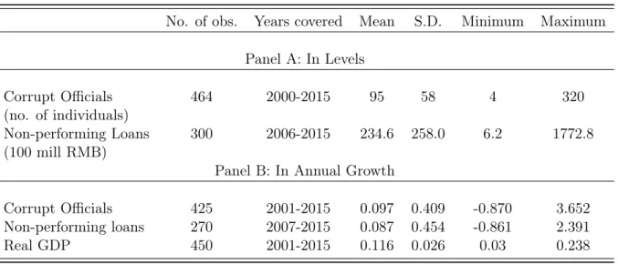
Table1summarizes the regional sample statistics for 30 provinces. Panel A reports statistics in levels. From 2000 to 2015, each province reports an average of95 officials at or above the county or division administration level newly put under formal investigations for corruption every year. The sample on regional performing loans covers the years from 2006 to 2015: the amount of regional non-performing loans averages 23.4billion RMB. Panel B reports statistics in annual growths. From 2000 to 2015, regional “Shuang Gui” officials grew by 9.7% annually, and real GDP grew by 11.6%; from 2006 to 2015, non-performing loans grew by8.7%annually.
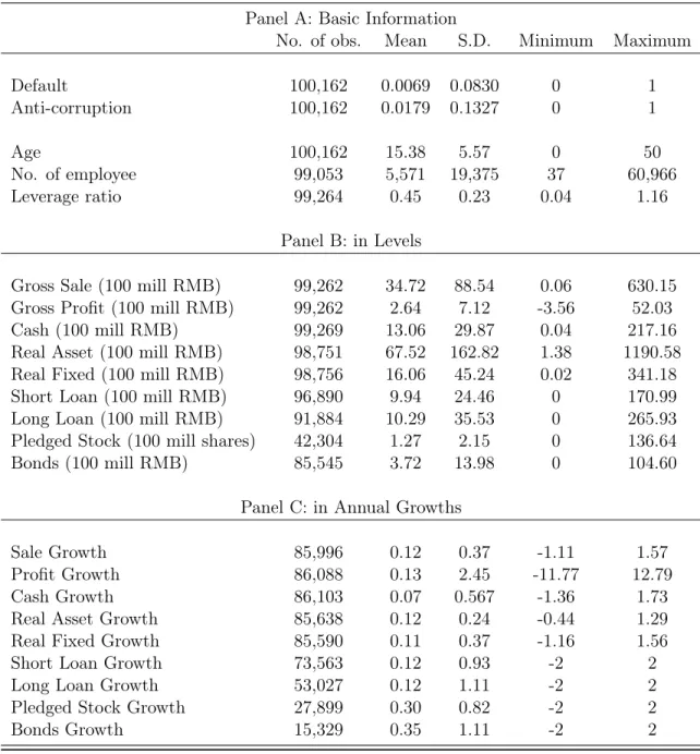
Table2summarizes the firm-level data statistics. Age is defined as the number of years between the year of firms’ registration to the present. The leverage ratio is the ratio of total debts over total assets. Real assets and real fixed assets are calculated by deflating the value of total assets and fixed assets with the provincial fixed-investment price index published by China’s Statistical Year books. Cash is the end-of-the-quarter outstanding level of cash and cash equivalents. Long Loan is the outstanding value of loans borrowed from banks or financial institutions with terms over a year; Short Loan is the value of borrowings with terms within a year.13
We examine two types of financing tools: pledged stock is a quantity measure, as the number of stock shares pledged for borrowing; bonds are the sum of the outstanding principle and interest value of company-issued bonds. All variables are winsorized between 1%and 99%.
According to Panels A and B of Table2, an average publicly listed firm in our sample is fairly large: it employs 5571workers, ages 15.4 years, and displays a leverage ratio of 0.45. It has quarterly sales of 3.47 billion RMB, quarterly profit of 0.26 billion RMB, and cash holdings of 1.31 billion RMB. It holds real assets of 6.8 billion and real fixed assets of 1.6 billion RMB. It carries short-term loans of
12
Li, Wang, and Zhou (2018) examine corruption cases established since 2012 and were able to identify 61 implicated firms. If we also restrict our search to cases after 2012, then we get69implicated firms. The difference in the sample size between our search and theirs may arise from permanent deletion of some old news or more recent news disclosures.
13
The CSMAR database does not specify if short-term loan is borrowed from banks/financial institutions or from other firms/individuals or both.
0.99 billion and long-term loans of 1.03 billion RMB. It has pledged 0.12 billion shares of stocks and issued corporate bonds of 0.37billion RMB.
We apply a measure from Davis and Haltiwanger (1992) to address two data concerns in our sample. Firstly, firm-level variables in China are often non-stationary when measured in levels or log levels, because China experienced extensive institutional reforms as well as frequent policy changes during our sample period. For example, in 2008 China implemented the biggest stimulus packages at the time around the world, causing asset prices to change dramatically in the following years (Ouyang and Peng, 2015). This suggests that we should examine variables measured in growths rather than in levels. Secondly, the conventional growth measures or log-first-difference measures may bias the results by generating value of infinities, because many firm-level variables contain significant number of zero value: for example, the variable “pledged stock” often equals zero, as many firms pledged some equity shares at some point, stopped pledging equity shares for many quarters, and started to pledge equity shares again. Therefore, we follow Davis and Haltiwanger (1992) to measure non-ratio variablesYit as
2 Y it−Yi(t−4) Yit+Yi(t−4) . (16)
(16) measures quarterly annual growth as growth from the same quarter of the last year, which removes any existent seasonalities. Moreover, value of variables measured by (16) stays strictly within
[−2,2]as long asYit is non-negative, and thus avoids the value of infinities.14
Firm Statistics calculated based on (16) are reported in Panel C of Table2: from the first quarter of 2007 to the last quarter of 2017, annual growth rate for an average firm is around 12% for most variables: sales, profits, real assets, real fixed assets, and short-term and long-term loans. For cash holdings, the average annual growth is 7%; for pledged stock and for corporate bonds, the annual growth is around30%.
4
Non-performing Loans and Firm Defaults
With the regional panel and the firm panel, we test our theory’s key predictions captured by Proposition
2. The first null to test is that intensified anti-corruption investigations cause non-performing loans to
14
In Panel C of Table 2, the quarterly annual growth of profit ranges from −0.12 to 12.79 because profit can be negative. Nonetheless, it avoids the value of infinities. When calculating the growth rates of profits based on (16), we take the absolute value of the denominator of (16).
rise, and firms connected with the investigated officials will default accordingly.
4.1 Regional Non-performing Loans
Figure2plots the time series of the average value of regional non-performing loans against the average number of “Shuang Gui” officials across 30 provinces. The former reflects the amount of defaults occurring within an average province. The latter indicates local anti-corruption intensity. The two series should be positively correlated under the null. As shown by Figure 2, both series jump sharply starting from 2013, the year when the national anti-corruption campaign initiated: the average number of regional “Shang Gui” officials rose from96in 2013 to127in 2014 (a32%increase) and to143officials in 2015 (a further 12.5% increase); meanwhile, the average amount of regional non-performing loans rose from18.2 billion RMB in 2013 to26.6 billion RMB in 2014 (a46% increase), and to 40.3billion RMB in 2015 (a further 51.5% increase). The correlation coefficients of the two series is 0.08 before 2008, and0.96 afterward.
However, time-series plots can only be suggestive whether our theory is consistent with the data. Many other factors can generate or mask existent data patterns. For example, in Figure2the amount of non-performing loans declines steadily and sharply between 2005 and 2010, while the number of “Shuang Gui” officials appears relatively stable. This is because since the early 2000s the Chinese government made a successful effort to reduce the large amount of bad loans arising during the 1998 Asia Financial Crisis.15
These strong dynamics can easily cover the positive correlation between the amount of non-performing loans and the number of “Shuang Gui” officials potentially present in the early 2000s. For similar reasons, the seemingly strong correlation between the two series post 2008 can be driven by certain latent common factors.
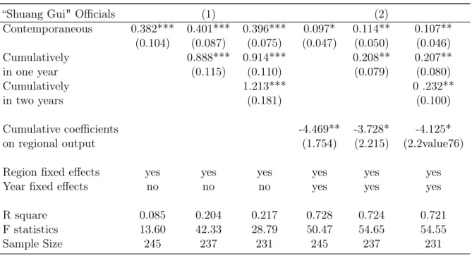
To test the null formally, we run an OLS regression with the regional panel. This allows us to control for some of the aggregate and regional factors. In particular, we test the following specification:
Nit=αi+L(γ)Cit+βXit+ǫit (17)
Nit is the amount of non-performing loans for region i in year t. αi is a regional dummy. L(γ) is a
lag polynomial, Cit is the anti-corruption indicator as the number of “Shuang Gui” officials. Xit is
15
Some remaining bad loans were further eliminated by the debt rollover when the 2008 Stimulus Package was imple-mented (Chen et al.,2019)
a set of controls including year dummies and regional real GDP. ǫit is an error term. All variables
except the dummies are measured in log-first differences (growth rates). The parameter of interest is γ, reflecting the relationship between non-performing loans and the anti-corruption intensity. The regional fixed effect presumably captures the cross-region variations due to long-term economic factors such as culture, industry mix, transportation cost, labor force composition, and etc. Year dummies are to control for the influences of aggregate economic factors such as national fiscal policies, monetary policies, or variations in aggregate economic environment such as the global financial crises. Regional real GDP are to control for other local economic factors. We experiment with various lag lengths as well as with or without controls to check the robustness of our results.
Table 3 presents the OLS regression results of (17). Without controlling for the year dummies or regional GDP, a10%increase in the number of “Shuang Gui” officials is associated with a contempora-neous increase of about 4%in non-performing loans, a cumulative one-year increase of about9%, and a cumulative two-year increase of about12%; all three estimates are significant at the 1%level. After controlling for the year dummies and the regional GDP, the estimated γ’s remain positive, but with reduced point estimates. In particular, a10% increase in the number of “Shuang Gui” officials is asso-ciated with an increase in regional non-performing loans of 1% contemporaneously, 2% cumulatively in one year, and2.3%cumulatively in two years. All estimates onγ stay statistically significant at the
10%level or higher. Also, the estimated coefficients on regional GDP are all negative, consistent with the common belief that non-performing loans rise when local economies turn bad.
The results reported in Table3suggest regional non-performing loans are positively related to local anti-corruption intensities, which supports the null and remains robust after controlling for aggregate and local economic factors. However, there are two limitations in applying the regional data to test the null.
Firstly, variations in Cit, the measured anti-corruption intensity, cannot be fully exogenous. A
positive estimate onγmay not reflect the causality running fromCittoNit, but can be driven by latent
factors causingCit and Nit to co-move. Local economic performance can be one of these factors: bad
economic performance raises non-performing loans and attracts the attention of the central government who pushes local prosecutors to investigate harder, causing more corrupt officials to be arrested. Hereby, regional economic performance creates an upper bias on the estimate for γ; controlling for local GDP corrects for but may not fully eliminate this bias. Also, in 2014 the Chinese government initiated a
plan of “capacity reduction" for heavy-supply industries; officials working in target industries get a lot of investigations. At the same time, firms in these industries experience great difficulty in obtaining new loans, and become more likely to default on existent loans (Chang et al.,2016). In this case,Cit
to Nit rise together for target industries, also generating an upper bias onγ.
Secondly, testing our theory with regional data lacks test power: alternative mechanisms of corrup-tion can generate a positive estimate onγ as well. In our theory, corrupt officials enforce loan payments; the anti-corruption investigation breaks the commitment so that firms default. Hence, intensified in-vestigation arrests more officials, driving more firms to default; consequently, non-performing loans rise. In an alternative theory of corruption, an official exercises power to allocate resources directly under his control – such as tax credit or business permits – to firms in exchange for bribery. If this official gets investigated, his connected firms will lose these resources, which harms firm performance, constrains firms’ debt-payment capacity, and drives firms to default. Intensified investigations arrest more officials, constrain more firms’ debt-payment capacity, and cause non-performing loans to rise with more defaulting firms. Therefore, higher Cit can raise Nit even if corruption never function as
financial intermediation.
4.2 Firm Defaults
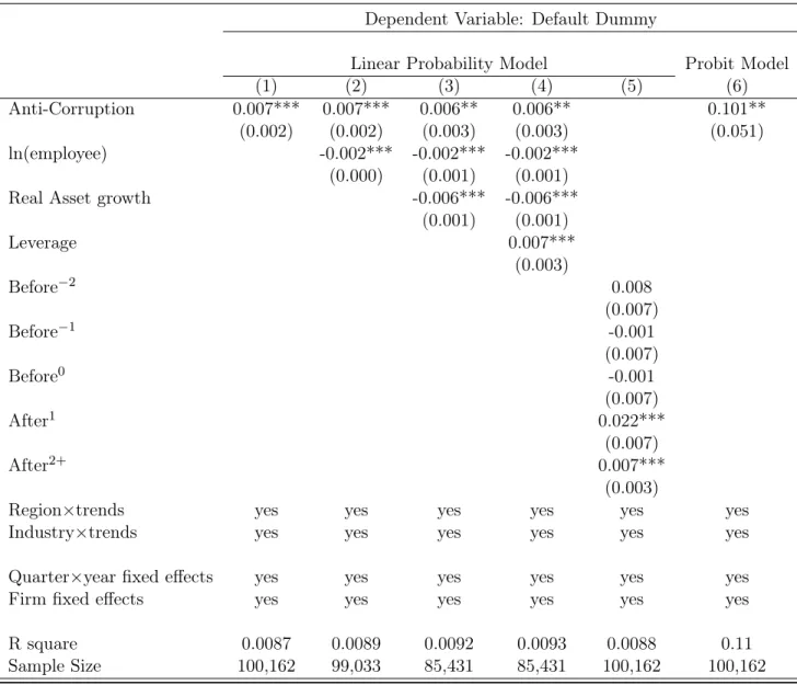
To identify the true causality running from the anti-corruption investigations to defaults, we investigate more detailed firm-level data by performing the following difference-in-difference (DID) estimations:
Sit=αi+αt+γPit+βXit+ǫit (18)
Sit is a default dummy for firm i in quarter t, it equals one if in quarter t firm i or one of its
branches defaults at least once. αi and αt are firm and quarter-year fixed effects. ǫit is an error term.
Pit is a dummy that equals one if an official connected with firm i had been under investigation for
corruption on or before quarter t, and equals zero if the investigation has not yet taken place or will never occur. This is a DID estimation with variations in treatment timing (Bertrand and Mullainathan,
2003). The treated firms are the firms identified to be implicated by the anti-corruption investigation. The staggered occurrence of the corruption cases implies that the corresponding control firms are not restricted to firms never implicated. In fact, Equation (18) takes as a control group all firms that have
notyet been implicated by quarterteven if some will be later. γ is the parameter of interest, capturing the impact of the anti-corruption investigation implication on firm default probability.
In (18),Xit are a set of controls including firm size, the leverage ratio, and real asset growth.
More-over, we include additional province-specific, industry-specific time trends to control for the potential impact of any other policy reforms over the sample period. Firm size is measured as the number of employees in log levels. All other variables except for the leverage ratio and the dummies are measured in quarterly annual growth based on (16). We experiment with and without controlling for firm size, for real asset growth, and for the leverage ratio. All specifications include the standard quarter-by-year and firm fixed effects for the DID estimation.
Our findings are summarized in Table4. Column (1) displays the result of a basic linear probability specification. We find that default probability is about0.7% higher among the implicated firms after their being implicated. Since the average default probability is 0.69% per quarter in our sample, this suggests default probability doubles after being implicated by the anti-corruption investigation. In Columns (2) -(4), we account for several firm characteristics that may be correlated with the fact of being implicated by the anti-corruption investigation. As expected, bigger, larger real-asset-growth, and lower-leverage firms are less likely to default. Accounting for these additional but likely endogenous controls, however, does not change the result that being implicated by the anti-corruption investigation raises default probability by at least0.6%. All estimates are significant statistically at the 5%level or above.
We further investigate issues of reverse causality that may bias our results. As explained earlier, an industry aimed by the government to reduce excessive capacity experience great difficulty in obtaining new loans, and thus more likely to default; meanwhile, government officials taking charge of this industry get plenty of investigations. Likewise, firms located in a province experiencing an economic contraction will default more frequently, which attracts the attention of the investigation agency and causes more local officials to be investigated. Although such possible biases are minimized in our regression by controlling for industry-by-year and province-by-year fixed effects, an alternative way, however, to address reverse causality issues is to examine the dynamic effect of the anti-corruption investigation implication on defaults.
In practice, in column (5) we replace the singleDitdummy with four dummy variables to track the
are dummy variables that equal one for a firm implicated by the anti-corruption investigation two quarters and one quarter prior to the implication, before0 equals one for an implicated firm in that first quarter of being implicated, after1 equals one for an implicate firm that was implicated last quarter,
and after2+ equals one for an implicated firm that was implicated at least two quarters ago. Before−2
and before−1 allow us to assess whether any increased tendency to default can be found prior to the
implication of the anti-corruption investigation. Finding such an “effect” could be a sign of some reverse causality. In fact, we find the estimated coefficient on the before−2 and before−1 dummies both
to be statistically insignificant; the estimated coefficient on before−1 is even negative. This suggests
these implicated firms showed no prior trend of defaulting more than their peers. The estimated effect of the anti-corruption investigation in the quarter of the implication, before0, is still statistically insignificant, probably because it takes several months for the court to reach a ruling on a default. The estimated effect rises to2.2%one quarter after the implication, and remains positive afterward. This is consistent with a causal interpretation of our basic result that a firm is more likely to default after being implicated.
We also check the sensitivity of this result to alternative probability estimation models. Column (6) uses a probit model and finds similar evidence of an increase in default probability following the implication. A logit model delivers similar result that are not reported here.
5
Strategic Defaults
Now we investigate the power of the test of our theory, examining whether our identified defaults caused by anti-corruption implications can differentiate our theory from alternatives. As explained earlier, the anti-corruption investigation can hurt an implicated firm in many ways. In an alternative theory of corruption, an official offers resources directly under his control – such as subsidies or exclusive contracts with favorable pricing – to his connected firms in exchange of bribery. When this official gets arrested, his connected firms experience declines in sales, profits, or cash flows by losing resources, which limits firms’ capacity to pay debts; as a result, default probability rises even if the official never assisted any of these firms in finance. Therefore, the mere finding that the anti-corruption investigation raises defaults cannot differentiate our theory from alternative corruption theories or, put differently, it lacks test power.
Nonetheless, Proposition2gives an unique prediction: firms defaultstrategically following the anti-corruption investigation, as long as the other financing channels are active. That is to say, these firms have the capacity to turn to alternative channels for finance, so that neither their performance nor their financial status are severely impacted after the official loses power. They choose to default on previous, corruption-backed loans, not because they do not have the capacity to pay, but because the arrest of the official breaks the commitment. This prediction is unique to our theory on corruption as a commitment-enforcement mechanism.
In this section, we test the second set of predictions of Proposition2based on our sample of publicly listed firms. As shown by the summary statistics reported in Table 2, our sample firms are big and financially strong. In China, publicly listed firms are usually well connected with access to various financing tools, and are most capable of defaulting strategically. In reality, however, there are many small, private firms that probably have corruption as their only tool for finance. After their being implicated by the anti-corruption investigation, these firms may leave the market once and for all. We purposefully choose not to examine these firms, not only because their data are not as detailed, but also because their lack of capacity for strategic default cannot help differentiate our theory from alternatives.
5.1 Defaults are Strategic
To investigate if our identified defaults are indeed strategic, we estimate how the anti-corruption investigations influence firm performance and financial status, again by exercising a DID estimation:
Yit=αi+αt+γPit+βXit+ǫit (19)
Firm Performance We let Yit in (19) to be gross profit, net profit, gross sales, net sales, and cash
holdings. “Gross" sales or profits calculate the totals of all inflows, while “net" sales or profits consider those from operations only. Pit is the same DID dummy for the anti-corruption implication as in (18).
Xitare a set of control variables: firm size as the number of employees in log levels, real asset growth,
and the leverage ratios. We run DID estimations for each of these performance variables. As usual, all specifications include firm fixed effects, quarter-by-year fixed effects, and additional province-specific,
industry-specific time trends; and all dependent variables are measured as quarterly annual growths.16
The estimation results are reported in Table 5. We find the anti-corruption investigations have negligible influence on most of the performance measures: the four estimated coefficients on the impli-cation dummy for gross sales, net sales, gross profits, and net profits are all statistically insignificant. Cash holdings, however, are estimated to rise by3.07% after a firm becomes implicated. Apparently, none of these results suggest firm performance deteriorates after the arrest of firms’ connected official; as a matter of fact, these firms’ cash holdings appear improved.
We further investigate two sets of accounting variables to explore whether the anti-corruption implications restrain firms’ financial capacity.
Firms’ Ability to Pay Debts The first set of accounting variables measure firms’ ability to pay debts, consisting of five indicators all calculated as fractions of liquid liabilities: Current Rate measures the value of liquid assets; Quick Rate the value of liquid assets net of inventory; Super Quick Rate the value of the sum of cash, short-term securities, and and receivables; Cash Rate 1 the value of net cash flows; and Cash Rate 2 the value of net cash flows from operations only. Higher value of these measures imply more sufficient liquidity to make debt payments. We let Yit to be each of these five
indicators and run DID regressions of (19) one by one.
The results are reported in Panel A of Table6. Maybe surprisingly, we find implicated firms’ ability to pay debts appears stronger after their being implicated: four out of the five estimated coefficients on the implication dummy are positive and statistically significant. These results are consistent with the estimated increase in cash holdings reported in Table 5, implying implicated firms somehow seem to hold more cash or liquid assets relative to their liquid liabilities.
Of course, the fact of being implicated itself cannot give firms more cash or strengthen their debt-payment abilities, since the anti-corruption investigation undoubtedly serves as an adverse shock at least in the short run. We interpret the increase in cash holdings to be an endogenous response, as firms make a specific effort to hedge against risks arising from the anti-corruption implication. Similar results have been reported by Ma et al. (2019), who find Chinese firms hold more cash once exposed to external risks, and by Gao and Xu (2018), who document U.S. firms accumulate more cash during
16
The results in this subsection are based on measurements of the dependent variables calculated following Davis and Haltiwanger (1992). However, alternative measures as log-first difference would generate similar results as long as the performance variable does not contain frequent zero values.