ESSAYS ON
SIMULATION
-BASED
ESTIMATION
Jean-Jacques Forneron
Submitted in partial fulfillment of the
requirements for the degree of
Doctor of Philosophy
in the Graduate School of Arts and Sciences
COLUMBIA UNIVERSITY
2018
c
2018
Jean-Jacques Forneron All rights reserved
ABSTRACT
ESSAYS ONSIMULATION-BASED ESTIMATION
Jean-Jacques Forneron
Complex nonlinear dynamic models with an intractable likelihood or moments are increasingly common in economics. A popular approach to estimating these models is to match informative sample moments with simulated moments from a fully parameter-ized model using SMM or Indirect Inference. This dissertation consists of three chapters exploring different aspects of such simulation-based estimation methods. The following chapters are presented in the order in which they were written during my thesis.
Chapter 1, written with Serena Ng, provides an overview of existing frequentist and Bayesian simulation-based estimators. These estimators are seemingly computationally similar in the sense that they all make use of simulations from the model in order to do the estimation. To better understand the relationship between these estimators, this chapters introduces a Reverse Sampler which expresses the Bayesian posterior moments as a weighted average of frequentist estimates. As such, it highlights a deeper connection between the two class of estimators beyond the simulation aspect. This Reverse Sampler also allows us to compare the higher-order bias properties of these estimators. We find that while all estimators have an automatic bias correction property (as highlighted in Gouri´eroux & Monfort, 1996) the Bayesian estimator introduces two additional biases. The first is due to computing a posterior mean rather than the mode. The second is due to the prior, which penalizes the estimates in a particular direction.
Chapter 2, also written with Serena Ng, proves that the Reverse Sampler described above targets the desired Approximate Bayesian Computation (ABC) posterior distribu-tion. The idea relies on a change of variable argument: the frequentist optimization step implies a non-linear transformation. As a result, the unweighted draws follow a distribu-tion that depends on the likelihood that comes from the simuladistribu-tions, and a Jacobian term that arises from the non-linear transformation. Hence, solving the frequentist estimation problem multiple times, with different numerical seeds, leads to an optimization-based importance sampler where the weights depend on the prior and the volume of the Jaco-bian of the non-linear transformation. In models where optimization is relatively fast, this Reverse Sampler is shown to compare favourably to existing ABC-MCMC or ABC-SMC sampling methods.
Chapter 3, relaxes the parametric assumptions on the distribution of the shocks in simulation-based estimation. It extends the existing SMM literature, where even though the choice of moments is flexible and potentially nonparametric, the model itself is as-sumed to be fully parametric. The large sample theory in this chapter allows for both time-series and short-panels which are the two most common data types found in empir-ical applications. Using a flexible sieve density reduces the sensitivity of estimates and counterfactuals to an ad hoc choice of distribution such as the Gaussian density. Com-pared to existing work on sieve estimation, the Sieve-SMM estimator involves dynami-cally generated data which implies non-standard bias and dependence properties. First, the dynamics imply an accumulation of the bias resulting in a larger nonparametric ap-proximation error than in static models. To ensure that it does not accumulate too much, a set decay conditions on the data generating process are given and the resulting bias is derived. Second, by construction, the dependence properties of the simulated data vary with the parameter values so that standard empirical process results, which rely on a coupling argument, do not apply in this setting. This non-standard dependent empiri-cal process is handled through an inequality built by adapting results from the existing literature. The results hold for bounded empirical processes under a geometric ergod-icity condition. This is illustrated in the paper with Monte-Carlo simulations and two empirical applications.
Contents
List of Figures iii
List of Tables iv
1 The ABC of Simulation-Based Estimation with Auxiliary Statistics 1
1.1 Introduction . . . 2
1.2 Preliminaries . . . 4
1.3 Approximate Bayesian Computation . . . 7
1.4 Quasi-Bayes Estimators . . . 12
1.5 Properties of the Estimators . . . 16
1.6 Two Examples . . . 24
1.7 Conclusion . . . 32
2 A Likelihood-Free Reverse Sample of the Posterior Distribution 33 2.1 Introduction . . . 34
2.2 The Reverse Sampler: CaseK= L . . . 38
2.3 The RS: CaseL≥K: . . . 43
2.4 Acceptance Rate . . . 49
2.5 Conclusion . . . 53
3 A Sieve-SMM Estimator for Dynamic Models 57 3.1 Introduction . . . 58
3.2 The Sieve-SMM Estimator . . . 64
3.3 Asymptotic Properties of the Estimator . . . 71
3.4 Extensions . . . 85
3.5 Monte-Carlo Illustrations . . . 92
3.6 Empirical Applications . . . 100
3.7 Conclusion . . . 108
Appendix to Chapter 1 123
Proof of Proposition 1, RS . . . 123
Proof of Results for LT . . . 126
Results for SLT: . . . 128
Results For The Example in Section 6.1 . . . 131
Further Results for Dynamic Panel Model with Fixed Effects . . . 136
Appendix to Chapter 3 137 Background Material . . . 137
Proofs for the Main Results . . . 146
Additional Asymptotic Results . . . 164
List of Figures
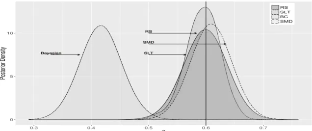
1.1 ABC vs. RS Posterior Density . . . 26
1.2 Frequentist, Bayesian, and Approximate Bayesian Inference forρ . . . 29
1.3 MCMC-ABC vs. RS Posterior Density . . . 31
2.1 Normally Distributed data . . . 54
2.2 The Importance Weights in RS . . . 54
2.3 Exponential Distribution . . . 55
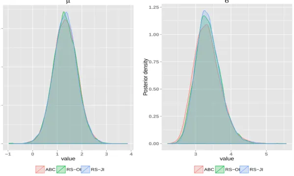
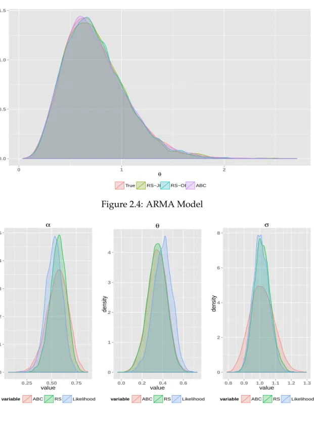
2.4 ARMA Model . . . 55
2.5 Mixture Distribution . . . 56
2.6 Deaton Model: RS and SMD . . . 56
3.1 Static Model: Sieve-SMM vs. Kernel Density Estimates . . . 93
3.2 Autoregressive Dynamics: Sieve-SMM vs. Kernel Density Estimates . . . 95
3.3 Stochastic Volatility: Sieve-SMM vs. Kernel Density Estimates . . . 97
3.4 Dynamic Tobit: Sieve-SMM vs. Kernel Density Estimates . . . 99
3.5 Dynamic Tobit: SMM vs. Sieve-SMM Estimates of the Counterfactual . . . 100
3.6 Industrial Production: Sieve-SMM Density Estimate vs. Normal Density . . . . 102
List of Tables
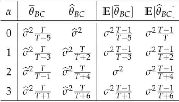
1.1 MeanθBC vs. ModeθbBC . . . 25
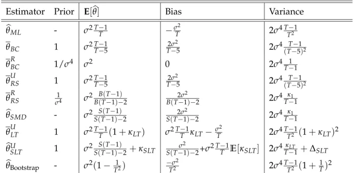
1.2 Properties of the Estimators . . . 27
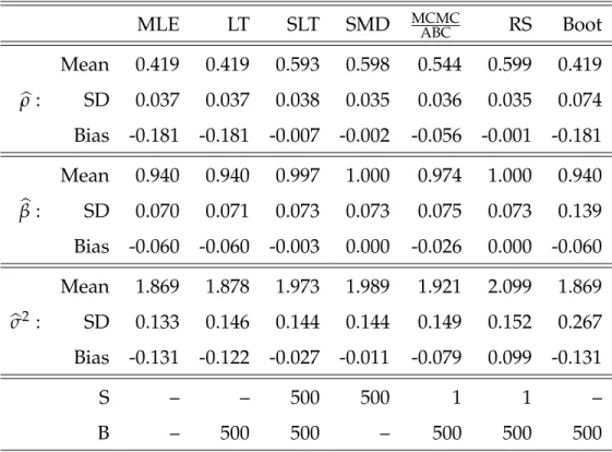
1.3 Dynamic Panelρ=0.6,β=1,σ2=2 . . . 30
2.1 Properties of the Estimators . . . 43
2.2 Acceptance Probability as a function ofδ . . . 50
2.3 Computation Time (in seconds) . . . 52
2.4 Deaton Model: RS, SMD with W=I . . . 53
3.1 Autoregressive Dynamics: Sieve-SMM vs. OLS Estimates . . . 94
3.2 Stochastic Volatility: Sieve-SMM vs. Parametric Bayesian Estimates . . . 96
3.3 Dynamic Tobit: SMM vs. Sieve-SMM Estimates . . . 99
3.4 Industrial Production: Parametric and Sieve-SMM Estimates . . . 102
3.5 Industrial Production: Moments of ∆ct,∆cst andest . . . 103
3.6 Welfare Cost of Business Cycle Fluctuationsλ(%) . . . 104
3.7 Effect of uncertainty on the risk-free rate (% annualized) . . . 105
3.8 Exchange Rate: Bayesian and Sieve-SMM Estimates . . . 107
3.9 Exchange Rate: Moments ofyt,yst andest . . . 109
Acknowledgements
“I would like to conclude with two observations. First, writing a thesis should be fun. Second, writing a thesis is like cooking a pig: nothing goes to waste.” (Umberto Eco,How to Write a Thesis)
During the six years in the making of this thesis, I have come to owe much to my advisor, Serena Ng, for her continuous support and guidance as well as the immense amount of time she has lent me. Long before I discovered the above quote, she taught me to pursue topics of interest to me and to not let any bit of effort go to waste.
I have benefited much from discussions with Jushan Bai, Sokbae Lee, Jos´e Luis Mon-tiel Olea, Christoph Rothe and Bernard Salani´e. Their comments and suggestions have helped shape this thesis into what it is today.
I extremely thankful to my wife, Kim Long-Forneron, for her patience and support throughout these six years as she read through numerous versions of the following chap-ters. Among other things, the writing quality of the following pages would be much degraded without her irreplaceable input.
I would also like to thank my classmates, office neighbours and former students for making these six years memorable. I am particularly thankful to Sakai Ando, Eug´enie Dugoua, Andrew Kosenko, Charles Maurin, Anouch Missirian, Golvine de Rochambeau, Kerem Tuzcuoglu and Jason Wong.
Besides human interactions, I have benefited much from Columbia’s computing facil-ities. In particular, I have abundantly abused the now defunct Yeti and Hotfoot clusters to produce the Monte-Carlo simulations presented in the following chapters.
Chapter 1
The ABC of Simulation-Based
Estimation with Auxiliary Statistics
JEAN-J
ACQUES
FORNERON AND
SERENA
N
G
††Financial support is provided by the National Science Foundation (SES-0962431 and SES-1558623).
We thank Richard Davis for discussions that initiated this research, Neil Shephard, Christopher Drovandi, two anonymous referees, and the editors for many helpful suggestions. Comments from seminar partici-pants at Columbia, Harvard/MIT, UPenn, and Wisconsin are greatly appreciated.
1.1
Introduction
As knowledge accumulates, scientists and social scientists incorporate more and more features into their models to have a better representation of the data. The increased model complexity comes at a cost; the conventional approach of estimating a model by writing down its likelihood function is often not possible. Different disciplines have developed different ways of handling models with an intractable likelihood. An approach popular amongst evolutionary biologists, geneticists, ecologists, psychologists and statisticians is Approximate Bayesian Computation (ABC). This work is largely unknown to economists who mostly estimate complex models using frequentist methods that we generically re-fer to as the method of Simulated Minimum Distance (SMD), and which include such estimators as Simulated Method of Moments, Indirect Inference, or Efficient Methods of Moments.1
The ABC and SMD share the same goal of estimating parameters θ using auxiliary statistics ψb that are informative about the data. An SMD estimator minimizes the L2 distance betweenψband an average of the auxiliary statistics simulated underθ, and this distance can be made as close to zero as machine precision permits. An ABC estimator evaluates the distance betweenψband the auxiliary statistics simulated for eachθdrawn from a proposal distribution. The posterior mean is then a weighted average of the draws that satisfy a distance threshold ofδ >0. There are many ABC algorithms, each differing according to the choice of the distance metric, the weights, and sampling scheme. But the algorithms can only approximate the desired posterior distribution because δ cannot be zero, or even too close to zero, in practice.
While both SMD and ABC use simulations to matchψ(θ)toψb(hence likelihood-free), the relation between them is not well understood beyond the fact that they are asymp-totically equivalent under some high level conditions. To make progress, we focus on the MCMC-ABC algorithm due to Marjoram et al. (2003). The algorithm applies uni-form weights to thoseθsatisfyingkψb−ψ(θ)k ≤δand zero otherwise. Our main insight is that this δ can be made very close to zero if we combine optimization with Bayesian computations. In particular, the desired ABC posterior distribution can be targeted using a ‘Reverse Sampler’ (or RS for short) that applies importance weights to a sequence of SMD solutions. Hence, seen from the perspective of the RS, the ideal MCMC-ABC es-timate with δ = 0 is a weighted average of SMD modes. This offers a useful contrast
1Indirect Inference is due to Gouri´eroux et al. (1993), the Simulated Method of moments is due to Duffie
with the SMD estimate, which is the mode of the average deviations between the model and the data. We then use stochastic expansions to study sources of variations in the two estimators in the case of exact identification. The differences are illustrated using simple analytical examples as well as simulations of the dynamic panel model.
Optimization of models with a non-smooth objective function is challenging, even when the model is not complex. The Quasi-Bayes (LT) approach due to Chernozhukov & Hong (2003) use Bayesian computations to approximate the mode of a likelihood-free objective function. Its validity rests on the Laplace (asymptotic normal) approximation of the posterior distribution with the goal of valid asymptotic frequentist inference. The simulation analog of the LT (which we call SLT) further uses simulations to approximate the intractable relation between the model and the data. We show that both the LT and SLT can also be represented as a weighted average of modes with appropriately defined importance weights.
A central theme of our analysis is that the mean computed from many likelihood-free posterior distributions can be seen as a weighted average of solutions to frequentist objective functions. Optimization permits us to turn the focus from computational to an-alytical aspects of the posterior mean, and to provide a bridge between the seemingly related approaches. Although our optimization-based samplers are not intended to com-pete with the many ABC algorithms that are available, they can be useful in situations when numerical optimization of the auxiliary model is fast. This aspect is studied in our companion paper Forneron & Ng (2016) in which implementation of the RS in the overidentified case is also considered. The RS is independently proposed in Meeds & Welling (2015) with emphasis on efficient and parallel implementations. Our focus on the analytical properties complements their analysis.
The paper proceeds as follows. After laying out the preliminaries in Section 2, Section 3 presents the general idea behind ABC and introduces an optimization view of the ideal MCMC-ABC. Section 4 considers Quasi-Bayes estimators and interprets them from an optimization perspective. Section 5 uses stochastic expansions to study the properties of the estimators. Section 6 uses analytical examples and simulations to illustrate their differences. Throughout, we focus the discussion on features that distinguish the SMD from ABC which are lesser known to economists.2
2The class of SMD estimators considered are well known in the macro and finance literature and with
apologies, many references are omitted. We also do not consider discrete choice models; though the idea is conceptually similar, the implementation requires different analytical tools. Smith (2008) provides a concise overview of these methods. The finite sample properties of the estimators are studied in Michaelides & Ng
1.2
Preliminaries
As a matter of notation, we use L(·) to denote the likelihood, p(·) to denote posterior densities,q(·) for proposal densities, andπ(·)to denote prior densities. A ‘hat’ denotes estimators that correspond to the mode and a ‘bar’ is used for estimators that correspond to the posterior mean. We use (s,S) and (b,B) to denote the (specific, total number of) draws in frequentist and Bayesian type analyses respectively. A superscripts denotes a specific draw and a subscript S denotes the average over S draws. For a function f(θ), we use fθ(θ0)to denote ∂θ∂ f(θ) evaluated atθ0, fθθj(θ0)to denote
∂
∂θjfθ(θ) evaluated atθ0 and fθ,θj,θk(θ0)to denote
∂2
∂θjθkfθ(θ)evaluated atθ0.
Throughout, we assume that the datay = (y1, . . . ,yT)0are strictly stationary and can
be represented by a parametric model with probability measurePθ where θ ∈ Θ ⊂RK. The true value of θ is denoted by θ0. Unless otherwise stated, we write E[·] for
expec-tations taken under Pθ0 instead of EPθ0[·]. If the likelihood L(θ) = L(θ|y) is tractable, maximizing the log-likelihood`(θ) =logL(θ)with respect toθgives
b
θML =argmaxθ`(θ).
Bayesian estimation combines the likelihood with a prior π(θ)to yield the posterior density
p(θ|y) = R L(θ)·π(θ)
ΘL(θ)π(θ)dθ
. (1.1)
For any priorπ(θ), it is known thatbθMLsolves argmax
θ`(θ) =limλ→∞ R
Θθexp(λ`(θ))π(θ)dθ R
Θexp(λ`(θ))π(θ)dθ . That is, the maximum likelihood estimator is a limit of the Bayes estimator usingλ→∞ replications of the data y.3 The parameter λ is the cooling temperature in simulated annealing, a stochastic optimizer due to Kirkpatrick et al. (1983) for handling problems with multiple modes.
In the case of conjugate problems, the posterior distribution has a parametric form which makes it easy to compute the posterior mean and other quantities of interest. For non-conjugate problems, the method of Monte-Carlo Markov Chain (MCMC) allows sampling from a Markov Chain whose ergodic distribution is the target posterior distri-bution p(θ|y), and without the need to compute the normalizing constant. We use the Metropolis-Hastings (MH) algorithm in subsequent discussion. In classical Bayesian
es-(2000). Readers are referred to the original paper concerning the assumptions used.
timation with proposal densityq(·), the acceptance ratio is ρBC(θb,θb+1) =min L(θb+1)π(θb+1)q(θb|θb+1) L(θb)π(θb)q(θb+1|θb) , 1 . When the posterior modeθbBC =argmax
θp(θ|y)is difficult to obtain, the posterior mean θBC = 1 B B
∑
b=1 θb ≈ Z Θθp(θ|y)dθis often the reported estimate, where θb are draws from the Markov Chain upon conver-gence. Under quadratic loss, the posterior mean minimizes the posterior risk Q(a) =
R
Θ|θ−a|2p(θ|y)dθ.
Minimum Distance Estimators
The method of generalized method of moments (GMM) is a likelihood-free frequentist estimator developed in Hansen (1982); Hansen & Singleton (1982). For example, it allows for the estimation ofKparameters in a dynamic model without explicitly solving the full model. It is based on a vector of L ≥ Kmoment conditions gt(θ) whose expected value is zero at θ = θ0, i.e. E[gt(θ0)] = 0. Let g(θ) = T1∑Tt=1gt(θ) be the sample analog of E[gt(θ)]. The estimator is b θGMM = argminθJ(θ), J(θ) = T 2 ·g(θ) 0 Wg(θ) (1.2)
where W is a L×L positive-definite weighting matrix. Most estimators can be put in the GMM framework with suitable choice ofgt. For example, whengt is the score of the
likelihood, the maximum likelihood estimator is obtained.
Letψb≡ψb(y(θ0))beLauxiliary statistics with the property that
√
T(ψb−ψ(θ0))
d
−→N(0,Σ).
It is assumed that the mappingψ(θ) = limT→∞E[ψb(θ)]is continuously differentiable in θ and locally injective at θ0. Gouri´eroux et al. (1993) refer to ψ(θ) as the binding func-tion while Jiang & Turnbull (2004) use the termbridge function. The minimum distance estimator is a GMM estimator which specifies
g(θ) = ψb−ψ(θ),
with efficient weighting matrix W = Σb−1. Classical MD estimation assumes that the binding functionψ(θ)has a closed form expression so that in the exactly identified case, one can solve forθby invertingg(θ).
SMD Estimators
Simulation estimation is useful when the asymptotic binding function ψ(θ0) is not
an-alytically tractable but can be easily evaluated on simulated data. The first use of this approach in economics appears to be due to Smith (1993). The simulated analog of MD, which we will call SMD, minimizes the weighted difference between the auxiliary statis-tics evaluated at the observed and simulated data:
b θSMD = argminθJS(θ) =argminθg 0 S(θ)WgS(θ). where gS(θ) = ψb− 1 S S
∑
s=1 b ψs(ys(θ)),ys(θ)≡ys(εs,θ)are data simulated underθwith errorsεsdrawn from an assumed distri-bution Fε, andψbs(θ) ≡ψbs(ys(εs,θ))are the auxiliary statistics computed usingys(θ). Of course, gS(θ) is also the average overSdeviations between ψband ψbs(ys(θ)). To simplify notation, we will writeys andψbs(θ) when the context is clear. As in MD estimation, the auxiliary statisticsψ(θ)should ‘smoothly embed’ the properties of the data in the termi-nology of Gallant & Tauchen (1996). But SMD estimators replace the asymptotic binding function ψ(θ0) = limT→∞E[ψb(θ0)] by a finite sample analog using Monte-Carlo simu-lations. While the SMD is motivated with the estimation of complex models in mind, Gouri´eroux et al. (1999) show that simulation estimation has an automatic bias reduction effect whenψbis consistent forθ, which is comparable to bootstrap-based bias correction methods. Hence in the econometrics literature, SMD estimators are used even when the likelihood is tractable, as in Gouri´eroux et al. (2010).
The steps for implementing the SMD are as follows:
0 Fors=1, . . . ,S, drawεs = (ε1s, . . . ,εsT)0 fromFε. These are innovations to the struc-tural model that will be held fixed during iterations.
1 Givenθ, repeat fors=1, . . .S:
a Use(εs, θ)and the model to simulate datays = (ys1, . . . ,ysT)0. b Compute the auxiliary statisticsψbs(θ)using simulated datays. 2 Compute: gS(θ) =ψb(y)−1S∑Ss=1ψbs(θ). Minimize JS(θ) = gS(θ)0WgS(θ).
The SMD estimator is the θ that makes JS(θ) smaller than the tolerance specified for the
numerical optimizer. In the exactly identified case, the tolerance can be made as small as machine precision permits. When ψbis a vector of unconditional moments, the SMM
estimator of Duffie & Singleton (1993) is obtained. When ψbare parameters of an auxil-iary model, we have the ‘indirect inference’ estimator of Gouri´eroux et al. (1993). These are Wald-test based SMD estimators in the terminology of Smith (2008). When ψbis the score function associated with the likelihood of the auxiliary model, we have the EMM estimator of Gallant & Tauchen (1996), which can also be thought of as an LM-test based SMD. If ψb is the likelihood of the auxiliary model, JS(θ) can be interpreted as a likeli-hood ratio and we have a LR-test based SMD. Gouri´eroux & Monfort (1996) provide a framework that unifies these three approaches to SMD estimation. Nonparametric esti-mation of the auxiliary statistics was considered in Gallant & Tauchen (1996), Fermanian & Salani´e (2004), Carrasco et al. (2007a), among others. Nickl & P ¨otscher (2011) show that an SMD based on non-parametrically estimated auxiliary statistics can have asymptotic variance equal to the Cramer-Rao bound if the tuning parameters are optimally chosen.4. The Wald, LM, and LR based SMD estimators minimize a weighted L2 distance
be-tween the data and the model as summarized by auxiliary statistics. Creel & Kristensen (2013) consider a class of estimators that minimize the Kullback-Leibler distance between the model and the data.5 Within this class, their MIL estimator maximizes an ‘indirect likelihood’, defined as the likelihood of the auxiliary statistics. Their BIL estimator uses Bayesian computations to approximate the mode of the indirect likelihood. In practice, the indirect likelihood is unknown. Estimating it by kernel smoothing of the simulated statistics, the SBIL estimator combines Bayesian computations with non-parametric es-timation. Gao & Hong (2014) show that using local linear regressions instead of kernel estimation can reduce the variance and the bias. Using non-parametric estimation in ABC has previously been considered in Beaumont et al. (2009). Creel et al. (2016) show that not only can such an ABC implementation bypass MCMC altogether, it can provide asymp-totically valid frequentist inference. Bounds for the number of simulations that achieve the parametric rate of convergence and asymptotic normality are derived.
1.3
Approximate Bayesian Computation
The ABC literature often credits Donald Rubin to be the first to consider the possibility of estimating the posterior distribution when the likelihood is intractable. Diggle & Gratton (1984) propose to approximate the likelihood by simulating the model at each point on
4Similar ideas in statistics include Mitrovic et al. (2016), Park et al. (2016), and Bernton et al. (2017). 5In the sequel, we take the more conventionalL
a parameter grid and appear to be the first implementation of simulation estimation for models with intractable likelihoods. Subsequent developments adapted the idea to con-duct posterior inference, giving the prior an explicit role. The first formal ABC algorithm was implemented by Tavare et al. (1997) and Pritchard et al. (1996) to study population genetics. Their Accept/Reject algorithm is as follows: (i) draw θb from the prior distri-bution π(θ), (ii) simulate data using the model under θb (iii) accept θb if the auxiliary statistics computed using the simulated data are close toψb. As in the SMD literature, the auxiliary statistics can be parameters of a regression or unconditional sample moments. Heggland & Frigessi (2004), Drovandi et al. (2011, 2015) use simulated auxiliary statistics. Since simulating from a non-informative prior distribution is inefficient, subsequent work suggests to replace the rejection sampler by one that takes into account the features of the posterior distribution. The likelihood of the full dataset L(y|θ) is intractable, as is the likelihood of the finite dimensional statistic L(ψb|θ). However, the latter can be con-sistently estimated using simulations. The general idea is to set as a target the intractable posterior density
p∗ABC(θ|ψb)∝ π(θ)L(ψb|θ)
and approximate it using Monte-Carlo methods. Some algorithms are motivated from the perspective of non-parametric density estimation, while others aim to improve properties of the Markov chain.6 The main idea is, however, using data augmentation to consider the joint density pABC(θ,x|ψb) ∝ L(ψb|x,θ)L(x|θ)π(θ), putting more weight on the draws with xclose toψb. Whenx = ψb, L(ψb|ψb,θ)is a constant, pABC(θ,ψb|ψb) ∝ L(ψb|θ)π(θ), and the target posterior is recovered. If ψbare sufficient statistics, one recovers the posterior distribution associated with the intractable likelihoodL(θ|y), not just an approximation.
To better understand the ABC idea and its implementation, we will write yb instead of yb(εb,θb) and ψbb instead of ψbb(yb(εb,θb)) to simplify notation. Let Kδ(ψbb,ψb|θ) ≥ 0 be a kernel function that weighs deviations between ψband ψbb over a window of width δ. Suppose we keep only the draws that satisfy ψbb = ψb and hence δ = 0. Note that
K0(ψbb,ψb|θ) = 1 ifψb = ψbb for any choice of the kernel function. Once the likelihood of interest
L(ψb|θ) =
Z
L(x|θ)K0(x,ψb|θ)dx
is available, moments and quantiles can be computed. In particular, for any measurable
6 Recent surveys on ABC can be found in Marin et al. (2012), Blum et al. (2013) among others. See
function ϕwhose expectation exists, we have: Ehϕ(θ)|ψb=ψbb i = R Θϕ(θb)π(θ)L(ψb|θb)dθb R Θπ(θb)L(ψb|θb)dθb = R Θ R ϕ(θb)π(θb)L(x|θb)K0(x,ψb|θb)dxdθb R Θ R π(θb)L(x|θb)K0(x,ψb|θb)dxdθb . Since ψbb|θb ∼ L(·|θb), the expectation can be approximated by averaging over draws from L(·|bθb). More generally, draws can be taken from an importance density q(·). In particular, b Ehϕ(θ)|ψb=ψb bi = ∑ B b=1ϕ(θb)K0(ψbb,ψb|θb) π(θb) q(θb) ∑B b=1K0(ψbb,ψb|θb) π(θb) q(θb) . The importance weights are then
wb0 ∝K0(ψbb,ψb|θb) π(θb)
q(θb). By a law of large numbers,Eb
ϕ(θ)|ψb →E ϕ(θ)|ψb asB→∞.
There is, however, a caveat. When ψbhas continuous support, ψbb = ψbis an event of measure zero. ReplacingK0withKδwhereδis close to zero yields the approximation:
Ehϕ(θ)|ψb=ψb bi ≈ R Θ R ϕ(θb)π(θb)L(x|θb)Kδ(x,ψb|θb)dxdθb R Θ R π(θb)L(x|θb)Kδ(x,ψb|θb)dxdθb .
SinceKδ(·)is a kernel function, consistency of the non-parametric estimator for the con-ditional expectation of ϕ(θ) follows from, for example, Pagan & Ullah (1999). This is the approach considered in Beaumont et al. (2009), Creel & Kristensen (2013) and Gao & Hong (2014). The case of a rectangular kernelKδ(ψb,ψbb) = Ik
b
ψ−ψbbk≤δ corresponds to the
ABC algorithm proposed in Marjoram et al. (2003). This is the first ABC algorithm that exploits MCMC sampling. Hence we refer to it as MCMC-ABC. Our analysis to follow is based on this algorithm. Accordingly, we now explore it in more detail.
Algorithm MCMC-ABC Letq(·) be the proposal distribution. Forb = 1, . . . ,Bwith θ0 given,
1 Generateθb+1 ∼q(θb+1|θb).
2 Drawεb+1from Fε and simulate datayb
+1. Compute
b ψb+1.
3 Accept θb+1 with probabilityρABC(θb,θb+1) and set it equal toθb with probability
1−ρABC(θb,θb+1)where ρABC(θb,θb+1) =min Ikψb−ψbb+1k≤δ π(θb+1)q(θb|θb+1) π(θb)q(θb+1|θb) , 1 . (1.3)
As with all ABC algorithms, the success of the MCMC-ABC lies in augmenting the pos-terior with simulated data ψbb, i.e. p∗ABC(θb,ψbb|ψb) ∝ L(ψb|θb,ψbb)L(ψbb|θb)π(θb). The joint posterior distribution that the MCMC-ABC would like to target is
p0ABCθb,ψb b| b ψ ∝π(θb)L(ψb b| θb)Ik b ψb−ψbk=0
since integrating outεb would yield p∗ABC(θ|ψb). But it would not be possible to generate draws such thatkψbb−ψbkequals zero exactly. Hence as a compromise, the MCMC-ABC algorithm allowsδ >0 and targets
pδ ABC θb,ψb b| b ψ ∝π(θb)L(ψb b| θb)Ik b ψb−ψbk≤δ. The adequacy ofpδ
ABC as an approximation ofp0ABCis a function of the tuning parameter
δ.
To understand why this algorithm works, we follow the argument in Sisson & Fan (2011). If the initial draw θ1 satisfies kψb−ψb1k ≤ δ, then all subsequent b > 1 draws are such thatIk
b
ψb−ψbk≤δ = 1 by construction. Furthermore, since we drawθ
b+1and then
independently simulate dataψbb+1, the proposal distribution becomes q(θb+1,ψbb+1|θb) = q(θb+1|θb)L(ψbb+1|θb+1). The two observations together imply that
Ikψb−ψbb+1k≤δ π(θb+1)q(θb|θb+1) π(θb)q(θb+1|θb) = Ikψb−ψbb+1k≤δ Ikψb−ψbbk≤δ π(θb+1)q(θb|θb+1) π(θb)q(θb+1|θb) L(ψbb +1| θb+1) L(ψbb|θb) L(ψbb|θb) L(ψbb+1|θb+1) = Ikψb−ψbb+1k≤δ Ikψb−ψbbk≤δ π(θb+1)L(ψbb+1|θb+1) π(θb)L(ψbb|θb) q(θb|θb+1)L(ψbb|θb) q(θb+1|θb)L(ψbb+1|θb+1) = p δ ABC θb +1, b ψb+1|ψb pδ ABC θb,ψbb|ψb q(θb,ψbb|θb +1) q(θb+1,ψbb+1|θb) .
The last equality shows that the acceptance ratio is in fact the ratio of two ABC posteriors times the ratio of the proposal distribution. Hence the MCMC-ABC effectively targets the joint posterior distribution pδ
ABC.
The Reverse Sampler
Thus far, we have seen that the SMD estimator is theθthat makeskψb−1S∑sS=1ψbs(θ)kno larger than the tolerance of the numerical optimizer. We have also seen that the feasible MCMC-ABC accepts draws θb satisfying kψb−ψbb(θb)k ≤ δ with δ > 0. To view the MCMC-ABC from a different perspective, suppose that settingδ =0 was possible. Then each accepted drawθb would satisfy:
b
For fixedεb and assuming that the mappingψbb : θ →ψbb(θ)is continuously differentiable and one-to-one, the above statement is equivalent to:
θb =argminθ b ψb(θ)−ψb 0 b ψb(θ)−ψb .
Hence each accepted θb is the solution to a SMD problem with S = 1. Next, suppose that instead of drawing θb from a proposal distribution, we draw εb and solve for θb as above. Since the mappingψbb is invertible by assumption, a change of variable yields the relation between the distribution ofψbbandθb. In particular, the joint density, sayh(θb,εb), is related to the joint densityL(ψbb(θb),εb)via the determinant of the Jacobian |ψbbθ(θb)|as follows:
h(θb,εb|ψb) = |ψbbθ(θb)|L(ψbb(θb),εb|ψb).
Multiplying the quantity on the right-hand-side by wb(θb) = π(θb)|ψbb θ(θ
b)|−1 yields
π(θb)L(ψb,εb|θb)sinceψbb(θb) = ψband the mapping fromθb toψb(θb) is one-to-one. This suggests that if we solve the SMD problem B times each with S = 1, re-weighting each of the B solutions by wb(θb) would give the target the joint posterior p∗ABC(θ|ψb) after integrating outεb.
Algorithm RS
1 Forb =1, . . . ,Band a givenθ,
i Drawεb fromFεand simulate dataybusingθ. Computeψbb(θ)fromyb. ii Letθb =argminθJ1b(θ), J1b(θ) = (ψb−ψbb(θ))0W(ψb−ψbb(θ)).
iii Compute the Jacobianψbθb(θb)and its determinant|ψbbθ(θb)|. Letwb(θb) = π(θb)|ψbb
θ(θ
b)|−1.
2 Compute the posterior meanθRS =∑Bb=1wb(θb)θbwherewb(θb) =
wb( θb) ∑B
c=1wc(θc)
. The RS has the optimization aspect of SMD as well as the sampling aspect of the MCMC-ABC. We call the RS the reverse sampler for two reasons. First, typical Bayesian esti-mation starts with an evaluation of the prior probabilities. The RS terminates with the evaluation of the prior. Furthermore, we use the SMD estimates to reverse engineer the posterior distribution.
Consistency of each RS solution (i.e. θb) is built on the fact that the SMD is consistent even with S = 1. The RS estimate is thus an average of a sequence of SMD modes. In contrast, the SMD is the mode of an objective function defined from a weighted average of the simulated auxiliary statistics. Optimization effectively allows δ to be as close to
zero as machine precision permits. This puts the joint posterior distribution as close to the infeasible target as possible, but has the consequence of shifting the distribution from
(yb,ψbb) to(yb,θb). Hence a change of variable is required. The importance weight de-pends on the Jacobian matrix, making the RS an optimization based importance sampler. Lemma 1. Suppose thatψ: θ →ψbb(θ)is one-to-one andψb
θ(θ)has full column rank. The poste-rior distribution produced by the reverse sampler converges to the infeasible posteposte-rior distribution p∗ABC(θ|ψb)as B→∞.
The proof is given in Forneron & Ng (2016). By convergence, we mean that for any measurable functionϕ(θ)such that the expectation exists, a law of large numbers implies that ∑Bb=1wb(θb)ϕ(θb)
a.s.
−→Ep∗(θ|
b
ψ)(ϕ(θ)). In general, wb(θb) 6= 1B. The RS draws and
moments can be interpreted as if they were taken from pABC∗ , the posterior distribution had the likelihoodp(ψb|θ)been available.
That the draws of the MCMC-ABC at δ = 0 can be seen from an optimization per-spective allows us to subsequently use the RS as a conceptual framework to understand the differences between the ideal MCMC-ABC and SMD. It should be noted that the RS is not the same as the MCMC-ABC or any ABC estimator implemented withδ > 0 as they necessarily have an acceptance rate strictly less than one. Indeed, a challenge of many ABC implementations is the low acceptance rate. The RS draws are always accepted and can be useful in situations when numerical optimization of the auxiliary model is easy. Properties of the RS are further analyzed in Forneron & Ng (2016). Meeds & Welling (2015) independently propose an ABC sampling algorithm similar to the RS. Their focus is on ways to implement it efficiently using embarrassingly parallel methods.
1.4
Quasi-Bayes Estimators
The GMM objective function J(θ) defined in (1.2) is not a proper density. Noting that exp(−J(θ))is the kernel of the Gaussian density, Jiang & Turnbull (2004) define anindirect likelihoodas LI ND(θ|ψb)≡ 1 √ 2π |Σb|−1exp(−J(θ))
whereΣb is a consistent estimate ofΣ. Note thatLI ND(θ)is distinct from the indirect like-lihood defined in Creel & Kristensen (2013), but analogous to the ‘synthetic likelike-lihood’ defined in Wood (2010). Associated with the indirect likelihood is the indirect score, indi-rect Hessian, and a generalized information matrix equality, just like a conventional
likeli-hood. Though the indirect likelihood is not a proper density, its maximizer has properties analogous to the maximum likelihood estimator provided byE[gt(θ0)] =0.
In Chernozhukov & Hong (2003), the authors observe that extremum estimators can be difficult to compute if the objective function is highly non-convex, especially when the dimension of the parameter space is large. These difficulties can be alleviated by using Bayesian computational tools, but this is not possible when the objective function is not a likelihood. Chernozhukov & Hong (2003) take an exponential of −J(θ), as in Jiang & Turnbull (2004), but then combine exp(−J(θ))with a prior densityπ(θ) to pro-duce a quasi-posterior density. Chernozhukov and Hong initially termed their estima-tor ‘Quasi-Bayes’ because exp(−J(θ)) is not a standard likelihood. They settled on the term ‘Laplace-type estimator’ (LT), so-called because Laplace suggested to approximate a smooth probability density with a well defined peak by a normal density, see Tierney & Kadane (1986). If π(θ) is strictly positive and continuous over a compact parameter spaceΘ, the ‘quasi-posterior’ LT distribution
pLT(θ|y) = R exp(−J(θ))π(θ)
Θexp(−J(θ)π(θ))dθ ∝exp(−J(θ))π(θ) (1.4) is proper. The LT posterior mean is thus well-defined even when the prior may not be proper. Wood (2010) considers similar idea, but replacesJ(θ)with LI ND(θ). As discussed in Chernozhukov & Hong (2003), one can think of the LT under a flat prior as using simulated annealing to maximize exp(−J(θ)) and setting the cooling parameter τ to 1. Frequentist inference is asymptotically valid because as the sample size increases, the prior is dominated by the pseudo likelihood which, by the Laplace approximation, is asymptotically normal.7
In practice, the LT posterior distribution is targeted using MCMC methods. Upon replacing the likelihoodL(θ)by exp(−J(θ)), the MH acceptance probability is
ρLT(θb,ϑ) =min
exp(−J(ϑ))π(ϑ)q(θb|ϑ) exp(−J(θb))π(θb)q(ϑ|θb), 1
.
The quasi-posterior mean isθLT = 1B∑Bb=1θbwhere eachθbis a draw frompLT(θ|y). Cher-nozhukov and Hong suggest to exploit the fact that the quasi-posterior mean is much easier to compute than the mode and that, under regularity conditions, the two are first-order equivalent. In practice, the weighting matrix can be based on some preliminary
7For loss functiond(·), the LT estimator is
b
θLT(ϑ) =argminθRΘd(θ−ϑ)pLT(θ|y)dθ. Ifd(·)is quadratic, the posterior mean minimizes quasi-posterior risk.
estimate ofθ, or estimated simultaneously withθ. In exactly identified models, it is well known that the MD estimates do not depend on the choice of W. This continues to be the case for the LT posterior mode θbLT. However, the posterior mean and variance are affected by the choice of the weighting matrix even in the just-identified case.8
The LT estimator is built on the validity of the asymptotic normal approximation in the second-order expansion of the objective function. Nekipelov & Kormilitsina (2015) show that in small samples, this approximation can be poor so that the LT posterior mean may differ significantly from the extremum estimate that it is meant to approximate. To see the problem in a different light, we again take an optimization view. Specifically, the asymptotic distribution√T(ψb(θ0)−ψ(θ0))
d
−→N(0,Σ(θ0)) ≡A∞(θ0)suggests to use
b ψb(θ) ≈ψ(θ) + A b ∞(θ0) √ T
whereAb∞(θ0) ∼ N(0,Σb(θ)). Given a draw ofAb∞, there will exist aθbsuch that(ψbb(θ)− b
ψ)0W(ψbb(θ)−ψb) is minimized. In the exactly identified case, this discrepancy can be driven to zero up to machine precision. Hence we can define
θb =argminθkψb
b(
θ)−ψbk.
Arguments analogous to the RS suggest the following will produce draws of θ from pLT(θ|y).
1 Forb =1, . . .B:
i DrawAb∞(θ0)and defineψbb(θ) = ψ(θ) +
Ab ∞(θ)
√
T .
ii Solve forθbsuch thatψbb(θb) =ψb(up to machine precision). iii Computewb(θb) = |ψbb θ(θ b)|−1 π(θb). 2 ComputeθLT =∑wb(θb)θb, wherewb = w b(θb) ∑B c=1wc(θc).
Seen from an optimization perspective, the LT is a weighted average of MD modes with the determinant of the Jacobian matrix as importance weight, similar to the RS. It differs from the RS in that the Jacobian here is computed from the asymptotic binding function ψ(θ), and the draws are based on the asymptotic normality of ψb. As such, simulation of the structural model is not required.
8Kormiltsina & Nekipelov (2014) suggests to scale the objective function to improve coverage of the
The SLT
When ψ(θ) is not analytically tractable, a natural modification is to approximate it by simulations as in the SMD. This is the approach taken in Lise et al. (2015). We refer to this estimator as the Simulated Laplace-type estimator, or SLT. The steps are as follows:
0 Draw structural innovations εs = (εs1, . . . ,εsT)0 from Fε. These are held fixed across iterations.
1 Forb =1, . . . ,B, drawϑfromq(ϑ|θb).
i. For s = 1, . . .S: use (ϑ,εs) and the model to simulate datays = (y1s, . . . ,ysT)0. Computeψbs(ϑ)usingys.
ii. Form JS(ϑ) = gS(ϑ)0WgS(ϑ), wheregS(ϑ) = ψb(y)− 1S∑Ss=1ψbs(ϑ).
iii. Set θb+1 = ϑ with probability ρSLT(θb,ϑ), else reset ϑ to θb with probability 1−ρSLT where the acceptance probability is:
ρSLT(θb,ϑ) = min exp(−JS(ϑ))π(ϑ)q(θb|ϑ) exp(−JS(θb))π(θb)q(ϑ|θb), 1 . 2 ComputeθbSLT = 1B∑bB=1θb.
The SLT algorithm has two loops, one usingS simulations for eachbto approximate the asymptotic binding function, and one usingBdraws to approximate the ‘quasi-posterior’ SLT distribution
pSLT(θ|y,ε1, . . . ,εS) = R exp(−JS(θ))π(θ)
Θexp(−JS(θ))π(θ)dθ ∝exp(−JS(θ))π(θ) (1.5) The above SLT algorithm has features of SMD, ABC, and LT, it also requires simu-lations of the full model. As a referee pointed out, though the SLT resembles the ABC algorithm when used with a Gaussian kernel, exp(−JS(θ)) is not a proper density, and pSLT(θ|y,ε1, . . . ,εS) is not a conventional likelihood-based posterior distribution. While the SLT targets the pseudo likelihood, ABC algorithms target the proper but intractable likelihood. Furthermore, the asymptotic distribution of ψb is known from a frequentist perspective. In ABC estimation, lack of knowledge of the likelihood of ψbmotivates the Bayesian computation.
The optimization implementation of SLT presents a clear contrast with the ABC. 1 Givenεs = (εs1, . . . ,εsT)0 fors =1, . . .S, repeat forb=1, . . .B:
i Drawψbb(θ) = 1S∑Ss=1ψbs(θ) +
Ab ∞(θ)
√
ii Solve forθbsuch thatψbb(θb) =ψb(up to machine precision). iii Computewb(θb) = |ψbb θ(θ b)|−1 π(θb). 2. ComputeθSLT =∑wb(θb)θb, wherewb = w b(θb) ∑B c=1wc(θc).
While the SLT is a weighted average of SMD modes, the draws of ψbb(θ) are taken from the (frequentist) asymptotic distribution ofψbinstead of solving the model at eachb. Gao & Hong (2014) use a similar idea to make draws of what we refer to as g(θ) in their extension of the BIL estimator of Creel & Kristensen (2013) to non-separable models.
The SMD, RS, ABC, and SLT all require specification and simulation of the full model. At a practical level, the innovationsε1, . . . ,εs used in SMD and SLT are only drawn from Fε once and held fixed across iterations. Equivalently, the seed of the random number generator is fixed so that the only difference in successive iterations is due to change in the parameters to be estimated. In contrast, ABC draws new innovations from Fε each time aθb+1 is proposed. We need to simulateB sets of innovations of lengthT, not counting those used in draws that are rejected, and B is generally much bigger than S. The SLT takesBdraws from an asymptotic distribution ofψb. Hence even though some aspects of the algorithms considered seem similar, there are subtle differences.
1.5
Properties of the Estimators
This section studies the finite sample properties of the various estimators. Our goal is to compare the SMD with the RS, and by implication, the infeasible MCMC-ABC. Note that our RS is different from the original kernel based ABC methods. To do so in a tractable way, we only consider the expansion up to order 1T. As a point of reference, we first note that under assumptions in Rilstone et al. (1996); Bao & Ullah (2007), θbML admits a second-order expansion b θML =θ0+ AML√(θ0) T + CML(θ0) T +op( 1 T).
where AML(θ0) is a mean-zero asymptotically normal random vector and CML(θ0)
de-pends on the curvature of the likelihood. These terms are defined as AML(θ0) = E[`θθ(θ0)] −1Z S(θ0) (1.6a) CML(θ0) = E[−`θθ(θ0)] −1 ZH(θ0)ZS(θ0)−1 2 K
∑
j=1 (−`θθθj(θ0))ZS(θ0)ZS,j(θ0) (1.6b)where the normalized score√1
T`θ(θ0)and centered Hessian
1
√
T(`θθ(θ0)−E[`θθ(θ0)])
con-verge in distribution to the normal vectors ZS and ZH respectively. The order 1T bias is
large when Fisher information is low.
Classical Bayesian estimators are likelihood based. Hence the posterior mode bθBC exhibits a bias similar to that ofbθML. However, the priorπ(θ)can be thought of as a con-straint, or penalty since the posterior mode maximizes logp(θ|y) = logL(θ|y) +logπ(θ). Furthermore, Kass et al. (1990) show that the posterior mean deviates from the posterior mode by a term that depends on the second derivatives of the log-likelihood. Accord-ingly, there are three sources of bias in the posterior meanθBC: a likelihood component, a
prior component, and a component from approximating the mode by the mean. Hence b θBC =θ0+ AML (θ0) √ T + 1 T CBC(θ0) + πθ (θ0) π(θ0) CPBC(θ0) +CBCM(θ0) +op(1 T). Note that the prior component is under the control of the researcher.
In what follows, we will show that posterior means based on auxiliary statistics ψb generically have the above representation, but the composition of the terms differ.
Properties of
b
θ
SMDMinimum distance estimators depend on auxiliary statisticsψb. Its properties have been analyzed in Newey & Smith (2004, Section 4.2) within an empirical-likelihood frame-work. To facilitate subsequent analysis, we follow Gouri´eroux & Monfort (1996, Ch.4.4) and directly expandψbaroundψ(θ0), under the assumption that it admits a second-order expansion. In particular, sinceψbis
√
Tconsistent forψ(θ0),ψbhas expansion b ψ=ψ(θ0) +A (θ0) √ T + C(θ0) T +op( 1 T). (1.7)
It is then straightforward to show that the minimum distance estimator bθMD has expan-sion AMD(θ0) = h ψθ(θ0) i−1 A(θ0) (1.8a) CMD(θ0) = h ψθ(θ0) i−1 C(θ0)−1 2 K
∑
j=1 ψθ,θj(θ0)AMD(θ0)AMD,j(θ0) . (1.8b)The bias in bθMD depends on the curvature of the binding function and the bias in the auxiliary statistic ψb, C(θ0). Then following Gouri´eroux et al. (1999), we can analyze the
SMD as follows. In view of (1.7), we have, for eachs: b ψs(θ) = ψ(θ) +A s( θ) √ T + Cs( θ) T +op( 1 T). The estimator θbSMD satisfies ψb = 1S∑
S
s=1ψbs(θbSMD) and has expansion θbSMD = θ0+
ASMD√(θ0)
T +
CSMD(θ0)
T +op(1T). Plugging it in the second-order expansions gives:
ψ(θ0) +A (θ0) √ T + C(θ0) T +op( 1 T) = 1 S S
∑
s=1 ψ(bθSMD) + As( b θSMD) √ T + Cs( b θSMD) T +op( 1 T) . Expanding ψ(bθSMD) and As(bθSMD) around θ0 and equating terms in the expansion of b θSMD, ASMD(θ0) = ψθ(θ0) −1 A(θ0)− 1 S S∑
s=1 As( θ0) (1.9a) CSMD(θ0) = ψθ(θ0) −1 C(θ0)− 1 S S∑
s=1 Cs( θ0)− 1 S S∑
s=1 As θ(θ0)ASMD(θ0) (1.9b) −1 2 ψθ(θ0) −1 K∑
j=1 ψθ,θj(θ0)ASMD(θ0)ASMD,j(θ0). The first-order term can be written as ASMD = AMD+B1[ψθ(θ0)]−1∑B
b=1Ab(θ0), the last
term has variance of order 1/B which accounts for simulation noise. Note also that
E1
S∑Ss=1Cs(θ0)
=E[C(θ0)]. Hence, unlike the MD,E[CSMD(θ0)]does not depend on
the biasC(θ0)in the auxiliary statistic. In the special case whenψbis a consistent estimator ofθ0,ψθ(θ0)is the identity map and the term involvingψθθj(θ0)drops out. Consequently, the SMD has no bias of order T1 when S →∞ andψ(θ) = θ. In general, the bias ofθbSMD depends on the curvature of the binding function as
E[CSMD(θ0)]S →∞ → −1 2 ψθ(θ0) −1 K
∑
j=1 ψθ,θj(θ0)E AMD(θ0)AMD,j(θ0) . (1.10)This is an improvement overbθMD because as seen from (1.8b),
E[CMD(θ0)] = ψθ(θ0) −1 C(θ0)− 1 2 ψθ(θ0) −1 K
∑
j=1 ψθ,θj(θ0)E AMD(θ0)AMD,j(θ0) . (1.11) The bias inθbMDhas an additional term inC(θ0).Properties of
θ
RSThe convergence properties of the ABC algorithms have been well analyzed but the theo-retical properties of the estimates are less understood. Dean et al. (2011) establish consis-tency of the ABC in the case of hidden Markov models. The analysis considers a scheme so that maximum likelihood estimation based on the ABC algorithm is equivalent to exact inference under the perturbed hidden Markov scheme. The authors find that the asymp-totic bias depends on the ABC toleranceδ. ABC has also been applied to filter unobserved latent variables in intractable non-linear non-gaussian state-space models. Calvet & Czel-lar (2015) provide an upper bound for the mean-squared error of their ABC filter and study how the choice of the bandwidth affects properties of the filter. Under high level conditions and adopting the empirical likelihood framework of Newey & Smith (2004), Creel & Kristensen (2013) show that the infeasible BIL is second-order equivalent to the MIL after bias adjustments, while MIL is in turn first-order equivalent to the continu-ously updated GMM. The feasible SBIL (which is also an ABC estimator) has additional errors compared to the BIL due to simulation noise and kernel smoothing, but these er-rors vanish asS → ∞for an appropriately chosen bandwidth. Gao & Hong (2014) show that local-regressions have better variance properties compared to kernel estimations of the indirect likelihood. Creel et al. (2016) show that the number of simulations can af-fect the parametric convergence rate and asymptotic normality of the estimator, which is important for frequentist inference.
ABC algorithms are traditionally implemented using kernel smoothing, the first im-plementation being Beaumont et al. (2009). The bias due to kernel smoothing is rigorously studied in Creel et al. (2016) under the assumption that the draws are taken directly from the prior. Our RS is an importance sampler that does not use kernel smoothing. Instead it uses optimization to set δ equal to zero. This offers different insight as we look at the bias in the ideal case whereδis exactly zero.
As shown above, θRS is the weighted average of a sequence of SMD modes.
Analy-sis of the weightswb(θb) requires an expansion of ψbbθ(θb) aroundψθ(θ0). From such an analysis, shown in the Appendix, we find that
θRS = B
∑
b=1 wb(θb)θb =θ0+ ARS (θ0) √ T + CRS(θ0) T +op( 1 T)where ARS(θ0) = 1 B B
∑
b=1 AbRS(θ0) = ψθ(θ0) −1 A(θ0)− 1 B B∑
b=1 Ab( θ0) (1.12a) CRS(θ0) = 1 B B∑
b=1 CbRS(θ0) + πθ(θ0) π(θ0) " 1 B B∑
b=1 (AbRS(θ0)−ARS(θ0))AbRS(θ0) # +CRSM(θ0). (1.12b)Proposition 1. Let ψb(θ) be the auxiliary statistic that admits the expansion as in (1.7) and suppose that the priorπ(θ)is positive and continuously differentiable aroundθ0when dim(ψb) = dim(θ). ThenE[ARS(θ0)] =0butE[CRS(θ0)]6=0for an arbitrary choice of prior.
The SMD and RS are first order equivalent, but θRS has an order T1 bias. The bias,
given byCRS(θ0), has three components. TheCMRS(θ0)term (defined in Appendix A) can
be traced directly to the weights, or to the interaction of the weights with the prior, and is a function ofARS(θ0). Some but not all the terms vanish asB →∞. The second term will
be zero if a uniform prior is chosen since πθ =0. A similar result is obtained in Creel & Kristensen (2013). The first term is
1 B∑ B b=1CbRS(θ0) = ψθ(θ0) −1 1 B ∑ B b=1 C(θ0)−Cb(θ0)−21∑Kj=1ψθθj(θ0)A b RS(θ0)AbRS,j(θ0)−Abθ(θ0)A b RS(θ0) .
The term C(θ0)− B1 ∑Bb=1Cb(θ0) is exactly the same as in CSMD(θ0). The middle term
involvesψθθj(θ0)and is zero ifψ(θ) =θ. But because the summation is overθ
binstead of b ψs, 1 B B
∑
b=1 Ab θ(θ0)A b RS(θ0) B →∞ → E[Abθ(θ0)AbRS(θ0)]6=0.As a consequence E[CRS(θ0)] 6= 0 even whenψ(θ) = θ. In contrast,E[CSMD(θ0)] = 0
when ψ(θ) = θ as seen from (1.10). The reason is that the comparable term inCSMD(θ0)
is 1 S S
∑
s=1 As θ(θ0) ASMD(θ0) S→∞ → E[Asθ(θ0)]ASMD(θ0) = 0.The difference boils down to the fact that the SMD is the mode of the average over sim-ulated auxiliary statistics, while the RS is a weighted average over the modes. As will be seen below, this difference is also present in the LT and SLT and comes from averaging overθb. The result is based on fixingδat zero and holds for any B. Proposition 1 implies
that the ideal MCMC-ABC withδ = 0 also has a non-negligible second-order bias. Note that Proposition 1 is stated for the exactly identified case. When dim(ψb) > dim(θ), the analysis is more complicated. Essentially, when the model is overidentified, weighting is needed since all moments cannot be made equal to zero simultaneously in general. This introduces additional biases. A result analogous to Proposition 1 is given in Forneron & Ng (2016) for the overidentified case.
In theory, the order T1 bias can be removed if π(θ) can be found to put the right hand side of CRS(θ0) defined in (1.12b) to zero. Then θRS will be second-order equivalent to
SMD whenψ(θ) = θand may have a smaller bias than SMD when ψ(θ) 6= θ since SMD has a non-removable second-order bias in that case. That the choice of prior will have bias implications for likelihood-free estimation echoes the findings in the parametric like-lihood setting. Arellano & Bonhomme (2009) show in the context of non-linear panel data models that the first-order bias in Bayesian estimators can be eliminated with a particular prior on the individual effects. Bester & Hansen (2006) also show that in the estimation of parametric likelihood models, the order 1T bias in the posterior mode and mean can be removed using objective Bayesian priors. They suggest to replace the population quanti-ties in a differential equation with sample estimates. Finding the bias-reducing prior for the RS involves solving the differential equation:
0=E[CbRS(θ0)] + πθ
(θ0)
π(θ0)E
[(AbRS(θ0)−ARS(θ0))AbRS(θ0)] +E[CRSM(θ0,π(θ0))]
which has the additional dependence onπinCRSM(θ0,π(θ0))that is not present in Bester
& Hansen (2006). A closed-form solution is available only for simple examples as we will see Section 6.1 below. For realistic problems, how to find and implement the bias-reducing prior is not a trivial problem. A natural starting point is the plug-in procedure of Bester & Hansen (2006) but little is known about its finite sample properties even in the likelihood setting for which it was developed.
This section has studied the RS, which is the best that the MCMC-ABC can achieve in terms ofδ. This enables us to make a comparison with the SMD holding the sameL2
distance between ψband ψ(θ) at zero by machine precision. However, the MCMC-ABC algorithm withδ>0 will not produce draws with the same distribution as the RS. To see the problem, suppose that the RS draws are obtained by stopping the optimizer before
kψb−ψ(θb)k reaches the tolerance guided by machine precision. This is analogous to equatingψ(θb)to the pseudo estimateψb+δ. Inverting the binding function will yield an estimate ofθ that depends on the random δ in an intractable way. The RS estimate will
thus have an additional bias fromδ 6=0. By implication, the MCMC-ABC withδ>0 will be second-order equivalent to the SMD only after a bias adjustment even whenψ(θ) = θ.
The Properties of LT and SLT
The mode of exp(−J(θ))π(θ)will inherit the properties of a MD estimator. However, the quasi-posterior mean has two additional sources of bias, one arising from the prior, and another one from approximating the mode by the mean. The optimization view of θLT
facilitates an understanding of these effects. As shown in Appendix B, each drawθbLT has expansion terms AbLT(θ0) = h ψθ(θ0) i−1 A(θ0)−Ab∞(θ0) CbLT(θ0) = h ψθ(θ0) i−1 C(θ0)− 1 2 K
∑
j=1 ψθ,θj(θ0)A b LT(θ0)AbLT,j(θ0)−Ab∞,θ(θ0)A b LT(θ0) ! . Even though the LT has the same objective function as MD, simulation noise enters both AbLT(θ0) and CbLT(θ0). Compared to the extremum estimate θbMD, we see that ALT =1
B ∑Bb=1AbLT(θ0) 6= AMD(θ0) and CLT(θ0) 6= CMD(θ0). Although CLT(θ0) has the same
terms asCRS(θ0), they are different because the LT uses the asymptotic binding function,
and henceAbLT(θ0) 6=AbRS(θ0).
A similar stochastic expansion of eachθbSLT gives: AbSLT(θ0) = h ψθ(θ0) i−1 A(θ0)− 1 S S
∑
s=1 As( θ0)−Ab∞(θ0) ! CSLTb (θ0) = h ψθ(θ0) i−1 C(θ0)− 1 S S∑
s=1 Cs( θ0)− 1 2 K∑
j=1 ψθ,θj(θ0)A b SLTAbSLT,j ! −hψθ(θ0) i−1 1 S S∑
s=1 As θ(θ0) +A b ∞,θ(θ0) AbSLT(θ0) !Following the same argument as in the RS, an optimally chosen prior can reduce bias, at least in theory, but finding this prior will not be a trivial task. Overall, the SLT has features of the RS (bias does not depend on C(θ0) and the LT (dependence onAb∞) but
is different from both. Because the SLT uses simulations to approximate the binding functionψ(θ),E[C(θ0)−S1∑Ss=1Cs(θ0)] =0. The improvement over the LT is analogous
to the improvement of SMD over MD. However, the AbSLT(θ0) is affected by estimation
(the terms with superscriptb). This results in simulation noise with variance of order 1/S plus another of order 1/B. Note also that the SLT bias has an additional term
1 B B
∑
b=1 1 S S∑
s=1 As θ(θ0) +A b ∞,θ(θ0) AbSLT(θ0) ! S→∞ → 1 B B∑
b=1 Ab ∞,θ(θ0)A b LT(θ0).The main difference with the RS is that Ab is replaced with Ab∞. For S = ∞ this term matches that of the LT.
Overview
We started this section by noting that the Bayesian posterior mean has two components in its bias, one arising from the prior which acts like a penalty on the objective function, and another due to approximating the mean with the mode. We are now in a position to use the results in the foregoing subsections to show that for d=(MD, SMD, RS, LT) and SLT andD =(RS,LT,SLT) these estimators can be represented as
b θd =θ0+ Ad(θ0) √ T + Cd(θ0) T + 1d∈D T πθ(θ0) π(θ0) CdP(θ0) +CdM(θ0) +op(1 T) (1.13) where with Abd(θ0) = [ψθ(θ0)] −1A( θ0)−Abd(θ0) , Ad(θ0) = [ψθ(θ0)] −1A( θ0)− 1 B B
∑
b=1 Ab d(θ0) Cd(θ0) = [ψθ(θ0)] −1C( θ0)−Cd(θ0)−1 2 K∑
j=1 ψθ,θj(θ0)A b d(θ0)Abd,j(θ0)−Abd,θA b d(θ0) CPd(θ0) = 1 B B∑
b=1 Abd(θ0)−Ad(θ0) Abd(θ0),The term CdP(θ0) is a bias directly due to the prior. The term CdM(θ0), defined in the
Appendix, depends onAd(θ0), the curvature of the binding function, and their interaction
with the prior. Hence at a general level, the estimators can be distinguished by whether or not Bayesian computation tools are used, as the indicator function is null only for the two frequentist estimators (MD and SMD). More fundamentally, the estimators differ because ofAd(θ0)andCd(θ0), which in turn depend onAbd(θ0)andCd(θ0). We compactly
d Abd(θ0) Cd(θ0) var(Ad(θ0)) E[C(θ0)−Cd(θ0)] MD 0 0 0 E[C(θ0)] LT Ab∞(θ0) 0 B1var[Ab∞(θ0)] E[C(θ0)] RS Ab(θ0) B1∑bB=1Cb(θ0) B1var[Ab(θ0)] 0 SMD 1S∑Ss=1As(θ0) S1∑Ss=1Cs(θ0) 1Svar[As(θ0)] 0 SLT ASMD(θ0) +AbLT(θ0) S1∑Ss=1Cs(θ0) var[ASMD(θ0)] +var[ALT(θ0)] 0
The MD is the only estimator that is optimization based and does not involve simu-lations. Hence it does not depend onb orsand has no simulation noise. The SMD does not depend onbbecause the optimization problem is solved only once. The LT simulates from the asymptotic binding function. Hence its errors are associated with parameters of the asymptotic distribution.
The MD and LT have a bias due to asymptotic approximation of the binding function. In such cases, Cabrera & Fernholz (1999) suggest to adjust an initial estimateθesuch that if the new estimatebθwere the true value ofθ, the mean of the original estimator equals the observed valueeθ. Theirtarget estimatoris theθ such thatEP
θ[bθ] = eθ. While the bootstrap directly estimates the bias, a target estimator cor