NBER WORKING PAPER SERIES COLLATERAL CRISES Gary B. Gorton Guillermo Ordonez Working Paper 17771 http://www.nber.org/papers/w17771
NATIONAL BUREAU OF ECONOMIC RESEARCH 1050 Massachusetts Avenue
Cambridge, MA 02138 January 2012
We thank Fernando Alvarez, Tore Ellingsen, Ken French, Mikhail Golosov, David K. Levine, Guido Lorenzoni, Kazuhiko Ohashi, Vincenzo Quadrini, Alp Simsek, Andrei Shleifer, Javier Suarez, Warren Weber and seminar participants at Berkeley, Boston College, Columbia GSB, Darmouth, EIEF, Federal Reserve Board, Maryland, Minneapolis Fed, Ohio State, Richmond Fed, Rutgers, Stanford, Wesleyan, Wharton School, Yale, the ASU Conference on ”Financial Intermediation and Payments”, the Bank of Japan Conference on ”Real and Financial Linkage and Monetary Policy”, the 2011 SED Meetings at Ghent, the 11th FDIC Annual Bank Research Conference, the Tepper-LAEF Conference on Advances in Macro-Finance, the Riksbank Conference on Beliefs and Business Cycles at Stockholm and the 2nd BU/Boston Fed Conference on Macro-Finance Linkages for their comments. We also thank Thomas Bonczek, Paulo Costa and Lei Xie for research assistance. The usual waiver of liability applies. The views expressed herein are those of the authors and do not necessarily reflect the views of the National Bureau of Economic Research.
NBER working papers are circulated for discussion and comment purposes. They have not been peer-reviewed or been subject to the review by the NBER Board of Directors that accompanies official NBER publications.
© 2012 by Gary B. Gorton and Guillermo Ordonez. All rights reserved. Short sections of text, not to exceed two paragraphs, may be quoted without explicit permission provided that full credit, including © notice, is given to the source.
Collateral Crises
Gary B. Gorton and Guillermo Ordonez NBER Working Paper No. 17771 January 2012
JEL No. E2,E20,E32,E44,G01,G2,G20
ABSTRACT
Short-term collateralized debt, such as demand deposits and money market instruments - private money, is efficient if agents are willing to lend without producing costly information about the collateral backing the debt. When the economy relies on such informationally-insensitive debt, firms with low quality collateral can borrow, generating a credit boom and an increase in output and consumption. Financial fragility builds up over time as information about counterparties decays. A crisis occurs when a small shock then causes a large change in the information environment. Agents suddenly have incentives to produce information, asymmetric information becomes a threat and there is a decline in output and consumption. A social planner would produce more information than private agents, but would not always want to eliminate fragility.
Gary B. Gorton
Yale School of Management 135 Prospect Street P.O. Box 208200 New Haven, CT 06520-8200 and NBER [email protected] Guillermo Ordonez Yale University Department of Economics 28 Hillhouse Av. Room 208 New Haven, CT, 06520 [email protected]
1
Introduction
Financial crises are hard to explain without resorting to large shocks. But, the recent crisis, for example, was not the result of a large shock. The Financial Crisis Inquiry Commission (FCIC) Report (2011) noted that with respect to subprime mortgages: ”Overall, for 2005 to 2007 vintage tranches of mortgage-backed securities originally rated triple-A, despite the mass downgrades, only about 10% of Alt-A and 4% of sub-prime securities had been ’materially impaired’-meaning that losses were imminent or had already been suffered-by the end of 2009” (p. 228-29). Park (2011) calculates the realized principal losses on the $1.9 trillion of AAA/Aaa-rated subprime bonds issued between 2004 and 2007 to be 17 basis points as of February 2011.1 The sub-prime shock was not large. But, the crisis was large: the FCIC report goes on to quote Ben Bernanke’s testimony that of ”13 of the most important financial institutions in the United States, 12 were at risk of failure within a period of a week or two” (p. 354). A small shock led to a systemic crisis. The challenge is to explain how a small shock can sometimes have a very large, sudden, effect, while at other times the effect of the same sized shock is small or nonexistent.
One link between small shocks and large crises is leverage. Financial crises are typ-ically preceded by credit booms, and credit growth is the best predictor of the like-lihood of a financial crisis.2 This suggests that a theory of crises should also explain the origins of credit booms. But, since leverage per se is not enough for small shocks to have large effects, it also remains to address what gives leverage its potential to magnify shocks.
We develop a theory of financial crises, based on the dynamics of the production and evolution of information in short-term debt markets, that is private money such as demand deposits and money market instruments. We explain how credit booms arise, leading to financial fragility where a small shock can have large consequences. We build on the micro foundations provided by Gorton and Pennacchi (1990) and Dang, Gorton, and Holmstr ¨om (2011) who argue that short-term debt, in the form 1Park (2011) examined the trustee reports from February 2011 for 88.6% of the notional amount of
AAA subprime bonds issued between 2004 and 2007.
2See, for example, Claessens, Kose, and Terrones (2011), Schularick and Taylor (2009), Reinhart
and Rogoff (2009), Borio and Drehmann (2009), Mendoza and Terrones (2008) and Collyns and Sen-hadji (2002). Jorda, Schularick, and Taylor (2011) (p. 1) study 14 developed countries over 140 years (1870-2008): ”Our overall result is that credit growth emerges as the best single predictor of financial instability.”
of bank liabilities or money market instruments, is designed to provide transactions services by allowing trade between agents without fear of adverse selection. This is accomplished by designing debt to be ”information-insensitive,” that is, such that it is not profitable for any agent to produce private information about the assets backing the debt, the collateral. Adverse selection is avoided in trade. But, in a financial crisis there is a sudden loss of confidence in short-term debt in response to a shock; it becomes information-sensitive, and agents may produce information, and determine whether the backing collateral is good or not.
We build on these micro foundations to investigate the role of such information-insensitive debt in the macro economy. We do not explicitly model the trading motive for short-term information-insensitive debt. Nor do we explicitly include financial intermediaries. We assume that households have a demand for such debt and we assume that the short-term debt is issued directly by firms to households to obtain funds and finance efficient projects. Information production about the backing collat-eral is costly to produce, and agents do not find it optimal to produce information at every date.
The key dynamic in the model concerns how the perceived quality of collateral evolves if (costly) information is not produced. Collateral is subject to idiosyncratic shocks so that over time, without information production, the perceived value of all collateral tends to be the same because of mean reversion towards a ”perceived average qual-ity,” such that some collateral is known to be bad, but it is not known which specific collateral is bad. Agents endogenously select what to use as collateral. Desirable characteristics of collateral include a high perceived quality and a high cost of infor-mation production. In other words, optimal collateral would resemble a complicated, structured, claim on housing or land, e.g., a mortgage-backed security.
When information is not produced and the perceived quality of collateral is high enough, firms with good collateral can borrow, but in addition some firms with bad collateral can borrow. In fact, consumption is highest if there is never information production, because then all firms can borrow, regardless of their true collateral qual-ity. The credit boom increases consumption because more and more firms receive financing and produce output. In our setting opacity can dominate transparency and the economy can enjoy a blissful ignorance. If there has been information-insensitive lending for a long time, that is, information has not been produced for a long time, there is a significant decay of information in the economy - all is grey, there is no black
and white - and only a small fraction of collateral with known quality.
In this setting we introduce aggregate shocks that may decrease the perceived value of collateral in the economy. A negative aggregate shock reduces the perceived qual-ity of all collateral. The problem is that after a credit boom, in which more and more firms borrow with debt backed by collateral of unknown type (but with high per-ceived quality), a negative aggregate shock affects more collateral than the same ag-gregate shock would affect when the credit boom was shorter or if the value of col-lateral was known. Hence, the size of the downturn depends on how long debt has been information-insensitive in the past.
A negative aggregate shock may or may not trigger information production. If, given the shock, households have an incentive to learn the true quality of the collateral, firms may prefer to cut back on the amount borrowed to avoid costly information production, a credit constraint. Alternatively, information may be produced, in which case only firms with good collateral can borrow. In either case, output declines be-cause the short-term debt is not as effective as before the shock in providing funds to firms.
In our theory, there is nothing irrational about the credit boom. It is not optimal to produce information every period, and the credit boom increases output and con-sumption. There is a problem, however, because private agents, using short-term debt, do not care about the future, which is increasingly fragile. A social planner ar-rives at a different solution because his cost of producing information is effectively lower. For the planner, acquiring information today has benefits tomorrow, which are not taken into account by private agents. When choosing an optimal policy to manage the fragile economy, the planner weights the costs and benefits of fragility. Fragility is an inherent outcome of using the short-term collateralized debt, and so the planner chooses an optimal level of fragility. This is often discussed in terms of whether the planner should ”take the punch bowl away” at the (credit boom) party. The optimal policy may be interpreted as reducing the amount of punch in the bowl, but not taking it away.
We are certainly not the first to explain crises based on a fragility mechanism. Allen and Gale (2004) define fragility as the degree to which ”...small shocks have dispro-portionately large effects.” Some literature shows how small shocks may have large effects and some literature shows how the same shock may sometimes have large effects and sometimes small effects. Our work tackles both aspects of fragility.
Among papers that highlight magnification, Kiyotaki and Moore (1997) show that leverage can have a large amplification effect. This amplification mechanism relies on feedback effects to collateral value over time, while our mechanism is about a sudden informational regime switch. In our setting, there is a sudden change in the information environment; agents produce information and some collateral turns out to be worthless, or firms cut back on their borrowing to prevent information produc-tion. Furthermore, while their amplification mechanism works through the price of collateral, our works through the volume of collateral available in the economy. Papers that focus on potential different effects of the same shock are based on mul-tiplicity. Diamond and Dybvig (1983), for example, show that banks are vulnerable to random external events (sunspots) when beliefs about the solvency of banks are self-fulfilling.3 Our work departs from this literature because fragility evolves en-dogenously over time and it is not based on equilibria multiplicity but by switches between uniquely determined information regimes.
Our paper is also related to the literature on leverage cycles developed by Geanakop-los (1997, 2010) and GeanakopGeanakop-los and Zame (2010), but highlights the role of informa-tion producinforma-tion in fueling those cycles. Finally, there are a number of papers in which agents choose not to produce information ex ante and then may regret this ex post. Examples are the work of Hanson and Sunderam (2010), Pagano and Volpin (2010), Andolfatto (2010) and Andolfatto, Berensten, and Waller (2011). Like us these models have endogenous information production, but our work describes the endogenous dynamics and real effects of such information.
In the next Section we present a single period setting and study the information prop-erties of debt. In Section 3 we study the aggregate and dynamic implications of infor-mation. We consider policy implications in Section 4. In Section 5 we present some brief empirical evidence. In Section 6, we conclude.
3Other examples include Lagunoff and Schreft (1999), Allen and Gale (2004) and Ordonez (2011).
2
A Single Period Model
2.1
Setting
There are two types of agents in the economy, each with mass 1 – firms and house-holds – and two types of goods – numeraireand ”land”. Agents are risk neutral and derive utility from consuming numeraire at the end of the period. While numeraire is productive and reproducible – it can be used to produce more numeraire – land is not. Since numeraire is also used as”capital”we denote it byK.
Only firms have access to an inelastic fixed supply of non-transferrable managerial skills, which we denote by L∗. These skills can be combined with numeraire in a stochastic Leontief technology to produce more numeraire,K0.
K0 =
Amin{K, L∗} with prob.q
0 with prob.(1−q)
We assume production is efficient, qA > 1. Then, the optimal scale of numeraire in production is simply byK∗ =L∗.
Households and firms not only differ on their managerial skills, but also in their initial endowment. On the one hand, households are born with an endowment of numeraire
¯
K > K∗, enough to sustain optimal production in the economy. On the other hand, firms are born with land (one unit of land per firm), but no numeraire.4
Even when non-productive, land has a potential value. If land is ”good”, it delivers
C units ofK at the end of the period. If land is ”bad”, it does not deliver anything. Observing the quality of land costs γ units of numeraire. We assume a fraction pˆof land is good. At the beginning of the period, different units of landican potentially have different perceptions about being good. We denote these priors pi and assume
them commonly known by all agents. To fix ideas it is useful to think of an example. Assume oil is the intrinsic value of land. Land is good if it has oil underneath, with a market valueC in terms of numeraire. Land is bad if it does not have any oil un-derneath. Oil is non-observable at first sight, but there is a common perception about 4This is just a normalization. We can alternatively assume firms also have an endowment of
nu-meraraireK¯f irmswhereK¯f irms < K∗<K¯ + ¯Kf irms.
the probability each unit of land has oil underneath, which is possible to confirm by drilling the land at a costγ.
In this simple setting, resources are in the wrong hands. Households only have nu-meraire while firms only have managerial skills, but production requires both inputs in the same hands. Since production is efficient, if output were verifiable it would be possible for households to lend the optimal amount of numeraire K∗ to firms using state contingent claims. In contrast, if output were non-verifiable, firms would never repay and households would never be willing to lend.
We will focus in this later case in which firms can hide the numeraire. However, we will assume firms cannot hide land, what renders land useful ascollateral. Firms can promise to transfer a fraction of land to households in the event of not repaying numeraire, which relaxes the financial constraint from output non-verifiability. The perception about the quality of collateral then becomes critical in facilitating loans. To be precise, we will assume that C > K∗. This implies that all land that is known to be good can sustain the optimal loan, K∗. Contrarily, all land that is known to be bad is not able sustain any loan.5 But more generally, how much can a firm with a piece of land that is good with probabilitypborrow? Is information about the true value of the collateral generated or not?
2.2
Optimal loan for a single firm
In this section we study the optimal short-term collateralized debt for a single firm, considering the possibility that lenders may want to produce information about col-lateral. In this paper we study a single-sided information problem, since the bor-rower does not having resources in terms of numeraire to learn about the collateral. In a companion paper, Gorton and Ordonez (2012) extend the model to allow both borrowers and lenders being able to learn the collateral value.
Since firms can compute the incentives of households to acquire information, they op-timally choose between debt that triggers information production or not. Triggering 5Since we assumeC > K∗, the issue arises of whether the excess of good collateral could be sold
to finance optimal borrowing by another firm in the economy. We rule this out, implicitly assuming that the original firm uniquely is needed to maintain the collateral value. Consequently, collateral’s ownership is effectively indivisible in terms of maintaining its value. For example, in the real world if the originator, sponsor, and servicer of a mortgage-backed security are the same firm, the collateral is of high value, but collateral’s value deteriorates when these roles are separated.
information production (information-sensitive debt) is costly because it raises the cost of borrowing to compensate for the monitoring costγ. However, not triggering infor-mation production (inforinfor-mation-insensitive debt) may also be costly because it may imply less borrowing to discourage lenders from producing information. This trade-off determines the information-sensitiveness of the debt and, ultimately the volume of information in the economy and the information dynamics.
2.2.1 Information-Sensitive Debt
Lenders can learn the true value of the borrower’s land by paying an amount γ of numeraire. When information is generated, it becomes public at the end of the period, but not immediately. This introduces incentives for households to obtain information before lending and individually take advantage of such information before it becomes common knowledge. Assume lenders are competitive.6 Then:
p(qRIS + (1−q)xISC−K) =γ.
where K is the size of the loan,RIS is the face value of the debt andxIS the fraction
of land posted by the firm as collateral.
In this setting debt is risk-free. It is clear the firm should pay the same in case of success or failure. If RIS > xISC, the firm would always default, handing in the
collateral rather than repaying the debt. But, if RIS < xISC the firm would always
sell the collateral directly at a price C and repay lenders RIS. This condition pins
down the fraction of collateral posted by a firm, as a function ofp:
RIS =xISC ⇒ xIS =
pK+γ pC ≤1.
This implies that it is feasible for firms to borrow the optimal scaleK∗only if pKpC∗+γ ≤
1, or if p ≥ C−γK∗. If this condition is not fulfilled, the firm can only borrow K = pC−γ
p < K
∗ when posting the whole unit of good land as collateral. Finally, it is not feasible to borrow at all ifpC < γ.
6It is simple to modify the model to sustain this assumption. For example if only a fraction of firms
have skillsL∗, there will be more lenders than borrowers.
Expected net profits (net of the land valuepC) from information-sensitive debt, are
E(π|p, IS) =p(qAK−xISC).
PluggingxIS, in equilibrium gives:
E(π|p, IS) = pK∗(qA−1)−γ.
Intuitively, with probabilityp collateral is good and sustains K∗(qA−1) numeraire in expectation and with probability(1−p)collateral is bad and does not sustain any borrowing. The firm always has to compensate for the monitoring costsγ.
It is optimal for firms to borrow the optimal scale as long as pK∗(qA−1) ≥ γ, or
p ≥ γ
K∗(qA−1). Combining the conditions for optimality and feasibility, if γ K∗(qA−1) > γ
C−K∗ (orqA < C/K ∗
), whenever the firm wants to borrow, it is feasible to borrow the optimal scaleK∗if the land is found to be good. We will assume this condition holds, simply to minimize the kinks in the following profit function.
E(π|p, IS) = pK∗(qA−1)−γ ifp≥ K∗(qAγ−1) 0 ifp < K∗(qAγ−1). 2.2.2 Information-Insensitive Debt
Another possibility for firms is to borrow without triggering information acquisition. Still it should be the case that lenders break even in equilibrium
qRII + (1−q)pxIIC =K.
subject to debt being risk-free,RII =xIIpC. Then
xII =
K pC ≤1.
For this contract to be information-insensitive, we have to guarantee that lenders do not have incentives to deviate, to check the value of collateral and to lend at the con-tract provisions only if the collateral is good. Lenders want to deviate if the expected gains from acquiring information, evaluated atxIIandRII, are greater than the losses
γ from acquiring information. Lenders do not have incentives to deviate if
p(qRII+ (1−q)xIIC−K)< γ ⇒ (1−p)(1−q)K < γ.
More specifically, by acquiring information the lender only lends if the collateral is good, which happens with probabilityp. If there is default, which occurs with prob-ability(1−q), the lender can sell atxIICa collateral that was obtained atpxIIC =K,
making a net gain of(1−p)xIIC = (1−p)Kp.
It is clear from the previous condition that the firm can discourage information acqui-sition by reducing borrowing. If the condition is not binding at K = K∗, then there are no strong incentives for lenders to produce information. If the condition is bind-ing, the firm will borrow as much as possible given the restrictions of not triggering information acquisition,
K = γ
(1−p)(1−q).
Even though the technology is linear, the constraint on borrowing has p in the de-nominator, which induces convexity in expected profits.
Information-insensitive borrowing is characterized by the following debt size:
K(p|II) = min K∗, γ (1−p)(1−q), pC . (1)
Expected profits, net of the land valuepC, from information-insensitive debt are
E(π|p, II) =qAK−xIIpC,
and pluggingxII in equilibrium gives:
E(π|p, II) = K(p|II)(qA−1). (2) Intuitively, in this case profits are certain and given by the additional numeraire gen-erated by restricted borrowing. Explicitly considering the kinks, profits are:
E(π|p, II) =
K∗(qA−1) ifK∗ ≤ (1−p)(1−γ q) (no credit constraint) γ (1−p)(1−q)(qA−1) ifK ∗ > γ (1−p)(1−q) (credit constraint) pC(qA−1) ifpC < (1−p)(1−γ q) (collateral selling). 9
The first kink is generated by the point at which the constraint to avoid information production is binding when evaluated at the optimal loan sizeK∗; this occurs when financial constraints start binding more than technological constraints. The second kink is generated by the constraintxII ≤1, below which the firm is able to borrow up
to the expected value of the collateralpC without triggering information production.
2.2.3 Borrowing Inducing Information or Not?
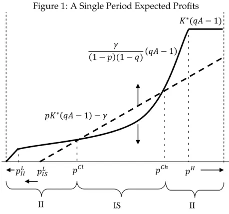
Figure 1 shows the ex-ante expected profits, net of the expected value of land, under these two information regimes, for each possible p. From comparing these profits we obtain the values ofpfor which the firm prefers to borrow with an information-insensitive loan (II) or with an information-sensitive loan (IS).
Figure 1: A Single Period Expected Profits
II IS II 𝑝𝐼𝐼𝐿 𝑝𝐼𝑆𝐿 𝑝𝐶𝑙 𝑝𝐶ℎ 𝑝𝐻 𝐾∗(𝑞𝐴 −1) 𝑝𝐾∗(𝑞𝐴 −1)− 𝛾 𝛾 (1− 𝑝)(1− 𝑞)(𝑞𝐴 −1)
The cutoffs highlighted in Figure 1 are determined in the following way:
1. The cutoffpH is the belief that generates the first kink of information-insensitive profits, below which firms have to reduce borrowing to prevent information
production:
pH = 1− γ
K∗(1−q). (3)
2. The cutoffpL
II comes from the second kink of information-insensitive profits,7
pLII = 1 2 − s 1 4 − γ C(1−q). (4) 3. The cutoffpL
IS comes from the kink of information-sensitive profits
pLIS = γ
K∗(qA−1). (5)
4. CutoffspChandpClare obtained from equalizing the profit functions of
information-sensitive and ininformation-sensitive loans and solving the quadratic equation
γ = pK∗− γ (1−p)(1−q) (qA−1). (6)
There are only three regions of financing. Information-insensitive loans are chosen for collateral with high and low values of p. Information-sensitive loans are chosen for collateral with intermediate values ofp.
To understand how these regions depend on the information cost γ, the five arrows in the figure show how the different cutoffs and functions move as we reduce γ. If information is free (γ = 0), all collateral is information-sensitive (i.e., the IS region is
p ∈ [0,1]). Contrarily, as γ increases, the two cutoffs pCh and pCl converge and the
IS region shrinks until it disappears (i.e., the II region is p ∈ [0,1]) when γ is large enough (specifically, whenγ > KC∗(C−K∗)).
7The positive root for the solution ofpC =γ/(1−p)(1−q)is irrelevant since it is greater thanpH,
and then it is not binding given all firms with a collateral that is good with probability p > pH can
borrow the optimal level of capitalK∗without triggering information acquisition.
Then, borrowing for each beliefp, conditional onγis, K(p|γ) = K∗ if pH < p γ (1−p)(1−q) ifp Ch < p < pH pK∗−(qAγ−1) ifpCl< p < pCh γ (1−p)(1−q) ifp L II < p < pCl pC if p < pL II
2.3
The Choice of Collateral
Collateral is heterogenous in two dimensions, the expected value of land p and the cost of information acquisition γ. If firms can freely choose the cost to monitoring collateralγ, then it is helpful to think about which collateral is more likely to be used when borrowing.
Above we derived borrowing for differentpand fixedγ. Similarly, we can derive bor-rowing for differentγ and fixedp. The next Proposition summarizes their properties.
Proposition 1 Effects ofpandγon borrowing.
Consider collateral characterized by the pair(p, γ). The reaction of borrowers to these variables depends on the financial constraint and information sensitiveness.
1. Fixγ.
(a) No financial constraint: Borrowing is independent ofp. (b) Information-sensitive regime: Borrowing is increasing inp. (c) Information-insensitive regime: Borrowing is increasing inp.
2. Fixp.
(a) No financial constraint: Borrowing is independent ofγ. (b) Information-sensitive regime: Borrowing is decreasing inγ.
(c) Information-insensitive regime: Borrowing is increasing in γ if higher than pC
and independent ofγifpC.
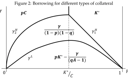
Figure 2: Borrowing for different types of collateral 𝑲∗ 𝒑𝑪 𝒑𝑲∗− 𝜸 (𝒒𝑨 − 𝟏) 𝜸 (𝟏 − 𝒑)(𝟏 − 𝒒) 𝑝 𝛾 0 𝐾∗ 1 𝐶 � 𝛾1𝐻 𝛾2𝐻 𝛾𝐿
The proof is in Appendix A.1. Figure 2 shows these regions and the borrowing pos-sibilities for all combinations(p, γ).
If it were possible for borrowers to choose the difficulty for lenders to monitor collat-eral with beliefp, then they would setγ > γH
1 (p)for thatp, such thatp > pH(γ)and the borrowing isK∗, without information acquisition.
This analysis suggests that, endogenously, an economy would be biased towards us-ing collateral with relatively highpand relatively highγ. Agents in an economy with increasing needs for collateral will first start using collateral that is perceived to be of high quality, and later move towards using collateral of worse quality but mak-ing information acquisition difficult and expensive. Even when outside the scope of our paper, this framework can shed light in rationalizing security design and the complexity of modern financial instruments.
2.4
Aggregation
The expected consumption of a household that lends to a firm with land that is good with probabilitypisK−K(p) +E(repay|p). The expected consumption of a firm that borrows using land that is good with probabilityp isE(K0|p)−E(repay|p). Aggre-gate consumption is the sum of the consumption of all households and firms. Since
E(K0|p) = qAK(p)
Wt=K+
Z 1 0
K(p)(qA−1)f(p)dp
where f(p) is the distribution of beliefs about collateral types in the economy and
K(p)is monotonically increasing inp.
In the unconstrained first best (the case of verifiable output, for example) all firms borrow and operate withK∗, regardless of beliefspabout the collateral. This implies that the unconstrained first best aggregate consumption is
W∗ =K+K∗(qA−1).
Since collateral with relatively lowpis not able to sustain loans ofK∗, the deviation of consumption from the unconstrained first best critically depends on the distribution of beliefs p in the economy. When this distribution is biased towards low percep-tions about collateral values, financial constraints hinder the productive capacity of the economy. This distribution also introduces heterogeneity in production, purely given by heterogeneity in collateral and financial constraints, not by heterogeneity in technological possibilities.
In the next section we study how this distribution of p endogenously evolves over time, and how that affects the dynamics of aggregate production and consumption.
3
Dynamics
In this section we nest the previous analysis for a single period in an overlapping generations economy. The purpose is to study the evolution of the distribution of col-lateral beliefs that determines the level of production in the economy at every period. We assume that each unit of land changes quality over time, mean reverting towards the average quality of collateral in the economy, and we study how endogenous in-formation acquisition shapes the distribution of beliefs over time. First, we study the case without aggregate shocks to collateral, in which the average quality of collateral in the economy does not change, and discuss the effects of endogenous information production on the dynamics of credit. Then, we introduce aggregate shocks that re-duce the average quality of collateral in the economy and generate crises, and study the effects of endogenous information on the size of crises and the speed of recoveries.
3.1
Extended Setting
We assume an overlapping generation structure, with a mass 1 of risk neutral indi-viduals who live for two periods. These indiindi-viduals are born as households (when
”young”), with endowment of numeraireK¯ but no managerial skills, and then become firms when”old”, with managerial skillsL∗, but no numeraire to use in production. We assume the numeraire is non-storable and land is storable until the moment its intrinsic value (eitherCor0) is extracted. Since land can be transferred across genera-tions, firms hold land. When young, individuals use their endowment of non-storable numeraire to buy land, which is useful as collateral when old to borrow productive numeraire.
This is reminiscent of the role of fiat money in overlapping generations, with the critical difference being that land is intrinsically valuable, is subject to imperfect in-formation about its quality, and is used as collateral. As in those models, we have multiple equilibrium based on multiple paths of rational expectations of land prices. In Appendix A.3 we discuss this multiplicity of prices.
We impose restrictions that simplify the price of a unit of land with belief p, to in-clude just the expected intrinsic valuepC, and not its potential role as collateral. This equilibrium has the advantage of isolating the dynamics generated by information acquisition from the better understood dynamics generated by beliefs about future prices of collateral. Still, the information dynamics we focus on in this equilibrium remains in other equilibria, when the price of land is increasing inp.
The first of these restrictions is that information can be produced only at the begin-ning of the period, not at the end. This assumption simplifies the price of land and also justifies that firms prefer to post land as collateral rather than sell land at the risk of information production. The second assumption is that each seller of land (each old individual at the end of the period) matches with a unique buyer who has the bargaining power (makes a take-it-or-leave-it offer). This implies that sellers will be indifferent between selling the unit of land atpC or consumingpC in expectation.8 Under these assumptions, the single period analysis repeats over time. The only
8It is simple to modify the model to sustain this assumption. For example, if a small fraction of
households inherit an endowment of new land, there will be more firms selling land than households buying land. Since sellers who do not sell just deplete their unsold land, the mass of land sustaining production in the economy is invariant. In Appendix A.3 we relax this assumption.
changing state variable linking periods is the distribution of beliefs about collateral. This evolving distribution may generate credit booms but also credit crises. Hence, there is a critical difference with models where credit booms and crises arise from bubbles in the price of each unit of collateral, and this paper in which the price of each unit of collateral is its fundamental value, and credit booms and crashes arise from the units of land that can be used as collateral in the economy.
3.2
No Aggregate Shocks
We impose a specific process of idiosyncratic mean reverting shocks that are useful in characterizing analytically the dynamic effects of information production on aggre-gate consumption. First, we assume idiosyncratic shocks are observable, but not their realization, unless information is produced. Second, we assume that the probability land faces an idiosyncratic shock is independent of its type. Finally, we assume the probability that land becomes good, conditional on having an idiosyncratic shock, is also independent of its type. These assumptions are just imposed to simplify the exposition. The main results of the paper are robust to different processes, as long as there is mean reversion of collateral in the economy.
Specifically, we assume that initially (at period 0) there is perfect information about which collateral is good and which is bad. In every period, with probabilityλthe true quality of each unit of land remains unchanged and with probability(1−λ)there is an idiosyncratic shock that changes its type. In this last case, land becomes good with a probabilitypˆ, independent of its current type. Even when the shock is observable, the realization of the new quality is not, unless a certain amount of the numeraire goodγ is used to learn about it.9
In this simple stochastic process for idiosyncratic shocks, and in the absence of ag-gregate shocks to pˆ, this distribution has a three-point support: 0,pˆand1. The next proposition shows the evolution of aggregate consumption depends on the borrow-ing ofpˆ, which can be either in the information sensitive or insensitive region.
Proposition 2 Evolution of aggregate consumption in the absence of aggregate shocks.
9To guarantee that all land is traded, buyers of good collateral should be willing to payCfor a good
land even when facing the probability that land may become bad next period, with probability(1−λ). The sufficient condition is given by enough persistence of collateral such thatλK∗(qA−1)>(1−λ)C. Furthermore they should have enough resources to buy good collateral, thenK > C¯ .
Assume there is perfect information about land types in the initial period. If pˆ is in the information-sensitive region (pˆ∈[pCl, pCh]), consumption is constant over time and is lower than the unconstrained first best. If pˆis in the information-insensitive region, consumption grows over time if p >ˆ pˆ∗h or p <ˆ pˆ∗l, where pˆ∗l and pˆ∗h are the solutions to the quadratic equation (1−ˆp∗γ)(1−q) = ˆp
∗K∗
.
Proof
1. pˆis information-sensitive (pˆ∈[pCl, pCh])
In this case, information about the fraction(1−λ)of collateral that gets an idiosyn-cratic shock is reacquired every period t. Then f(1) = λpˆ, f(ˆp) = (1 − λ) and
f(0) =λ(1−pˆ). ConsideringK(0) = 0,
WtIS = ¯K+ [λpKˆ (1) + (1−λ)K(ˆp)] (qA−1). (7)
Aggregate consumptionWIS
t does not depend ont; it is constant at the level at which
information is reacquired every period.
2. pˆis information-insensitive (p > pˆ Chorp < pˆ Cl)
Information on collateral that suffers an idiosyncratic shock is not reacquired and at periodt,f(1) =λtpˆ,f(ˆp) = (1−λt)andf(0) =λt(1−pˆ). SinceK(0) = 0,
WtII = ¯K+λtpKˆ (1) + (1−λt)K(ˆp)(qA−1). (8)
Since WII
0 = ¯K + ˆpK(1)(qA−1) and limt→∞WtII = ¯K +K(ˆp)(qA−1), the
evolu-tion of aggregate consumpevolu-tion depends on pˆ. A credit boom ensues and aggregate consumption grows over time, wheneverK(ˆp)>pKˆ (1), or
γ
(1−pˆ∗)(1−q) >pˆ ∗
K∗.
Q.E.D. This result is particularly important if the economy has collateral such thatp > pˆ H. In
this case consumption grows over time towards the unconstrained first best. When ˆ
p is high enough, the economy has an average enough collateral to sustain on pro-duction at the optimal scale. As information is lost in the economy good collateral implicitly subsidizes bad collateral and with time all firms are able to produce.
3.3
Aggregate Shocks
Now we introduce negative aggregate shocks that transform a fraction(1−η)of good collateral into bad collateral. As with idiosyncratic shocks, the aggregate shock is observable, but which good collateral changes type is not. When the shock hits, there is a downward revision of beliefs for all collateral. That is, after the shock, collateral with belief p = 1, gets revised downwards top0 = ηand collateral with belief p = ˆp
gets revised downwards top0 =ηpˆ.
Based on the discussion about the endogenous choice of collateral, which justifies that collateral would be constructed to maximize borrowing and prevent informa-tion acquisiinforma-tion, we focus on the case where, prior to the negative aggregate shock, the average quality of collateral is good enough such that there are no financial con-straints (that is,p > pˆ H).
In the next proposition we show that the longer the economy does not face a negative aggregate shock, the larger the consumption loss when such a shock does occur.
Proposition 3 The larger the boom and the shock, the larger the crisis.
Assumep > pˆ H and a negative aggregate shockηin periodt. The reduction in consumption
∆(t|η)≡Wt−Wt|ηis non-decreasing in shock sizeηand non -decreasing in the timetelapsed
previously without a shock.
Proof Assume a negative aggregate shock of size η. Since we assume p > pˆ H, the
average collateral does not induce information. Aggregate consumption before the shock is given by equation (8). Aggregate consumption after the shock is:
Wt|η = ¯K+
λtpKˆ (η) + (1−λt)K(ηpˆ)
(qA−1).
Defining the reduction in aggregate consumption as∆(t|η) =Wt−Wt|η
∆(t|η) = [λtpˆ[K(1)−K(η)] + (1−λt)[K(ˆp)−K(ηpˆ)]](qA−1).
That ∆(t|η)is non-decreasing in ηis straightforward. That ∆(t|η)is non-decreasing intfollows from
ˆ
p[K(1)−K(η)]≤[K(ˆp)−K(ηpˆ)] 18
which holds becauseK(ˆp) = K(1)(by assumptionp > pˆ H) andK(p)is monotonically
decreasing inp. Q.E.D.
The intuition for this proposition is the following. Pooling implies that bad collateral is confused with good collateral. This allows for a credit boom because firms with bad collateral get credit that they would not obtain otherwise. Firms with good col-lateral effectively subsidize firms with bad colcol-lateral since good colcol-lateral still gets the optimal leverage, while bad collateral is able to leverage more.
However, pooling also implies that good collateral is confused with bad collateral. This puts good collateral in a weaker position in the event of negative aggregate shocks. Without pooling, a negative shock reduces the belief that collateral is good fromp= 1top0 =η. With pooling, a negative shock reduces the belief that collateral is good from p = ˆp to p0 = ηpˆ. Good collateral gets the same credit regardless of having beliefsp= 1orp= ˆp. However credit may be very different underp=ηand
p =ηpˆ. Furthermore, after a negative shock to collateral, either a high amount of the numeraire is used to produce information, or borrowing is excessively restricted to avoid such information production.
If we define”fragility” as the probability aggregate consumption declines more than a certain value, then the next corollary immediately follows from Proposition 3.
Corollary 1 Given a structure of negative aggregate shocks, the fragility of an economy
increases with the number of periods the debt in the economy has been informationally-insensitive, and henceincreaseswith the fraction of collateral that is of unknown quality.
In the next proposition we show that information acquisition speeds up recoveries.
Proposition 4 Information and recoveries.
Assume p > pˆ H and a negative aggregate shock η in period t. The recovery is faster when information is generated after the shock when ηp < ηˆ pˆ≡ 1
2 + q 1 4 − γ K∗(1−q), wherepCh <
ηp < pˆ H. That is,WtIS+1 > WtII+1 for allηp < ηˆ pˆandWtIS+1 ≤WtII+1 otherwise.
ProofIf the negative shock happens in periodt, the belief distribution isf(η) = λtpˆ,
f(ηpˆ) = (1−λt)andf(0) =λt(1−pˆ).
In period t + 1, if information is acquired (IS case), after idiosyncratic shocks are realized, the belief distribution isfIS(1) =ληpˆ(1−λt),fIS(η) =λt+1pˆ,fIS(ˆp) = (1−λ),
fIS(0) = λ[(1 −λtpˆ)−ηpˆ(1−λt)]. Hence, aggregate consumption at t+ 1 in theIS
scenario is,
WtIS+1 =K+ [ληpˆ(1−λt)K∗+λt+1pKˆ (η) + (1−λ)K(ˆp)](qA−1). (9)
In periodt+ 1, if information is not acquired (II case), after idiosyncratic shocks are realized, the belief distribution isfII(η) =λt+1pˆ,fII(ˆp) = (1−λ),fII(ηpˆ) =λ(1−λt),
fII(0) =λt+1(1−pˆ). Hence, aggregate consumption att+ 1in theII scenario is,
WtII+1 =K+ [λt+1pKˆ (η) +λ(1−λt)K(ηpˆ) + (1−λ)K(ˆp)](qA−1). (10)
Taking the difference between aggregate consumption att+1between the two regimes
WtIS+1−WtII+1 =λ(1−λt)(qA−1)[ηpKˆ ∗−K(ηpˆ)]. (11) This expression is non-negative for all ηpKˆ ∗ ≥ K(ηpˆ), or alternatively, for all ηp <ˆ
ηpˆ≡ 1 2 + q 1 4 − γ K∗(1−q). From equation (6),pCh < ηp < pˆ H. Q.E.D. The intuition for this proposition is the following. When information is acquired after a negative shock, not only are a lot of resources spent in acquiring information but also only a fraction ηpˆof collateral can sustain the maximum borrowingK∗. When information is not acquired after a negative shock, collateral that remains with belief
ηpˆwill restrict credit in the following periods, until beliefs move back to pˆ. This is equivalent to restricting credit proportional to monitoring costs in subsequent peri-ods. Not producing information causes a kind of debt overhang going forward. The proposition generates the following Corollary.
Corollary 2 There exists a range of negative aggregate shocks (ηsuch thatηpˆ∈[pCh, ηpˆ]) in which agents do not acquire information, but recovery would be faster if they did.
The next Proposition describes the evolution of the standard deviation of beliefs in the economy during a credit boom. This proposition will be the basis of the empirical analysis in Section 5.
Proposition 5 During a credit boom, the standard deviation of beliefs declines.
ProofAssume at period0that the belief distribution isf(0) = 1−pˆandf(1) = ˆp. The original variance of beliefs is
V ar0(p) = ˆp2(1−pˆ) + (1−pˆ)2pˆ= ˆp(1−pˆ).
At periodt, during a credit boom, the belief distribution isf(0) = λt(1−pˆ), f(ˆp) = 1−λtandf(1) =λtpˆ. Then, at periodtthe variance of beliefs is
V art(p|II) = λt[ˆp2(1−pˆ) + (1−pˆ)2pˆ] =λtpˆ(1−pˆ),
decreasing in the length of the boomt. Q.E.D.
Finally, the next Proposition describes the evolution of the standard deviation of be-liefs in the economy during a crisis.
Proposition 6 The increase in the dispersion of beliefs after a crisis is larger after a longer boom.
For a negative aggregate shockηthat triggers information about collateral with beliefηpˆ, the increase of the standard deviation of beliefs is increasing in the length of the credit boomt.
ProofAssume a shockηat periodtthat triggers information acquisition about collat-eral with beliefηpˆ. If the shock is”small”(η > pCh), there is no information acquisition about collateralknown to be good before the shock. If the shock is”large”(η < pCh), there is information acquisition about collateralknown to be good before the shock. Now we study these two cases when the shock arises after a credit boom of lengtht. 1. η > pCh. The distribution of beliefs in case information is generated is given by
f(0) =λt(1−pˆ) + (1−λt)(1−ηpˆ),f(η) =λtpˆandf(1) = (1−λt)ηpˆ. Then, at periodt
the variance of beliefs with information production is
V art(p|IS) = λtpˆ(1−pˆ)η2+ (1−λt)ηpˆ(1−ηpˆ),
Then
V art(p|IS)−V art(p|II) = (1−λt)ηpˆ(1−ηpˆ)−λtpˆ(1−pˆ)(1−η2),
increasing in the length of the boomt.
2. η < pCh. The distribution of beliefs in case information is produced is given by
f(0) =λt(1−pˆ) + (1−λt(1−pˆ))(1−ηpˆ), andf(1) = (1−λt(1−pˆ))ηpˆ. Then, at period
tthe variance of beliefs with information production is
V art(p|IS) =λtpˆ(1−pˆ)η2pˆ+ (1−λt(1−pˆ))ηpˆ(1−ηpˆ),
Then
V art(p|IS)−V art(p|II) = (1−λt(1−pˆ))ηpˆ(1−ηpˆ)−λtpˆ(1−pˆ)(1−η2pˆ),
also increasing in the length of the boomt.
The change in the variance of beliefs also depends on the size of the shock. For very large shocks (η → 0) the variance can decline. This decline is lower the larger ist.
Q.E.D.
3.4
Numerical Illustration
In this subsection we illustrate our dynamic results with a numerical example. We assume idiosyncratic shocks happen with probability(1−λ) = 0.1, in which case the collateral becomes good with probabilitypˆ= 0.92. Other parameters areq= 0.6,A= 3(investment is efficient and generates a return of 80%), K¯ = 10, L∗ = K∗ = 7 (the endowment is large enough to allow for optimal investment),C = 15andγ = 0.35. Given these parameters we can obtain the relevant cutoffs for our analysis. Specif-ically, pH = 0.88, pL
II = 0.06and the region of beliefs p ∈ [0.22,0.84] is information
sensitive. Figure 3 plots the ex-ante expected profits with information sensitive and insensitive debt, and the respective cutoffs.
Using these cutoffs in each period, we simulate the model for 100 periods. At period 0 there is perfect information about the true quality of all collateral in the economy. Over time, idiosyncratic shocks make information to vanish unless it is replenished. The dynamics of consumption arises from the dynamics of belief distribution.
We introduce a negative aggregate shock that transforms a fraction(1−η)of good col-lateral into bad colcol-lateral in periods 5 and 50. We also introduce a positive aggregate
Figure 3: Expected Profits and Cutoffs 0 0.2 0.4 0.6 0.8 1 0 1 2 3 4 5 6 Beliefs Expected Profits E() II E() IS
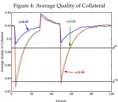
shock that transforms a fraction0.25of bad collateral into good collateral in period 30. We compute the dynamic reaction of consumption in the economy for different sizes of negative aggregate shocks,η = 0.97, η = 0.91and η = 0.90. We will see that small differences in the size of a negative shock can have large dynamic consequences. Figure 4 shows the evolution of the average quality of collateral for the three negative and the positive aggregate shocks we assume. Aggregate shocks have a temporary effect on the quality of collateral because mean reversion makes average quality con-verge back to pˆ= 0.92. We choose the size of the negative aggregate shocks to guar-antee thatηpˆis abovepH whenη= 0.97, is betweenpCh andpH whenη = 0.91and is less thanpChwhenη= 0.90.
Figure 5 shows the evolution of aggregate consumption for the three negative aggre-gate shocks. A couple of features are worth noting. First, if η = 0.97, the aggregate shock is small enough such that it does not constrain borrowing and does not modify the evolution of consumption. Second, the positive shock does not affect the evolu-tion of consumpevolu-tion either. Since p > pˆ H a further improvement in average beliefs does not further relax financial constraints.
As proved in Proposition 3, ifη= 0.91orη= 0.90, the reduction in consumption from the shock in period 50, when the credit boom is mature and information is scarce, is larger than the reduction in consumption when the shock happens in period 5. Fur-thermore, consumption drops to a lower level in period 50 than in period 5. The
Figure 4: Average Quality of Collateral 0 20 40 60 80 100 0.82 0.84 0.86 0.88 0.9 0.92 0.94 Periods
Average Quality of Collateral
=0.97 =0.91
=0.90
pH
pCh
reason is that the shock reduces financing for a larger fraction of collateral when in-formation has vanished over time. As proved in Proposition 4, a shockη = 0.91does not trigger information production, but a shockη = 0.90does. Even when these two shocks generate consumption crashes of similar magnitude, recovery is faster when the shock is slightly larger and information is replenished.
Figure 5: Welfare 0 20 40 60 80 100 13.8 14 14.2 14.4 14.6 14.8 15 15.2 15.4 15.6 15.8 Periods Aggregate Consumption =0.97 =0.90 =0.91 Always produce information about idiosyncratic shocks
Finally, Figure 6 shows the evolution of the dispersion of beliefs about the collateral, a measure of available information in the economy. As proved in Proposition 5, a
credit boom is correlated with a reduction in the dispersion of beliefs. As proved in Proposition 6, given that after many periods without a shock most collateral looks the same, the information acquisition triggered by a shockη= 0.90generates a larger increase in dispersion in period 50 than in period 5.
Figure 6: Standard Deviation of Distribution of Beliefs
0 20 40 60 80 100 0 0.05 0.1 0.15 0.2 0.25 0.3 0.35 0.4 Periods
Standard Deviation of Beliefs
=0.97
=0.91 =0.90
3.5
Discussion
Here we briefly discuss some issues that may have occurred to the reader. We have motivated the model’s structure based on appealing to the micro foundations of Dang, Gorton, and Holmstr ¨om (2011), where the best transaction medium is short-term debt. In our model, as it stands, the land could simply be sold by the old gen-eration (the borrowers) to the young gengen-eration (the lenders). This is because we did not include a need for the young to have a transactions medium to use to shop during their first period, and before the output is realized. If there was such a market, the young would need to use the collateralized claims on the firm as ”money.” That is the idea of short-term debt as money. For simplicity we did not include such a market. In the model the firms are also uninformed about their own collateral quality. Like the households they do not produce information every period because it is costly. We view this as realistic. There may be other reasons to think that firms could differ in ways which are unobservable to the households, so that there are firm types. This
is a well-studied setting and we do not include it here. The main reason for this omission is that we have abstracted from the financial intermediaries, which would be screening firms and issuing liabilities to the households for use as money. This is a subject for future research.
What about other reasons for producing information? We have eliminated all other possible model embellishments and complications in order to focus attention on the endogenous dynamics of information production in the economy with regard to short-term debt. Clearly, however, there are other reasons why information should be pro-duced. For example, firms might want to produce information in order to learn their best investment opportunities. The interaction of such information production with the possible production of information about the firm’s collateral potentially raises interesting issues. For example, producing information about firms not only induces more efficient investment but also leads to less borrowing in expectation. This is also a subject of future research.
Finally, it is worth noting the differences between our model and a recent literature in which credit constraints or other frictions generate ”over borrowing.” In some of these settings private agents do not internalize the effects of their own leverage in depressing collateral prices in case of shocks that trigger fire sales. Since a shock is an exogenous unlucky event, the policy implications are clear: there should be less borrowing. Examples of this literature would include Lorenzoni (2008), Mendoza (2010) and Bianchi (2011). In contrast to these settings, there is nothing necessarily bad about leverage in our model, compared to these models. First, leverage always relaxes endogenous credit constraints. Second, fire sales are not an issue. In our setting the efficient outcome may be fragility.
4
Policy Implications
In this section we discuss optimal information production when a planner cares about the discounted consumption of all generations and faces the same information restric-tions and costs that households and firms. Welfare is measured by
Ut=Et ∞ X τ=t βτ−tWt. 26
First, we study the economy without aggregate shocks, and show that a planner would like to produce information for a wider range of collateral pthan short-lived agents. Then, we study the economy with negative aggregate shocks, and show that a planner is more likely to trigger information acquisition than decentralized agents. However, when expected shocks are not very large or likely, it may be optimal for the planner to avoid information production, riding the credit boom even when facing the possibility of collapses.
4.1
Ex-Ante Policies in the Absence of Aggregate Shocks
The next Proposition shows that, whenβ > 0, the planner wants to acquire informa-tion for a wider range of beliefsp.
Proposition 7 The planner’s optimal range of information-sensitive beliefs is wider than the the decentralized range of information-sensitive beliefs.
ProofDenote the expected discounted consumption sustained by a unit of collateral with beliefpif producing information (IS) as
VIS(p) = pK∗(qA−1)−γ+β[λ(pV(1) + (1−p)V(0)) + (1−λ)V(ˆp)] +pC
and expected discounted consumption if not producing information (II) as
VII(p) = K(p)(qA−1) +β[λV(p) + (1−λ)V(ˆp)] +pC
We can solve for
VIS(p) = pK ∗(qA−1) 1−βλ −γ+Z(p,pˆ) and VII(p) = K(p)(qA−1) 1−βλ +Z(p,pˆ), whereZ(p,pˆ) =βhλβ1−(1−βλλ) + (1−λ)iV(ˆp) +pC.
The planner decides to acquire information ifVIS(p)> VII(p), or
γ(1−βλ)<[pK∗−K(p)](qA−1),
while, as shown in equation (6), individuals decide to acquire information when
γ <[pK∗−K(p)](qA−1),
which effectively means the decision rule for the planner is the same that the decision rule for decentralized agents, but with β > 0for the planner and β = 0for agents.
Q.E.D.
The cost of information is effectively lower for the planner, since acquiring informa-tion has the addiinforma-tional gain of enjoying more borrowing in the future if the collateral is found to be good. The difference between the planner and the agents widens with the government discounting (β) and with the probability that the collateral remains unchanged (λ).
The planner can align incentives easily by subsidizing information production by an fractionβλfrom lump sum taxes on individuals, such that, after the subsidy, the cost of information production agents face is effectivelyγ(1−βλ).
4.2
Ex-Ante Policies in the Presence of Aggregate Shocks
In this section we assume that the planner assigns a probability µ that a negative shock occurs next period. The next two propositions summarize how the incentives to acquire information change with the probability and the size of aggregate shocks.
Proposition 8 Incentives to acquire information in the presence of aggregate shocks increases with the probability of the shockµifp[K∗−K(η)]≤[K(p)−K(ηp)], and decreases otherwise.
ProofWithout loss of generality we assume the negative shock can happen only once. Expected discounted consumption sustained by a unit of collateral with belief p if information is produced (IS) is
VIS(p) = pK∗(qA−1) +β[(1−µ)[λ(pV(1) + (1−p)V(0)) + (1−λ)V(ˆp) +µ[λ(pV(η) + (1−p)V(0)) + (1−λ)V(ηpˆ)] +pC,
and if information is not produced (II) is
VII(p) =K(p)(qA−1) +β[(1−µ)[λV(p) + (1−λ)V(ˆp) +µ[λV(ηp) + (1−λ)V(ηpˆ)] +pC.
We can solve for VIS(p) = pK ∗(qA−1) 1−βλ − βλµ 1−βλp[K ∗− K(η)](qA−1) +Z(p,pˆ) and VII(p) = K(p)(qA−1) 1−βλ −γ− βλµ 1−βλ[K(p)−K(ηp)](qA−1) +Z(p,pˆ).
Naturally, the expectation of aggregate shocks reduces expected consumption in both situations. The effect on information production depends on which one drops more. The Proposition arises straightforwardly from comparingVIS(p)andVII(p). Q.E.D.
To build intuition, assume η is such thatK(ηp) < K(p) and K(η) = K∗, for exam-ple if the shock is small and p = pH. In this case, the aggregate shock, regardless of its probability, does not affect the expected discounted consumption of acquiring information, but reduces the expected discounted consumption of not acquiring in-formation. In this case, producing information relaxes the borrowing constraint in case of a future negative shock, and when that shock is more likely, there are more incentives to acquire information.
Proposition 9 Incentives to acquire information in the presence of aggregate shocks increases with the size of the shock (decreases withη) if ∂K∂η(ηp) ≤p∂K∂η(η), and decreases otherwise.
Proof Define DV(p) = VIS(p)− VII(p), which measures the incentives to acquire information. Taking derivatives with respect to η, incentives to acquire information increase with the size of the shock (decrease withη) is
∂DV(η|p) ∂η = βλµ 1−βλ ∂K(ηp) ∂η −p ∂K(η) ∂η ≤0. Q.E.D.
The effect is clearly non-monotonic in the size of the shock. For example, at the ex-treme of very large shocks (η= 0), in which all collateral becomes bad, the incentives to produce information in fact decline, since the condition in that case becomes
γ 1−βλ
1−βλµ < pK
∗−
K(p),
increasing the effective cost of acquiring information. In this extreme case, the plan-ner still wants to acquire more information than decentralized agents, but less than in the absence of an aggregate shock (since(1−βλ)≤ 1−1−βλµβλ ≤1).
The previous two propositions show there are levels ofpfor which, even in the pres-ence of a potential future negative shock the planner prefers not producing infor-mation, maintaining a high level of current output rather than avoiding a potential reduction in future output. This result is summarized in the following Corollary.
Corollary 3 The possibility of a negative aggregate shock does not necessarily justify acquir-ing information, and reducacquir-ing current output to insure against potential future crises.
This corollary suggests that there are conditions under which it is efficient to accept potential reductions in future consumption in order to obtain guaranteed increases in current consumption. This result is consistent with the findings of Ranciere, Tor-nell, and Westermann (2008) who show that ”high growth paths are associated with the undertaking of systemic risk and with the occurrence of occasional crises.”
4.3
Ex-Post Policies
Now we study ex-post policies, conditional on a realized aggregate shock. Naturally these policies affect the results in the previous section, since if they are effective in helping the economy recover, they render ex-ante information acquisition to relax borrowing constraints less important in the presence of aggregate shocks.
We consider policies that are intended to boost the expected quality of collateral after a negative aggregate shock. The effectiveness of such a policy depends on how fast the government is able to react to the negative shock, for example guaranteeing the quality of the collateral. This policy manifests itself as a positive aggregate shock in which a fraction α of bad collateral becomes good one period after the negative aggregate shock, for example collateral guarantees by the government.
The next Proposition shows that, if there is a positive aggregate shock after a negative aggregate shock that takes the average collateralηpˆto a new higher level above pH,
the recovery from the negative shock is faster if at the same time the government prevents information production as a response to the negative shock.
Proposition 10 Ex-post policies are more effective if information acquisition is avoided. Assume a negative aggregate shock η that induces information acquisition (this is ηpˆ ∈
[pCl, pCh]), immediately followed by a positivepolicyof sizeαthat makes firms able to borrow
K∗ (this isp0 =ηpˆ+α(1−ηpˆ)> pH). This policy is more effective in speeding up recovery
if information werenotacquired. More specifically∆II >∆IS (where∆II ≡WII
t+1|α−W II t+1 and∆IS ≡WIS t+1|α−W IS t+1).
The proof is in Appendix A.2. The intuition relies on the speed of information re-covery. Assume all collateral has the same belief and an aggregate negative shock induces information that sorts out the quality of collateral. In this case, a successful policy that improves average quality does not have a big impact. It does not increase borrowing for the good collateral and only helps marginally the bad collateral. But, if the aggregate negative shock does not induce information production, then a suc-cessful policy that improves average quality increases the borrowing both of the good and the bad collateral types.
Figure 7 introduces a policy that boosts the average quality of collateral in the numer-ical illustration of the previous section. Specifnumer-ically it assumes a policy α = 0.25in period 51, right after a negative shock. As can be seen, this policy is more effective in speeding up recovery when the negative shock did not induce information.
Figure 7: Effectiveness of Collateral Policy
0 20 40 60 80 100 13.8 14 14.2 14.4 14.6 14.8 15 15.2 15.4 15.6 15.8 Periods Aggregate Consumption =0.97 =0.90 Always produce information about idiosyncratic shocks =0.91
This implies that, if the planner has access to a policy to deal with a crises, such as guaranteeing collateral use, that policy is more effective if the original shock does not
induce information acquisition in the economy. How can the government prevent in-formation acquisition after a crisis? Possibly introducing a lending facility, financed through household taxation, that covers the difference between the optimal borrow-ing and the level of borrowborrow-ing that in equilibrium would induce information.
5
Some Empirical Evidence
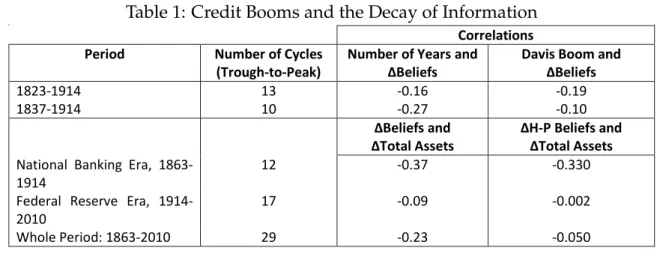
In this section we briefly examine the central prediction of the model, using U.S. his-torical data. The prediction from Proposition 5 is that during a credit boom the stan-dard deviation of beliefs declines. If information about collateral decays because no information is produced, then the standard deviation of beliefs is shrinking and lend-ing is increaslend-ing, leadlend-ing to higher output. The empirical strategy is to examine the correlation between the growth in credit creation (or output growth) and the change in the standard deviation of beliefs from the trough of a business cycle to the next business cycle peak.
There are a number of complications in implementing a test. We need to measure credit creation and beliefs. With regard to credit creation, there are no consistent time series that span a long period of U.S. history for credit creation, so we are forced to examine sub-periods and use less precise measures. We will look at banks’ total assets for most of the period, but to include the pre-Civil War period we will also look at industrial output. In the model, credit creation and output grow one-for-one. The bank total assets data are five or six times year from 1863-1923 and four times a year thereafter. The output data, however, are annual.
As for beliefs, we need a proxy for the distribution of perceived collateral quality. For simplicity the model is one in which firms have a constant expected marginal prod-uct of capital, but in terms of the empirical work, we want to imagine that firms have concave production technologies. In this case, expected returns can vary depending on the perceived quality of collateral. We proxy for beliefs with the standard devia-tion of the cross secdevia-tion of stock returns. The idea is that at each date we calculate the stock return over a given period (annual or monthly) and then for that date we calculate the standard deviation of the cross section of stock returns. We then have a time series of the cross section of stock returns. Over time, as information is decaying, the standard deviation of the cross section of stock returns should be shrinking.