Estimation of Credit and Default Spreads: An Application to CDO Valuation

Full text

(1)Estimation of Credit and Default Spreads: An Application to CDO Valuation. Jaesun Noh a ∗ Preliminary Draft November 27, 2002 a. ∗. CIBC, 161 Bay Street, 11th Floor, Toronto, ON M5J 2S8, Canada. Corresponding author. Tel.: 416-956-6060; Fax: 416-594-8528; E-mail: [email protected].. 1.

(2) Estimation of Credit and Default Spreads: An Application to CDO Valuation. Abstract Many securities are, to a certain extent, subject to credit risk in one way or another. Both the financial institutions and regulators are keen to have their credit risk exposures well managed. In order to fulfill their needs, the market for credit derivatives has become one of the fast growing securities markets in the last several years. In particular, the credit risk on a corporate balance sheet has become an important topic. Along with this growing importance of credit risk, the development of credit risk models has received much attention from both practitioners and academia. This paper addresses the impact of default rate modeling on the risk analysis and market valuation of credit derivatives products.. 2.

(3) I. Introduction Many securities are, to a certain extent, subject to credit risk in one way or another. Both the financial institutions and regulators are keen to have their credit risk exposures well managed. In order to fulfill their needs, the market for credit derivatives has become one of the fast growing securities markets in the last several years. In particular, the credit risk on a corporate balance sheet has become an important topic. Along with this growing importance of credit risk, the development of credit risk models has received much attention from both practitioners and academia. This paper addresses the impact of default rate modeling on the risk analysis and market valuation of credit derivatives products. Researchers attempt to model credit risk and valuation by using either one of the following two approaches: structural models or reduced form models. The first group, like KMV, mainly follows Merton (1974) by relating a firm’s credit risk to the variation of its asset and liability value through equity value. A default event occurs when its asset value is lower than certain threshold liability level. However, to implement this approach, firms’ assets need to be estimated, and the complex structure of payoffs of all the liabilities needs to be specified. For multi-factor models, given the complexity in modeling default as a first passage time event, it is difficult to obtain closed-form solutions. The second group, like Credit Metrics, Jarrow and Turnbull (1995), and Duffie and Singleton (1997), works on the credit migration and default probability based on the historical credit transition probability or market credit spreads without explicitly taking account of firms’ underlying asset values. Duffie and Singleton (1997) used the affine class of term structure models to capture both the cross-sectional and time-series properties. Delianedis and Geske (2000), Elton, Gruber et al (2001) described the discrepancy between the default spread and credit spread due to taxes, liquidity and market risk factors. For default rate modeling, there is little empirical evidence with which to differentiate the parameters guiding the dynamics of risk-neutral and actual default intensities. Jarrow, Lando, and Turnbull (1997) provided some methods for calibrating risk-neutral default intensities from ratings-based transition data and bond-yield spreads. Duffee (1998) provided some empirical estimates for the actual dynamics of risk-neutral default intensities for relatively low-risk corporate bond issuers, based on time-series data on corporate bonds. However, both studies provide hazard rate models for credit spreads not for default spreads. In this paper, we separately estimate the processes for default spreads and credit spreads combining the above two approaches. Since default process is an important factor in measuring credit risk and pricing credit derivatives, if there are big gaps between credit spreads and default spreads, it would make more sense to estimate default rate models using default spreads data rather than using credit spreads data. We find that default spreads account for only a small portion of credit spreads for investment grade firms and they display quite different volatility structure.. 3.

(4) In section II and III we describe a model for constructing credit spreads, default spreads and correlations. In section IV we describe the estimation procedures and section V shows how we model credit event generator. Section VI shows the estimation results and the impact of default correlation on the market value of Collateralized Debt Obligations (CDO).. 4.

(5) II. Credit and Default Spread Model In this section we describe an empirical approach to measure actual and risk neutral default probability. First we start with structural approach for default probability and bond pricing. Then we describe a parametric model for default process to compute credit and default spread using the market bond data and the default probability from the structural approach. A. Structural Approach Let Vt be the time t value of the firm i ’s assets and it follows, under the risk neutral measure,. dVi ,t = rVi ,t + σ i ,vVi ,t dZ i ,t. (1). where r is the risk-free interest rate. Under the actual measure, it can be written as follows:. dVi ,t = µ iVi ,t + σ i ,vVi ,t dZ i ,t. (2). where µ i = r + λiσ i ,v and λi is the price of risk. Merton (1974) modeled the option to default by considering the stock in a leveraged firm as a call option on the assets of the firm with an exercise price equal to the face value of the total debt:. S i = Vi N (k i + σ i ,v T − t ) − M − r (T −t ) eN (k i ). (3). where. ki =. ln(Vi / M i ) + ( µ i − 0.5σ i2,v )(T − t ). σ i ,ν T − t. and S i is the current market value of the stock, M i is the face value of debt. The probability that the firm will be insolvent and default on its debt obligation at date T is:. APDi = 1 − N (k i ). 5. (4).

(6) where N (⋅) is the cumulative normal distribution function. The risk neutral probability that the firm will be insolvent and default on its debt obligation at date T is1:.   (u − r ) RPDi = N  − k i + M Ri T − t  σM     (u − r ) = N  N −1 ( APDi ) + M Ri T − t  σM  . (5). Under the risk-averse assumption, the expected return on the firm must exceed the risk free rate. Since the actual and risk neutral distributions of the firm have the same variance and actual distribution must have a mean greater than the risk free rate, then the risk neutral distribution will have the larger default probability. To compute the above default probabilities, we need to estimate the asset value and asset volatility. In addition to equation (3), we need the following condition to estimate them 2:. σ S = σV (. V ∂V ) S ∂S. Using twelve months of daily data, we estimate the asset value and asset volatility iteratively until the asset volatility converges. This process is repeated every end of month. B. Reduced Form Approach Following Duffie and Singleton (1999), we describe the default-adjusted rate Rt as a sum of default-free interest rate rt and hazard rate g t multiplied by loss given default Lt , i.e., Rt = rt + g t Lt . Generally, g t and Lt are not separately identifiable. In this paper we assume constant Lt , equal to L . Since g t and Lt are not separately identifiable, the validity of this assumption will not affect the model performance in fitting the corporate bond prices. Moreover, an empirical study conducted by Skinner and Diaz (2000). 1. The firm i’s beta is. β i = Ri. σ i ,ν σM. where Ri is the correlation between the firm i’s return and the market. return. Hence, the equation (5) is expressed in terms of the market price of risk instead of the firm i’s price of risk. 2 Under certain conditions, the relationship can be expressed as follows (see CreditGrades):. σV = σ S. S . This implies that, for a stable asset volatility, the equity volatility increases with S+M. declining stock price consistent with volatility skew in equity option market.. 6. (6).

(7) suggests that allowing for time dependent variation in Lt is of secondary importance in pricing defaultable claims. We assume the default-free interest rate is defined as follows: rt = α r + s1t + s 2t ,. (7). and the two factors, s1t and s 2t , follow the CIR process: ds it = (κ irθ ir − κ ir s it )dt + σ ir s it dz it ds it = (κ irθ ir − (κ ir + λir ) sit )dt + σ ir s it dz it. (8). where (8) holds under the actual and risk neutral measure, respectively. The value of a default-free bond, G (t , T ) , for maturity T − t is given by T G (t , T ) = EtQ exp(− ∫ (rs )ds )   t = A1r (t , T ) A2 r (t , T ) exp(−α r (T − t ) − B1r (t , T ) s1t − B2 r (t , T ) s 2t ). (9). where, for i = 1 and 2,  2γ ir exp((air + γ ir )(T − t ) / 2)  Air (t , T ) =    (air + γ ir )(exp(γ ir (T − t )) − 1) + 2γ i . 2κ iθ i / σ i2.   2(exp(γ ir (T − t )) − 1) Bir (t , T ) =    (air + γ ir )(exp(γ ir (T − t )) − 1) + 2γ ir . air = k ir + λir. γ ir = air2 + 2σ ir2 .. (10). We also assume that the expected loss rate is defined as: g t L = (α h + ht + β 1 s1t + β 2 s 2t ) L. (11). where L = 1 − δ is the loss rate and δ is the recovery rate, and the hazard rate ht follows the CIR process:. 7.

(8) dht = (κ hθ h − κ h ht )dt + σ h ht dz ht. (12). dht = (κ hθ h − (κ h + λ h )ht )dt + σ h ht dz ht. (13). where (12) and (13) holds under the actual and risk neutral measure, respectively. The value of a risky zero-coupon bond, P (t , T ) , for maturity T − t , with constant recovery rate δ , is given by T P (t , T ) = EtQ exp(− ∫ (rs + g s L)ds )   t = Gh (t , T ){exp(− Lα h (T − t )) Ah (t , T ) exp(− Bh (t , T ) Lht )}. (14). where  2γ h exp((a h + γ h )(T − t ) / 2)  Ah (t , T ) =    (a h + γ h )(exp(γ h (T − t )) − 1) + 2γ h . 2κ hθ h / σ h2.   2(exp(γ h (T − t )) − 1) Bh (t , T ) =    (a h + γ h )(exp(γ h (T − t )) − 1) + 2γ h . a h = k h + λh. γ h = a h2 + 2σ h2 ,. (15). and Gh (t , T ) is G (t , T ) with β 1 s1t L and β 2 s 2t L instead of s1t and s 2t , respectively.. III. Default Intensity and Default Correlation. Using the default probability computed from the Merton model, we can price risky bond as follows: P (t , T ) = (1 − L) ⋅ G (t , T ) + L ⋅ G (t , T ) ⋅ (1 − CRPD(t , T )) ,. (16). Similar to Jones, Mason, and Rosenfeld (1984), risky bond can also be priced as follows: P(t , T ) = G (t , T )[ N (k ( M , T − t )). + VG (t , T ) −1 N (−k (δ , T − t )) + δ {N (k (δ , T − t )) − N (k ( M , T − t ))}]. 8. (17).

(9) where k ( x, τ ) =. ln(. V ) + (r − 0.5σ v2 )τ xM. σv τ. Once the time series of default spread or risky bond price with only default premium is estimated, similar to the hazard rate modeling in the above section, we can use a parsimonious Markov model for each obligor’s (or sector’s) default probabilities, while varying the correlation among different obligor’s default times. Duffie and Garleanu (1999) and Finger (2002) assumed that default times have default intensity processes ς i , which follow the CIR process described in equation (13) with parameters (κ i , θ i , σ i , λi ) i.e., dς it = (κ iθ i + δ i ς t − (κ i + λi )ς t )dt + σ i ς it dz it. (18). under the risk neutral measure and where ς t denotes the average default intensity. Alternatively, using the time series of risk neutral default probabilities, we can estimate the default intensities as follows:. ∆ς it = (κ iθ i + δ i ς t − (κ i + λi )ς t −1 )∆t + σ i ς it −1 * ∆t ε it. (19). where ς it (τ ) = − ln(1 − RPDit (τ )) . Then the correlation between the default intensities of firm i and j is computed as the correlation between ε it and ε jt over the sample period. We can also achieve the same goal using the time series of default spreads and the following relationship: e − sitτ = 1 − CRPDit (τ ) * L = 1 − {1 − (1 − RPDit (τ ))τ } * L where s it denotes default spreads3.. (20). IV. Estimation. Month-end prices of US Treasury bills, notes, bonds and corporate bonds are extracted from Bridge over the period of beginning July 1995 and ending February 2002. We restrict our sample to corporate bonds issued by U.S. firms. The bonds under consideration have semi-annual fixed rate coupons and principal at maturity. We also. 3. This implies that the default intensity is computed as:. 9. 1. ς it (τ ) = ( sit * τ + ln( L)) . τ.

(10) exclude bonds with call options, put options and sinking fund provisions. To estimate the term structure parameters, we select 2669 bonds from 231 companies by choosing median credit curves. For structural approach, we use two sources of data, Compustat and DRI. Compustat database provides quarterly observations of each firm’s capital structure and S&P ratings. DRI database provides the daily stock price data and the number of shares outstanding. Given data on the firm’s stock price, the number of shares outstanding, the liabilities, and the interest rates, we can solve the current market value of the firm and volatility, (V , σ v ) , using the Merton equation (3) and the following equation:. σs =. ∂S V σv ∂V S. (21). Using twelve months of daily data, we estimate the asset value and asset volatility iteratively until the asset volatility converges. This process is repeated every end of month. Once we compute the firms’ default probability, we use the above bond information to compute structural bond prices. Then we apply these structural bond prices to estimate the default process. To estimate the term structure parameter in section II, we use non-linear Kalman filter estimation. The measurement equation for equations (7) through (9), or (12) through (14), can be defined as Dt = Z ( s1t , s 2t ; Θ) + ε t. (22). where Dt = {p1,t , K , p m,t } denotes observed bond prices of m maturities and the Z t maps the state variables s1t , s 2t and parameters Θ into m theoretical prices. Since Z t is not linear in the state variables, we use extended Kalman filter (EFK) technique following Lund (1997). Using a first-order Taylor series expansion bond prices can be expressed as, ′  ∂Z ( st ; Θ)  Z ( st ; Θ) = Z ( sˆt|t −1 ; Θ) +   (st − sˆt|t −1 ) ∂s  . (23). After defining the cross-sectional price relationship with measurement equation (22), we can describe the time-series relationship of state variables, which is called transition equation, as follows: s t = Fst −1 + υ t. 10. (24).

(11) For example, the transition equation for equation (8) and (9) is expressed as s it +τ = θ ir (1 − e −κ irτ ) + s it e −κ rτ + η it +τ. (25). where τ = 1 / 12 and η it has zero mean and the following variance var(η it +τ ) = sir. σ ir2 −κ τ σ2 (e − e −2κ τ ) + θ ir ir (1 − e −κ τ ) 2 κ ir 2κ ir r. (26). ir. r. The log-likelihood function is computed as,. {. }. 1 T T *N ~ ~ ln(2π ) − ∑ ln Ω t + µ t′Ω t−1 µ t l ( P1 ,..., PT ; Θ) = − (27) 2 2 t =1 where the prediction errors, µ t , and their covariance matrices, Ω t , are updated through the Kalman filter. V. Credit Event Generation. In the next section we try to gauge the impact of default correlation on CDO valuation. In order to measure the impact of default correlation on valuation of credit derivatives, we need to generate credit events to simulate a distribution. In our framework, the probability of default within n years under the risk neutral measure is given by: CRPD(n) = 1 − (1 − RPD(n)) n. (27)4. The probabilities of transition within one year period is described by a matrix of the form:  p ND , ND  0   0. p ND , R 1 0. p ND , D  0  1 . (28). where p ND , ND + p ND , R + p ND , D = 1 . We assume that each obligor has a set of transition matrices, a matrix per one-year period. Then the probability of default by the n-th year conditional on survival of the beginning of the n-th year is computed as:. 4. With KMV model, we can simply replace RPD with QEDF.. 11.

(12) p ND , D (n) =. CRPD(n) − CRPD(n − 1) 1 − CRPD(n − 1). (29). The probability of restructuring is assumed to be zero i.e., p ND , R = 0 . We present the following two ways to simulate default events: we can either generate asset returns using a joint normal distribution with asset correlations or generate default intensity residuals using a joint normal distribution. For example, for the second approach, assume that the observed default probability and the intensity are denoted as p̂i and λ̂i , respectively. We generate random normal number (ε 1 , ε 2 ,..., ε N ) for each obligor from the standard normal distribution with covariance matrix Σ , which was estimated from section V. For the obligor i, let λi, j be the intensity simulated at the j-th time, then the default time, t i, j , is computed by solving p = 1 − exp(−λˆ t ) , where p = 1 − exp(−λ ) . j. i, j. j. i, j. VI. Empirical Study. Table 1 reports the parameters for US Treasury and corporate curves, AAA to BB, and their pricing errors. Table 2 reports the parameters for default curves, AAA to BB and their pricing errors. From Table 2, it looks like we need to include jump factors to fit the default curves better since the default spreads seems to be more volatile than the credit spreads. In Table 3, we show median fitted credit and default spreads for each credit rating. For AAA credit rating, default spreads account for only 6.5% of the AAA credit spreads. For BB credit rating, default spreads explain for 34.2% of the BB credit spreads. The standard deviation suggests that default spreads are more volatile than credit spreads. Table 4 shows correlation among credit spreads and default spreads. The default spreads show lower correlation among the group than the credit spreads. For correlation between AAA and BB, credit spreads produce 0.84 and default spreads produce 0.47. Figure 1 shows median of the time series of the fitted credit spreads and Figure 2 shows the time series of 1-year fitted credit and default spreads. To gauge the impact of default correlation we study a cash-flow CDO under different correlation structure. CDO is an asset-baked security whose underlying collateral is typically a portfolio of bonds or bank loans. A CDO cash-flow structure allocates interest income and principal repayments from a collateral pool of different debt instruments to a prioritized collection of CDO securities (tranches). A standard prioritization scheme is simple subordination: Senior CDO notes are paid before mezzanine and lowersubordinated notes are paid, with any residual cash flow paid to equity notes. The uncertainty regarding interest and principal payments to CDO tranches is determined mainly by the number and timing of defaults of the collateral securities. In the Basel. 12.

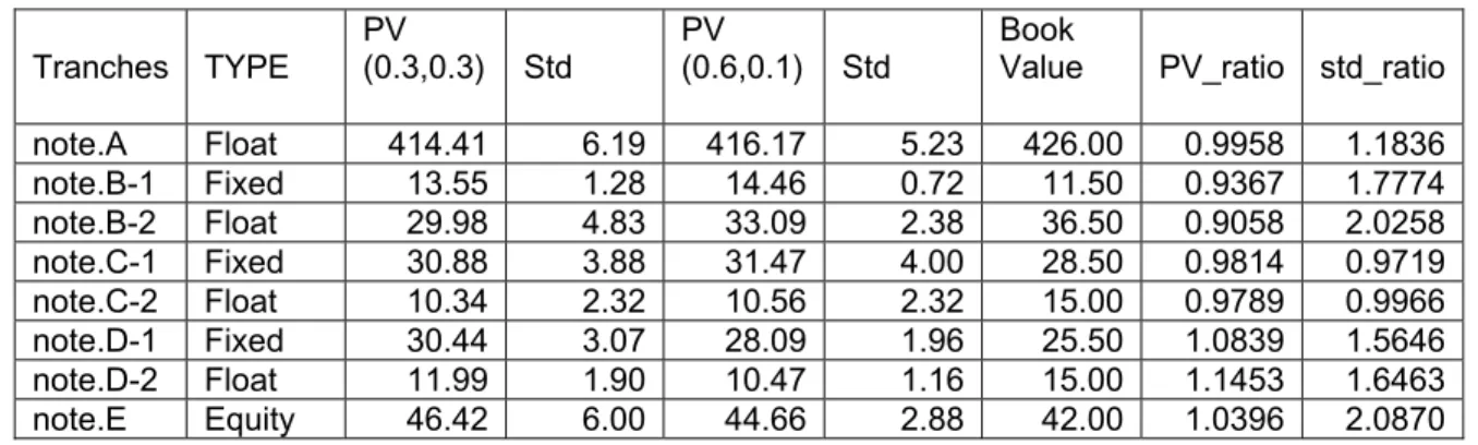
(13) Committee on Banking Supervision (BCBS) document of November 2001, asset correlations were assumed to be a decreasing function of firm probability of default. Lopez (2002) reported the similar results. We set up a CDO with 5 tranches invested on 77 obligors. We assume that there is no reinvestment and liquidation. In the first set, 3 obligors are rated as A, 6 obligors are rated as BBB, 68 obligors are rated as B with constant asset correlation of 0.3. In the second set, 3 obligors are rated as A with correlation 0.6, 6 obligors are rated as BBB with correlation of 0.6, 68 obligors are rated as B with correlation of 0.1. In the third set, 6 obligors are rated as A, 14 obligors are rated as BBB, 57 obligors are rated as B with constant asset correlation of 0.23. In the fourth set, 6 obligors are rated as A with correlation 0.6, 14 obligors are rated as BBB with correlation of 0.6, 57 obligors are rated as B with correlation of 0.1. Thus asset correlations are decreasing as firm probability of default increases with average correlation around 0.23. Table 5 reports the change of market value of the CDO under different default correlations. In both cases, as we switch from constant correlation to decreasing default correlation, the market value of mezzanine increases while the market value of lower tranches decreases.. 13.

(14) References. Collin-Dufresne, P. R. S. Golstein and J. S. Martin, 2000, “The Determinants of Credit Spread Changes,” forthcoming in Journal of Finance. Dai, Q., and K. J. Singleton, 2000, “Specification Analysis of Affine Term Structure Models,” Journal of Finance, 55, 1943-1978. Delianedis, G., and R. Geske, 2001, “The Components of Corporate Credit Spreads,”, Working Paper, UCLA. Duffee, G. R., 1999, “Estimating the Price of Default Risk”, The Review of Financial Studies, 12, no. 1, 197 – 226. Duffie, D., and N. Garleanu, 1999, “Risk and Valuation of Collateralized Debt Obligations,” Working Paper, Stanford University. Duffie, D., and K. J. Singleton, 1997, “An Econometric Model of the Term Structure of Interest-Rate Swap Yields,” Journal of Finance, 52, 1287-1321. Duffie, D., and K. J. Singleton, 1999, “Simulating Correlated Defaults,” Working Paper, Stanford University. Eom, Y. H., J. Helwege, and J. Huang, 2000, Structural Models of Corporate Bond Pricing”, Working Paper, Ohio State University. Elton, E., M. Gruber, D. Agrawal, and C. Mann, 2000, “Explaining the Rate Spread on Corporate Bonds”, forthcoming Journal of Finance. Finger, C., 2002, “A Comparison of Stochastic Default Rate Models,” Working Paper, The RiskMetrics Group. Jarrow, R. A., and S. M. Turnbull, 1995, “Pricing Derivatives on Financial Securities Subject to Credit Risk Spreads,” Journal of Finance, 50, 53-86. Jarrow, R. A., D. Lando and S. M. Turnbull, 1997, “A Markov Model for the Term Structure of Credit Risk Spreads,” The Review of Financial Studies, 10, 481-523. Jones, E. P., S. Mason, and E. Rosenfeld, 1984, “Contingent Claims Analysis of Corporate Capital Structures,” Journal of Finance, 39, 611-625. Lund, J., 1997, “Non-Linear Kalman Filtering Techniques for Term-Structure Models,” Working Paper, Aarhus School of Business. Merton, R. C., 1974, “On the Pricing of Corporate Debt: The Risk Structure of Interest Rates,” Journal of Finance, 29, 449-470. 14.

(15) Skinner, F. S. and A. Diaz, 2000, “On Modeling Credit Risk Using Arbitrage Free Models”, Discussion Paper, ISMA Center, University of Reading.. 15.

(16) Table 1. Estimated Parameters of Treasury and Credit Curves (July 1995 – February 2002) Treasury Coef Std. κ 1r θ 1r σ 1r λ1r κ 2r θ 2r σ 2r λ2 r αr σε RMSE(%). 0.423. 0.064. 0.982. 0.019. 0.017. 0.004. -0.001. 0.200. 0.028. 0.062. 0.144. 0.312. 0.024. 0.003. -0.123. 2.506. -1.058. 0.021. 2.651. 0.130. 1.670. Coef. κh θh σh λh αh σε β1 β2. AAA Std. AA Std. Coef. A Coef. Std. Coef. BBB Std. Coef. BB Std. 0.021. 0.012. 0.014. 0.012. 0.015. 0.012. 0.012. 0.013. 0.026. 0.013. 0.597. 0.042. 0.593. 0.034. 0.595. 0.033. 0.595. 0.028. 0.594. 0.026. 0.008. 0.004. 0.007. 0.003. 0.008. 0.004. 0.008. 0.004. 0.016. 0.007. -0.487. 0.541. -0.489. 0.530. -0.490. 0.508. -0.491. 0.472. -0.491. 0.434. -0.052. 0.271. -0.051. 0.262. -0.050. 0.231. -0.049. 0.198. -0.049. 0.222. 3.684. 0.197. 3.813. 0.206. 3.093. 0.163. 2.329. 0.116. 1.764. 0.067. -0.511. 0.214. -0.510. 0.209. -0.509. 0.181. -0.509. 0.167. -0.508. 0.196. -0.762. 0.167. -0.765. 0.148. -0.765. 0.161. -0.765. 0.194. -0.761. 0.268. 1.420. 1.410. 16. 1.390. 1.440. 1.650.

(17) Table 2. Estimated Parameters of Treasury and Default Curves (July 1995 – February 2002). Treasury Coef Std. κ 1r θ 1r σ 1r λ1r κ 2r θ 2r σ 2r λ2 r αr σε RMSE(%). 0.423. 0.064. 0.982. 0.019. 0.017. 0.004. -0.001. 0.200. 0.028. 0.062. 0.144. 0.312. 0.024. 0.003. -0.123. 2.506. -1.058. 0.021. 2.651. 0.130. 1.670. Coef. κh θh σh λh αh σε β1 β2. AAA Std. AA Std. Coef. A Coef. Std. Coef. BBB Std. Coef. BB Std. 0.043. 0.020. 0.078. 0.016. 0.056. 0.007. 0.064. 0.013. 0.017. 0.066. 0.641. 0.143. 0.602. 0.041. 0.711. 0.045. 0.626. 0.054. 0.591. 15.308. 0.006. 0.002. 0.032. 0.009. 0.030. 0.006. 0.031. 0.007. 0.001. 0.008. -0.413. 0.521. -0.373. 0.388. -0.076. 0.116. -0.284. 0.285. -0.487. 16.352. -0.063. 0.259. -0.069. 0.269. -0.083. 0.225. -0.082. 0.248. -0.053. 15.706. 4.277. 0.243. 1.187. 0.059. 1.100. 0.060. 1.156. 0.059. 10.451. 1.732. -0.522. 0.169. -0.526. 0.240. -0.541. 0.215. -0.539. 0.235. -0.513. 0.849. -0.719. 0.150. -0.771. 0.132. -0.753. 0.147. -0.668. 0.158. -0.755. 0.357. 1.360. 3.720. 17. 1.830. 3.300. 11.990.

(18)

(19) Table 3. Fitted Credit and Default Spreads (July 1995 – February 2002) Credit spread Median Std AAA AA A BBB BB. 62.50 66.00 87.00 118.50 238.00. Default spread Median Std. 27.38 31.76 38.23 49.84 87.01. 4.04 5.79 12.39 22.65 81.31. Ratio. 3.66 4.98 9.76 16.64 28.27. 6.47% 8.77% 14.24% 19.11% 34.16%. Table 4. Credit and Default Spread Correlations (July 1995 – February 2002) Credit Spread Correlations AAA AAA AA A BBB BB. AA. 1.00 0.98 0.93 0.91 0.84. A 0.98 1.00 0.95 0.93 0.89. BBB 0.93 0.95 1.00 0.95 0.94. BB 0.91 0.93 0.95 1.00 0.95. 0.84 0.89 0.94 0.95 1.00. Default Spread Correlations AAA AAA AA A BBB BB. 1.00 0.89 0.85 0.77 0.47. AA. A 0.89 1.00 0.84 0.72 0.43. 19. BBB 0.85 0.84 1.00 0.84 0.65. BB 0.77 0.72 0.84 1.00 0.84. 0.47 0.43 0.65 0.84 1.00.

(20) Table 5. Impact of default correlation on cash-flow CDO’s market values. A (3), BBB (6), B & B- (68) Tranches. TYPE. PV (0.3,0.3). note.A note.B-1 note.B-2 note.C-1 note.C-2 note.D-1 note.D-2 note.E. Float Fixed Float Fixed Float Fixed Float Equity. 414.41 13.55 29.98 30.88 10.34 30.44 11.99 46.42. PV (0.6,0.1). Std 6.19 1.28 4.83 3.88 2.32 3.07 1.90 6.00. 416.17 14.46 33.09 31.47 10.56 28.09 10.47 44.66. Book Value. Std 5.23 0.72 2.38 4.00 2.32 1.96 1.16 2.88. 426.00 11.50 36.50 28.50 15.00 25.50 15.00 42.00. PV_ratio. std_ratio. 0.9958 0.9367 0.9058 0.9814 0.9789 1.0839 1.1453 1.0396. 1.1836 1.7774 2.0258 0.9719 0.9966 1.5646 1.6463 2.0870. PV_ratio. std_ratio. 0.9996 0.9850 0.9771 0.9726 0.9608 1.0405 1.0672 1.0311. 0.8744 25.5706 5.8705 1.4396 1.3889 1.4682 1.4245 2.4106. A (6), BBB (14), B & B- (57) Tranches. TYPE. PV (0.23,0.23). note.A note.B-1 note.B-2 note.C-1 note.C-2 note.D-1 note.D-2 note.E. Float Fixed Float Fixed Float Fixed Float Equity. 416.54 14.69 34.26 34.29 12.29 31.65 12.69 40.64. Std 1.51 0.47 3.55 6.97 4.61 6.18 4.21 8.77. PV (0.6,0.1) 416.71 14.91 35.07 35.26 12.79 30.42 11.89 39.41. 20. Std 1.73 0.02 0.61 4.84 3.32 4.21 2.95 3.64. Book Value 426.00 11.50 36.50 28.50 15.00 25.50 15.00 42.00.

(21) Figure 1. Term Structure of Median Fitted Credit Spreads July 1995 – February 2002. 350 300 AAA. 250. AA. 200. A. 150. BBB. 100. BB. 50 0 0.60. 1.00. 3. 5. 7. 21. 10.00 20.00 30.00.

(22) 22 Jan-02. Jul-01. Jan-01. Jul-00. Jan-00. Jul-99. Jan-99. Jul-98. Jan-98. Jul-97. Jan-97. Jul-96. Jan-96. Jul-95. Jan-02. Jul-01. Jan-01. Jul-00. Jan-00. Jul-99. Jan-99. Jul-98. Jan-98. Jul-97. Jan-97. Jul-96. Jan-96. Jul-95. Figure 2. Fitted Credit and Default Spreads (July 1995 – February 2002). 600. 500. 400 AA. AAA. 300 A. 200 BBB. BB. 100. 0. 140. 120. 100. AAA. 80. AA. 60. A. BBB. 40. BB. 20. 0.

(23)

No results found