NEURAL NETWORKS
Master’s thesisExaminer: Professor Karen Eguiazarian (Egiazarian)
The examiner and topic of the thesis were approved on 31 October 2018
ABSTRACT
ANSSE SAARIMÄKI: Single Image Super-Resolution Using Convolutional Neural Networks
Tampere University of Technology
Master of Science Thesis, 57 pages, 3 Appendix pages December 2018
Master’s Degree Programme in Information Technology Major: Audio-Visual Signal Processing
Examiner: Professor Karen Eguiazarian (Egiazarian)
Keywords: Single image super-resolution, convolutional neural networks, image enhancement
Enlargement of images is a common need in many applications. Although increasing the pixel count of an image is easy with simple interpolation methods, those fail to increase the amount of details in the image. Single image super-resolution (SISR) aims to solve this ill-posed problem of producing a high resolution (HR) image from a given low resolution (LR) image. A single LR image has always an infinite number of corresponding LR images, but some of those are more probable than others. This probability density can be estimated with machine learning techniques, and the most probable HR image can be constructed based on that estimate.
In recent years artificial neural networks have become the most popular machine learning methods. Convolutional neural networks (CNN) are a subtype of them, inspired by the human visual system. They are used extensively in all fields of image processing, including single image super-resolution. In this thesis different CNN based methods for SISR are compared, and their performance is analyzed using both quantitative and qualitative methods. In total four CNN methods were chosen, and they were compared to three other methods. One of the reference methods was based on more traditional machine learning, and the two others were based on self-similarity of the input images. In contrast to machine learning approach, self-similarity based methods utilize only information in the input image and do not require any training on external images.
The results show that CNN based methods outperform the alternative approaches in both quantitative metrics and qualitative analysis. The methods perform especially well with images that have clear structures and sharp edges, but highly textured images tend to be problematic. Six of the methods aim to minimize pixel-wise reconstruction error, which leads to overly smooth output on textured areas. One method was instead designed to maximize the perceptual quality of the images, at the cost of increased reconstruction error. It was able to generate very realistic textures in some cases, but had a tendency to hallucinate very implausible textures into flat areas. Also other CNN based methods tended to create erroneous but plausible details, which might be misleading in critical applications like medical imaging. CNN based SISR is more suitable for entertainment and other consumer applications, especially when the perceptually optimized methods are developed further.
TIIVISTELMÄ
ANSSE SAARIMÄKI: Yhden kuvan superresoluutio konvoluutioneuroverkkoja käyt-täen
Tampereen teknillinen yliopisto Diplomityö, 57 sivua, 3 liitesivua Joulukuu 2018
Tietotekniikan diplomi-insinöörin tutkinto-ohjelma Pääaine: Audio-Visual Signal Processing
Tarkastaja: professori Karen Eguiazarian (Egiazarian)
Avainsanat: Yhden kuvan superresoluutio, konvoluutioneuroverkot, kuvanparannus
Digitaalisten kuvien suurentaminen on tarpeellista monissa sovellutuksissa, ja se on helppoa suorittaa yksinkertaisilla interpolaatimenetelmillä. Ne eivät kuitenkaan kykene lisäämään kuvan yksityiskohtia, ja varsinainen resoluutio jää samaksi kasvaneesta pikselimäärästä huolimatta. Korkeamman resoluution kuvan tuottaminen yhdestä matalan resoluution kuvasta on inversio-ongelma, jonka yhden kuvan super-resoluutio pyrkii ratkaisemaan. Yhdellä matalan resoluution kuvalla on aina ääretön määrä korkean resoluution vastineita, mutta osa niistä on aina todennäköisempiä kuin toiset. Tätä todennäköisyysjakaumaa voi estimoida koneoppimismenetelmien avulla, ja todennäköisin korkean resoluution kuva voidaan muodostaa tämän estimaatin pohjalta.
Viime vuosina keinotekoiset neuroverkot ovat muodostuneet suosituimmaksi lähestymista-vaksi koneoppimiseen. Konvoluutioneuroverkot kuuluvat tähän ryhmän, ja ne ovat saaneet inspiraationsa ihmisen näköhermostosta. Niiden käyttö on erittäin yleistä kaikilla kuvan-käsittelyn aloilla, mukaan lukien yhden kuvan superresoluutiossa. Tässä diplomityössä vertaillaan erilaisia konvoluutioverkkoihin perustuvia superresoluutiomenetelmiä, ja niiden suorituskykyä analysoidaan sekä kvantitatiivisesti että kvalitatiivisesti. Neljää valittua konvoluutioverkkopohjaista menetelmää verrataan kolmeen muuhun, joista yksi perus-tuu perinteisempään koneoppimiseen. Kaksi muuta menetelmää hyödyntävät tyypillisissä kuvissa toistuvia samankaltaisia elementtejä, eivätkä ne tarvitse opettamista ulkoisella kuvadatalla kuten koneoppimismenetelmät.
Tulokset osoittavat, että konvoluutioverkkopohjaiset menetelmät suoriutuvat vaihtoehtoisia menetelmiä paremmin sekä kvantitaviisessa että kvalitatiivisessa analyysissa. Menetelmät suoriutuvat erityisen hyvin kuvista joissa on selkeitä rakenteita ja teräviä rajoja, mutta voi-maakkaasti teksturoidut kuvat tuottavat ongelmia. Menetelmistä kaikki paitsi yksi pyrkivät minimoimaan pikselikohtaisesti lasketun rekonstruointivirheen, joka johtaa liian tasai-siin pintoihin tekstuuripitoisilla alueilla. Yksi menetelmistä pyrkii maksimoimaan kuvien havainnoidun laadun rekonstruointivirheen kustannuksella, ja se kykeneekin tuottamaan realistisen näköisiä tekstuureja sen ansiosta. Useimmissa tapauksissa sillä oli kuitenkin taipumuksena tuottaa tekstuureja alueille joissa niitä ei kuuluisi olla, ja lopputulos oli erittäin epäuskottava. Myös muilla konvoluutioverkkoja käyttävillä menetelmillä oli tai-pumusta generoida virheellisiä, mutta uskottavan näköisiä yksityiskohtia. Tämä rajoittaa niiden soveltuvuutta kriittisiin käyttökohteisiin, kuten lääketieteelliseen kuvantamiseen. Konvoluutioverkkopohjainen yhden kuvan superresoluutio soveltuukin paremmin viih-desovelluksiin ja muuhun kuluttajakäyttöön, erityisesti mikäli havainnoidulle laadulle optimoidut menetelmät kehittyvät pidemmälle.
PREFACE
This thesis was started while I was working as a research assistant in the Computational Imaging Group of the Signal Processing Laboratory at Tampere University of Technology. Most of the background research for this thesis was done during that employment, but the thesis is otherwise independent from the project I was working on.
First of all I want to thank my supervisor and examiner, professor Karen Eguiazarian, for his guidance during all phases of this project, and for the opportunity work in his research group. Also I want thank my former colleague Cristóvão Cruz, who helped me numerous times, and created the MATLAB testbench used for testing the methods in this thesis. Last but not least, I want to thank my wife Nyyti, for her support and patience during this prolonged project.
In Tampere, Finland, on 20 November 2018
CONTENTS
1. INTRODUCTION ... 1
2. THEORETICAL BACKGROUND... 3
2.1 Sampling and interpolation ... 3
2.2 Image quality metrics... 11
2.3 Machine learning basics... 13
2.3.1 Types of ML tasks... 14
2.3.2 Supervised and unsupervised learning ... 15
2.3.3 Datasets and model performance... 16
2.4 Feedforward neural networks... 17
2.4.1 Activation layers ... 18 2.4.2 Loss functions... 19 2.4.3 Optimization ... 20 2.4.4 Convolutional layers ... 23 3. SUPER-RESOLUTION... 27 3.1 Multi-image super-resolution... 28
3.2 Single image super-resolution... 29
3.3 Self-similarity based SISR... 29
3.4 Traditional Machine Learning Methods for SISR... 30
3.5 Convolutional Neural Networks based SISR ... 31
3.5.1 HR Networks for SISR ... 32
3.5.2 LR Networks for SISR ... 34
3.5.3 Networks Optimized for Perceptual Quality... 37
4. TESTING METHODOLOGY ... 38
5. RESULTS ... 40
6. CONCLUSIONS... 49
REFERENCES ... 52
LIST OF FIGURES
Figure 2.1. Illustration of a continuous signal and its sampling process.... 4
Figure 2.2. Impulse responses of NN, linear, cubic and sinc interpolation filters.... 7
Figure 2.3. Amplitude responses of NN, linear, cubic and sinc interpolation filters. 8 Figure 2.4. Example images produced by upsampling with different interpolation methods.... 10
Figure 2.5. A simple multilayer perceptron.... 18
Figure 2.6. One-dimensional convolution with and without input padding.... 24
Figure 2.7. Examples of one-dimensional strided convolution and deconvolution.. 24
Figure 2.8. Two-dimensional deconvolution with stride 12 [51].... 25
Figure 2.9. Two-dimensional sub-pixel convolution with scaling factor of 2 [51]... 26
Figure 3.1. The network structure of SRCNN [6].... 33
Figure 3.2. The network structure of VDSR [30].... 33
Figure 3.3. The network structure of ESPCN for scale factor ofr [50].... 34
Figure 3.4. The network structure of SRResNet [35].... 35
Figure 3.5. The network structures of EDSR and MDSR [30].... 35
Figure 3.6. The network structure of D-DBPN [21].... 36
Figure 3.7. The network structure of ProSR [61].... 36
Figure 5.1. Patches extracted from image 66 from Urban100 dataset super-resolved with scaling factor of 4.... 43
Figure 5.2. Patches extracted from image 92 from Urban100 dataset super-resolved with scaling factor of 4.... 44
Figure 5.3. Patches extracted from image 858 from DIV2K validation dataset super-resolved with scaling factor of 4.... 45
Figure 5.4. Image 238 from TAMPERE17 dataset super-resolved with scaling factor of 4.... 46
Figure 5.5. Image 256 from TAMPERE17 dataset super-resolved with scaling factor of 4.... 47
Figure A.1. Image 66 from Urban100 dataset super-resolved with scaling factor of 4.... 58
Figure A.2. Image 92 from Urban100 dataset super-resolved with scaling factor of 4.... 59
LIST OF TABLES
Table 4.1. Summary of the compared SR methods.... 38
Table 5.1. Average PSNR and SSIM scores for scaling factor of 2.... 40
Table 5.2. Average PSNR and SSIM scores for scaling factor of 3.... 41
Table 5.3. Average PSNR and SSIM scores for scaling factor of 4.... 41
Table 5.4. Average processing time of a single image for each method, dataset and scaling factor.... 42
LIST OF ABBREVIATIONS
CPU central processing unit
GPU graphics processing unit
HR high resolution
LR low resolution
MISR multi-image super-resolution
ML machine learning
MSE mean square error
NN nearest neighbor
PSNR peak-signal-to-noise ratio SGD stochastic gradient descent SISR single image super-resolution
SR super-resolution
1. INTRODUCTION
Digital images have become ubiquitous in our everyday lives, ranging from consumer applications like computer generated graphics on a website and holiday photos taken with a cellphone camera, to critical professional applications like medical imaging and surveillance camera footage. As images have become more common, their quality has increased. There are multiple aspects of image quality, but one of the most important ones is the resolution of an image. Resolution has multiple definitions in the context of imaging, and even more outside it, but we will be discussing only spatial resolution of the images. It can be defined as the number discrete points in an image that can be distinguished from each other [48, p. 18].
The resolution of digital images is usually expressed as number of pixels in the image, although it might not correspond with the actual resolution as defined above. Number of pixels sets the upper limit for resolution, but it might be lower depending on the image formation process. This is a common issue with typical digital cameras, where the number of pixels is dictated by the sensor, but resolution is lower due to demosaicking, low quality optics, focusing issues, denoising etc.
Similar problem occurs when we want to increase the size of a digital image, for example to view it on a higher resolution display. Number of pixels in the image must correspond to the display resolution and the desired image size. It can be achieved by interpolating the image, but the actual resolution is not increased while the number pixels increases. This leads to blurry looking images, as the amount of details in the image does not increase. This limit is present in all digital imaging systems, and it cannot be surpassed by any interpolation method.
Super-resolution (SR) tries to overcome this limit and produce a higher resolution image, which actually contains details not visible in the source image. There are two distinct ways to achieve this. The first, and more traditional one is the multi-image super-resolution (MISR) approach, which produces a high resolution (HR) image from multiple low resolution (LR) images depicting the same scene. Each of the input images should contain unique information for MISR to work, meaning that the images should have sub-pixel level displacements between them. This way the pixels are sampled from unique locations, and the effective total resolution is higher than the resolution of any single input image. MISR has a very limited applicability, as often only a single LR image is available. This has lead to development of single image super-resolution (SISR) methods. There is always an infinite number of unique HR images that could correspond to a single LR image, and SISR methods can only make an assumption of what the HR image could look like. MISR
methods on the contrary can extract actual HR details hidden in the LR images.
SISR can be performed by utilizing a large image database with both LR images and their corresponding HR images. Machine learning techniques can be then used to learn the most probable, input content dependable mapping from LR to HR image [54, 6, 30, 36]. Another way is to utilize the self-similarity of the input image [9, 13, 26, 4]. Especially natural images tend to have elements that repeat throughout the image, possibly with different scale, rotation, and other types of affine transformations. When processing the image patch-by-patch, the similar patches can be treated like individual images and processed with MISR methods.
Convolutional neural networks (CNN) are the most popular machine learning approach used in state-of-the-art SISR research [53, 56]. They are a specific subtype of artificial neural networks, that are machine learning methods originally inspired by the workings of biological brains [19, p. 13]. CNNs are a relatively old concept [34], but their popularity surged to its current state only after 2012, when Krizhevsky et al. [33] published their AlexNet image classification network. It outperformed all of the previous methods by a clear margin, and changed the field of machine learning research completely [19, p. 24]. CNNs were first applied to SISR in 2014 by Dong et al. [6], and since it has become the most prominent approach in state-of-the-art SISR research [3, 53, 56]. In this thesis we will give an overview of CNN based super-resolution in a form of a literature review, and discuss both the state-of-the-art methods and their historical background. Additionally, a comparison of selected methods is performed, with both quantitative and qualitative analysis of their performance. A total of seven methods were chosen to represent distinct SISR approaches, with four of them being based on CNNs, two on self-similarity, and one on classical machine learning. The results show that CNN based methods have unparalleled performance in terms of image quality, and SISR research has made huge leaps through the usage of CNNs.
For understanding the CNN based SISR methods, their theoretical foundations are discussed in Chapter 2. To explain the problem SR is trying to solve, general theory on digital sampling and interpolation is outlined first. After that we discuss the image quality metrics used for quantitative comparison of the SISR methods. Last part of that chapter will explain the theory behind CNNs, starting with basics of machine learning and ending with CNN specific details.
Chapter 3 discusses the different SR methods, including MISR, self-similarity SISR, and machine learning based SISR. The main focus will be on CNN based methods, and they are explained in more depth than alternative approaches. The seven chosen methods are also analyzed in that chapter. Chapter 4 describes the testing setup used in the comparison, and the results are shown and analyzed in Chapter 5. Findings are summarized in Chapter 6, which also discusses the potential applications and topics for further research.
2. THEORETICAL BACKGROUND
As a basis for the super-resolution problem in general, a brief analysis of sampling and interpolation theory is given in Section 2.1. Section 2.2 will give an overview of image quality metrics used for performance comparison of SR algorithms in this thesis. Section 2.3 explains the main concepts of general machine learning and serves as a primer for the next section. Section 2.4 explains the class of artificial neural networks known as feed-forward networks, of which convolutional networks are a part of. That section will also explain the basics of convolutional networks, but the next chapter demonstrates how to apply them to super-resolution.
2.1
Sampling and interpolation
To really understand the problem super-resolution is trying to solve, one has to understand the limitations imposed by the discrete sampling process and why pure interpolation cannot overcome them. Digital imaging is essentially about sampling a two-dimensional continuous signal, e.g. the scene "seen" by the optics of a camera. The same principles apply to two-dimensional sampling as to the one-dimensional cases like digital audio. Naturally the human visual system works very differently in comparison to the auditory system, and thus many of the methods applied for audio processing are not usable in imaging context even when they work theoretically. Basics are nevertheless the same, and thus we will be mostly discussing the one-dimensional case in this section.
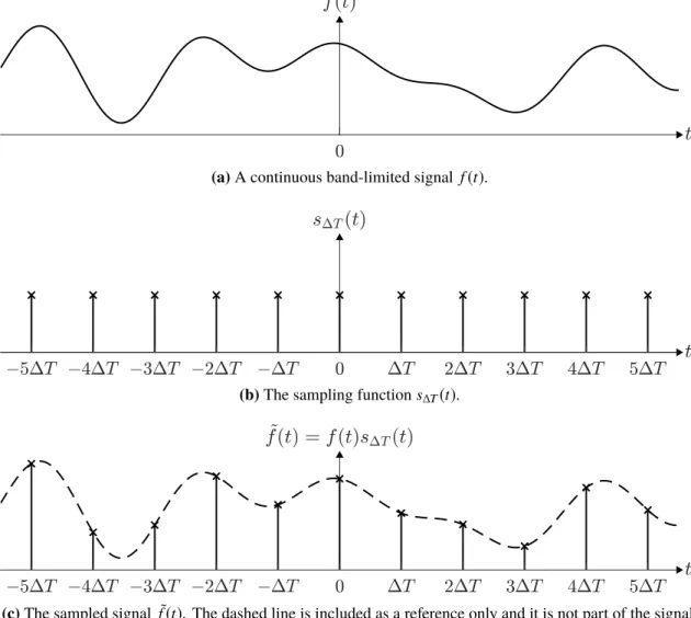
Let us consider a continuous band-limited real-valued function f(t),t∈R. A uniformly sampled version of it is ˜ f(t)= f(t)s∆T(t)= ∞ ∑ n=−∞ f(t)δ(t−n∆T),n∈N, (2.1)
where∆T is the sampling interval,δ(x)is the unit discrete impulse
δ(x)= { 1 x=0 0 x,0, (2.2) and s∆T(t)= ∞ ∑ n=−∞ δ(t−n∆T) (2.3)
is the sampling function equal to a train of unit impulses with∆T intervals. An example of function f(t), its sampled version ˜f(t), and the sampling function s∆T(t)are illustrated
(a)A continuous band-limited signal f(t).
(b)The sampling functions∆T(t).
(c)The sampled signal ˜f(t). The dashed line is included as a reference only and it is not part of the signal.
(d)The discrete sample sequence fk.
Figure 2.1. Illustration of a continuous signal and its sampling process.
in Figure 2.1. We can also denote the sampled function as a sequence of discrete values
fk = f(tk),k ∈N, in whichtk=k∆T is the sample location. [18, p. 212] The Fourier transform of function f(t)is
F{f(t)}=F(ω)=
∫ ∞ −∞
f(t)e−j2πωt dt, (2.4)
whereω is the frequency. Since the function f(t)is band-limited, there exists a frequency
component of the function f(t). The Fourier transform of the sampling functions∆T(t)is F{s∆T(t)}=S∆T(ω)= 1 ∆T ∞ ∑ n=−∞ δ(ω− n ∆T ) , (2.5)
which is also an impulse train, but with an interval of ∆1T. The Fourier transform of the sampled function ˜f(t)is thus ˜F(ω)=F{f˜(t)}=F{f(t)s∆T(t)}. As a Fourier transform of a product of two functions is the convolution of Fourier transforms of those functions, the sampled function in Fourier-domain is
˜ F(ω)=F{f(t)s∆T(t)} =F(ω) ∗S∆T(ω) = 1 ∆T ∞ ∑ n=−∞ F ( ω− n ∆T ) , (2.6)
where the∗is the convolution operation. [18, p. 212–213]
The Nyquist-Shannon sampling theorem states that f(t)can be perfectly reconstructed from ˜f(t)when the sampling rate ∆1T is greater than twice the highest frequency component
ωmax of the function f(t). The frequency limit of 2∆1T is called the Nyquist rate (or the Nyquist frequency), and it is the highest frequency that can be recovered from the sampled signal. The case ofωmax< 2∆1T is called oversampling,ωmax= 2∆1T is critical sampling and
ωmax> 2∆1T is undersampling. In the case of oversampling, the original function f(t)can be perfectly recovered from the sampled version ˜f(t)by filtering out all the frequencies greater thanωmaxwith ideal low-pass filter. In the case of undersampling, the frequencies of F(ω)higher than 2∆1T will be overlapping with the frequencies below. This effect is called aliasing, and it prevents a perfect reconstruction and causes noticeable artifacts in the sampled signal. [18, p. 214–215]
The perfect reconstruction using an ideal low-pass filter can be expressed mathematically in the Frequency domain as
F(ω)=H(ω)F(ω),˜ (2.7) where H(ω)= { ∆T −ωc≤ω ≤ωc 0 otherwise (2.8)
is the filter’s frequency response andωc= 2∆1T > ωmaxis the filter’s cutoff frequency. The original signal f(t)can then be acquired fromF(ω)using inverse Fourier transform:
f(t)=F−1{F(ω)}=
∫ ∞ −∞
F(ω)ej2πωt dω (2.9)
This filtering can also presented in spatial domain using convolution as
where
h(t)=F−1{H(ω)}=2ωc∆Tsinc(2ωc∆T t)=sinc(t)=
sin(πt)
πt (2.11)
is the filter’s impulse response. This ideal filter will attenuate all of the frequencies over
ωc, leaving only the original signal f(t). [18, p. 215–216, 220]
In practice this perfect sampling can never be achieved. First problem arises with the notion of a continuous band-limited signal, as no signal of finite length can be truly band-limited [18, p. 218]. All practical images are finite in length, thus there will always be some aliasing introduced in the sampling process. The aliasing cannot be completely removed, although it can be attenuated greatly with proper pre-filtering. Second problem is the ideal low-pass filter required for the perfect reconstruction, as its impulse response, the sinc-function, has infinite length.
Although the perfect reconstruction of f(t)is practically impossible, an adequate approx-imation ˆf(t) ∼ f(t)could be achieved through convolution ˆf(t)=hˆ(t) ∗ f˜(t)with some other interpolation filter ˆh(t). For ˆh(t)to be an interpolation filter, it has to satisfy the following requirements: ˆ h(t)= { 1 t=0 0 t=n∆T,|n|=1,2,... (2.12)
This guarantees that the function values at sample locations will remain unchanged, thus
ˆ
f(n∆T)= f˜(n∆T)= f(n∆T),∀n∈N. For simplicity we will assume from now on that the sampling interval∆T =1, so that that the samples are always located attk =k,k ∈N. In the context of this thesis the actual sampling interval is irrelevant and it is also unknown for all the images used. Thus the interpolation can be represented in discrete terms as
ˆ f(t)= ∞ ∑ k=−∞ fkhˆ(t−k), (2.13)
where fk = f(k)is the sequence of sampled values. [29]
The simplest possible way to interpolate is to use the so-called nearest neighbor (NN) method, which chooses the value of the nearest sample as the interpolated value [18, p. 65]. In terms of filter impulse response, the method is defined as
hnn(t)= {
1 −0.5<t ≤0.5
0 otherwise. (2.14)
Although it is mathematically very simple and computationally efficient, NN often produces visually unpleasing results. Images upsampled with NN interpolation typically contain blocky artifacts, which can be seen in Figure 2.4(a). Although those artifacts are intuitively explained with the filter’s impulse response, their source is also easily visible in the filter’s frequency response
Hnn(ω)=F{hnn(t)}=sinc(ω)=
sin(πω)
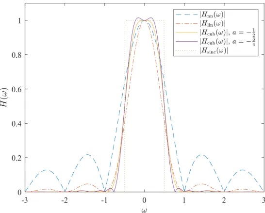
The amplitude response|Hnn(ω)|is illustrated in Figure 2.3, which clearly shows the poor performance when compared to the ideal reconstruction filter |Hsinc(ω)|. Frequencies above the Nyquist-rate are attenuated inadequately and the resulting reconstruction is far from ideal. -3 -2 -1 0 1 2 3 -0.2 0 0.2 0.4 0.6 0.8 1
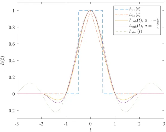
Figure 2.2. Impulse responses of NN, linear, cubic and sinc interpolation filters.
A simple improvement over NN interpolation is to use the two nearest neighbors, and linearly interpolate between them [18, p. 65]. In two-dimensional cases the method is commonly called bilinear interpolation, and four nearest neighbors are used. The impulse response of the one-dimensional filter is defined as
hlin(t)= {
1− |t| |t|<1
0 otherwise,
(2.16)
and its frequency response is
Hlin(ω)=F{hlin(t)}=sinc2(t)=
sin2(πω)
π2ω2 . (2.17)
With this filter the resulting image is notably smoother, but there is still visible jaggedness around the sharpest edges, as can be seen in Figure 2.4(b). Also the amplitude response (Fig. 2.3) has still room for improvement.
A commonly used compromise between computational complexity and output image quality is the cubic convolution interpolation introduced by Keys in 1981 [29]. We are
-3 -2 -1 0 1 2 3 0 0.2 0.4 0.6 0.8 1
Figure 2.3. Amplitude responses of NN, linear, cubic and sinc interpolation filters.
referring its two-dimensional case as bicubic interpolation, although usage of that word is ambiguous in other literature. The one-dimensional cubic method interpolates based on the four nearest samples using a kernel defined as
hcub(t)= ⎧ ⎪ ⎪ ⎪ ⎪ ⎨ ⎪ ⎪ ⎪ ⎪ ⎩ (a+2)|t|3− (a+3)|t|2+1 0<|t| ≤1
a|t|3−5a|t|2+8a|t| −4a 1<|t| ≤2
0 otherwise,
(2.18)
whereais an constant affecting the properties of the kernel. Keys proved that by setting the parameter asa=−1
2, the interpolated signal ˆf(t)will converge fastest towards the original
signal f(t), when the sampling interval approaches zero [29]. Using this value the kernel reduces to hcub(t)= ⎧ ⎪ ⎪ ⎪ ⎪ ⎨ ⎪ ⎪ ⎪ ⎪ ⎩ 3 2|t| 3−5 2|t| 2+1 0< |t| ≤1 −1 2|t| 3+5 2|t| 2−4|t|+2 1< |t| ≤2 0 otherwise. (2.19)
and its frequency response becomes
Hcub(ω)=F{hcub(t)}=
sin3(πω)(−2πωcos(πω)+3 sin(πω))
This form is used e.g. in MATLAB’simresize function [39], which is the reference resampling method in this thesis. Other values ofaare also possible, and e.g. OpenCV uses a =−3
4 instead [42]. Impulse and amplitude responses for both values of a are
demonstrated in Figures 2.2 and 2.3 respectively. For both options the impulse response is a quite close approximation of the sinc filter for|t|<1, and they include a negative lobe in 1< |t|<2 like the sinc filter. The amplitude shows a lot higher attenuation for the stop-band
frequencies than the previous two methods and the attenuation is less pronounced for the higher pass-band frequencies.
Resulting images with bicubic upsampling are presented in Figures 2.4(c) and 2.4(d) with
a=−1
2 anda=− 3
4respectively. The results for both are very similar, with sharper edges
and less jaggedness in comparison to bilinear upsampling. Due to the negative lobes of the filter kernels, there is a notable ringing visible in high contrast edges such as in the back of the man. It is more pronounced in the image produced witha=−3
4. Although this ringing
is mostly an unwanted effect it does increase the perceived sharpness and thus helps in some cases.
An approximation of the ideal reconstruction with a sinc filter has been included for comparison in Figure 2.4(e). As was said earlier, the truly ideal reconstruction cannot be achieved with finite length signal, which has been circumvented in this example by padding the input image with infinite zeros. Effectively this truncates the filter kernel to the size of the input image and makes the computation tractable. This zero-padding will lead to large amounts of ringing around the image borders and makes the image unusable, but it does highlight the fundamental problem of this ideal reconstruction method. Every sharp brightness transition in the input image will lead to similar ringing artifacts, which will be repeated around the edges until attenuated below the quantization noise level. Thus the ideal reconstruction would be a poor choice for image interpolation, even if it were attainable in practice.
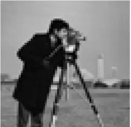
The upsampled images in Figures 2.4(a)–2.4(e) have all been produced by first downsampling the original image (Fig. 2.4(f)) by a factor of 4 and then upsampled using the corresponding interpolation methods and scaling factor of 4. The downsampling method is using the bicubic filter and it is described in more detail below. This is the scheme that will be utilized in this thesis also for comparing the super-resolution methods. Included in the figures are PSNR (peak-signal-to-noise ratio) scores for the upsampled images, for which higher value means higher similarity with the ground truth image (the original high resolution image). The PSNR score and other image quality metrics will be discussed in the Section 2.2. To resize the images in general, we can just utilize the equation 2.13 and set the new sample locations as t = n∆sT, where s is the image scaling factor. This works well for upsampling(s>1), but with downsampling (s<1) there is a huge risk of aliasing. This
can be alleviated by using an anti-aliasing (AA) filter, which attenuates the frequencies above the new Nyquist-rate from the interpolated image. AA-filter is essentially a low-pass filter just like the interpolation filter, but with a lower cut-off frequency. Thus we can
(a)Nearest neighbour (PSNR: 21.65 dB) (b)Bilinear (PSNR: 22.25 dB)
(c)Bicubic,a=−1
2 (PSNR: 22.68 dB) (d)Bicubic,a=− 3
4 (PSNR: 22.78 dB)
(e)Sinc (PSNR: 22.08 dB) (f)Ground truth
Figure 2.4. Example images produced by upsampling with different interpolation methods. The ground truth image (f) has been first downsampled with scaling factor of1/4to produce a low resolution input. Images a–e have been upsampled from that LR image with
achieve the goal with a single filter, by lowering the cut-off frequency of the interpolation filter. The cut-off frequency is inversely proportional to the width of the filter kernel [60, p. 374]. Thus with an image scaling factor of s<1 and an interpolation filter ˆh(t), the desired anti-aliasing filterhaa(t)will become
haa(t)=sh(stˆ ). (2.21)
The resulting interpolation kernel will have a support 1s wider than the original un-dilated kernel. This way of producing a downsampling kernel is appropriate for all interpolation methods other than the nearest-neighbour, which should select the single nearest neighbour also for all the pixels of a downsampled image. This scheme is used also in MATLAB [38], and it will also be used when producing the low-resolution input images for testing the SR methods.
2.2
Image quality metrics
Image enhancement methods like super-resolution are typically used to produce images for humans to view, and thus maximizing the perceived quality of the output images is important. The only way to get a reliable estimate of the perceived quality, is to test with a large group of people, and a large dataset of different images. The images should have different types and levels of degradations, and they should be processed with multiple competing methods. The relative performance of the methods would then be compared using the mean opinion score (MOS) collected from those images [45]. This is obviously a very laborious task, and practically impossible to conceive during the development phase of a method. Thus there is a need for some quantitative image quality metric that can be easily calculated for any image. Numerous image quality metrics have been developed for this task, and they can be coarsely divided into two subgroups: signal fidelity metrics and perceptual visual quality metrics [37].
Signal fidelity metrics are the traditional methods like mean absolute error, mean square error (MSE), signal-to-noise ratio (SNR), peak-signal-to-noise ratio (PSNR), and their close relatives [37]. These are simple to calculate and well justified by the underlying physics, but they are not designed specifically for measuring image quality. They are widely known to correlate poorly with the perceived quality, but they are nevertheless universally used in different image processing tasks [12, 37, 45].
PSNR is the de-facto metric used in modern super-resolution research [6, 11, 26, 30, 35, 36, 41, 53, 55, 56], thus it chosen also for this thesis. PSNR is based on MSE, which is defined as MSE(G,D)= 1 nm n−1 ∑ i=0 m−1 ∑ j=0 ( Gi,j−Di,j)2, (2.22)
whereGis the reference (i.e. ground truth) image andDis the degraded image [24]. Both are grayscale images represented by matrices of sizen×m. PSNR itself is defined as
PSNR(G,D)=10 log10 ( MaxG2 MSE(G,D) ) , (2.23)
where MaxG is the highest possible brightness value forG(andD) [1]. For 8 bit grayscale images the value is MaxG =255.
PSNR is considered to be a poor estimator of perceived image quality, which motivates the use of perceptual visual quality metrics. Structural similarity index measure (SSIM) by Wang et al.[62] is one such metric and a very common choice to accompany PSNR in super-resolution research [11, 26, 30, 35, 36, 41, 53, 56]. SSIM is calculated locally for each pixel of the imagesG, andDwith the equation
SSIM(g,d)=l(g,d)c(g,d)s(g,d), (2.24)
where vectorsg={gi|i=0,1,· · ·,k−1}andd={di|i=0,1,· · ·,k−1}represent thek-pixel local neighborhoods of corresponding pixels from images G and D. The term l(g,d)
corresponds to luminance,c(g,d)to contrast ands(g,d)to structural similarity of the pixel neighborhoods, and they are defined as
l(g,d)= 2µgµd+c1 µ2 g+µ2d+c1 (2.25) c(g,d)= 2σgσd+c2 σ2 g+σd2+c2 (2.26) s(g,d)= σgd+c3 σgσd+c3 . (2.27)
The local statisticsµg, µd,σg,σd andσgdare estimated from 11×11 pixel neighborhood weighted with a circular-symmetric Gaussian windoww={wi|i=0,1,· · ·,k−1}, which has standard deviation of 1.5 samples and has been normalized to unit sum. The estimated
statistic are then defined as
µg= k−1 ∑ i=0 wigi (2.28) σg= (k−1 ∑ i=0 wi(gi−µg)2 )12 (2.29) σgd= k−1 ∑ i=0 wi(gi−µg)(di−µd). (2.30)
Constantsc1,c2andc3are included to avoid null denominators and to stabilize the metric.
The authors chose to use valuesc1=(0.01MaxG)2,c2=(0.03MaxG)2andc3= c22, which
The equation 2.24 defines the SSIM score locally for a specific part of an image, but we are interested in the quality of the whole image. For evaluation of full images we use the mean SSIM MSSIM(G,D)= 1 nm n−1 ∑ i=0 m−1 ∑ j=0 SSIM(gi,j,di,j), (2.31)
where vectorsgi,j anddi,j are the neighborhoods of pixelsGi,j andDi,j fromn×mimages
GandD. In the rest of this thesis SSIM will always refer to the MSSIM from equation 2.31, as the local SSIM by itself is useless in this context.
Both PSNR and SSIM were described above only for grayscale images, as the scores are typically calculated only on the luminance (Y) channel of YCbCr images. If quality score on all color channels is needed, both metrics can be easily extended to work for RGB images, by changing the matricesGandDto 3-dimensional tensorsGandDof size
n×m×3 and extending the summations in equations 2.22 and 2.31 to work along the third
dimension also.
Both PSNR and SSIM belong to a group of image quality metrics called full-reference metrics, as the score is calculated based on the image’s similarity with a reference image. There are also metrics that estimate the quality purely from the degraded image without any reference information, and they are respectively called no-reference metrics. Also metrics utilizing only a part of the reference image exist, and they are called reduced-reference metrics. [37]
Only PSNR and SSIM are used in this thesis, as they are the metrics conventionally used in the field of super-resolution research. Nevertheless, it would be justified to include other, more advanced metrics, as even SSIM has been proven to be a poor estimate for perceived quality. Ponomarenko et al. [45] have shown that PSNR and SSIM correlate as poorly with the mean opinion score, and Horé et al. [24] have shown that PSNR and SSIM are very similar and mostly differ by their sensitivities to specific image degradations.
2.3
Machine learning basics
Main focus of this thesis will be on convolutional neural networks and their application on super-resolution, which covers only a small part of the whole field of machine learning research and its applications. The same principles still apply to SR and CNNs as do to other fields, and definition of those principles is in order. This section will describe only the basic concepts in a general level, and more detailed explanations and concrete examples will be given in the next section in the context of neural networks.
Machine learning in general refers to algorithms, or computer programs, that can learn to execute some task based on the data that is used to train those algorithms. But what actually is the definition of learning in this case? Mitchell defined it as follows: "A computer
program is said to learn from experience E with respect to some class of tasksT and performance measureP, if its performance at tasks inT, as measured byP, improves with experienceE." [40, p. 2]
In our case the taskT would be super-resolution, the experienceE would be the dataset used for training the algorithm and the performance measurePwould be the quality metrics described in Section 2.2. Learning itself is not the task, it is just the means for producing a computer program, often called model, that solves the task.
2.3.1
Types of ML tasks
The way an model solves the taskT can be seen as a function that maps the input data to the desired form of output data, and the different groups of tasks can be described in terms of their input and output data types. We represent an example (a single instance) of input data with vectorx∈Rn, where each entry xi of the vector corresponds to a feature of the input data. In the case of SR the example would be a single image we want to super-resolve and its pixels would be the features. A vector is chosen as the example only to keep the definition simpler, but a matrix could be also used as it would make more sense for images. Type of the taskT is the most important factor when selecting a suitable machine learning method, and also the experienceE and performance measurePare highly dependent onT. Thus it makes sense to classify machine learning algorithms based on the task they are trying to solve. The largest and most widely known groups of tasks are classification and regression [19, p. 98–99], which will be discussed in more detail below.
Classification is the largest group of ML tasks and it has been the driving force behind the modern machine learning advancements [19, p. 98]. In this task learning is used to produce an classifier that assigns input example to one ofk categories (or classes). The classifier is usually a function f :Rn→ {1,· · ·,k}. When y= f(x), the model classifies an input examplexto category identified by the integer y. The model could also output for each of the categories the probability ofxbelonging to that class. Typical example is image classification, which is also the most common usage for convolutional networks. E.g. the algorithm might be trained to classify pictures of cats, dogs and humans, and given an input image it will categorize it to one of these classes. [19, p. 98]
Regression task is defined by Goodfellow et al. [19, p. 99] as predicting a single numerical value given some numerical input, and it can represented by function f :Rn→R. With inputxthe outputy= f(x)will be a scalar value. A common application for regression is the prediction of price developments in stock market.
The above definitions by Goodfellow et al. [19] are relatively strict, in the sense that they allow only a single output for the model. In the image classification example mentioned above, the model would have to choose only a single category, even if the model were given a picture with both a human and a dog in it.
For tasks that require multi-value outputs with important relationships between those values (e.g. vectors), Goodfellow et al. [19, p. 99] introduce group called "structured output". Basically this includes all types of tasks that do not fit into above definitions of classification and regression. A group this broad is almost useless for categorizing the tasks and we will instead broaden the definition of the above mentioned groups to include multiple outputs. Thus we consider super-resolution to be a special case of regression, although it has multiple output values (one or three for each pixel of the output image), and their relative locations are of utmost importance.
There are of course multiple other types of ML tasks, but many of them can be considered as subgroups of the above mentioned regression and classification, at least when we extend the definitions to include multiple outputs. Some tasks still fit poorly into either of those, like machine translation, speech recognition and other tasks with natural language output.
2.3.2
Supervised and unsupervised learning
Usually the experience E is organized as a dataset, which is a collection of individual examples, and the algorithm is allowed to experience this whole dataset during training. The dataset contents provide another way to coarsely divide machine learning algorithms into two subgroups, based on the type of experience the algorithm is allowed to have during training. These groups are called supervised and unsupervised learning algorithms. In supervised learning the dataset consists of both inputs examplesxand associated output labels or targetsy. In the earlier classification example, the label ywould tell in which category (cat, dog or human) the training example belongs. For regression tasks such as SR, we prefer calling the labelytarget instead, as it better describes the nature of that data. For SR the targetywould be the so-called ground truth image, a high resolution image of which the inputx is a downsampled version. The supervised case can be viewed as estimating the probability distributionp(y|x), and predicting the most probable outputy
given the inputx).
In unsupervised learning the dataset consists of only input examplesx, with no labels or targets, and the goal is to learn some useful properties about the structure of dataset. A good example of this is clustering, where the task is to divide the input data into clusters of similar examples. Clustering algorithm has to learn the division rules by itself, with no other guidance than the number of clusters needed. Texture synthesis is another prime example of this type of learning, and somewhat closely related to SR. Idea in synthesis is to implicitly learn the probability distribution p(x)that produced the examples in the dataset, so that new examples can be synthesized from it. The goal could also be learning the probability distribution explicitly like in the case of density estimation. [19, p. 103] There are of course cases that fall somewhere between the supervised and unsupervised, as the dataset could include labels or targets only for some the examples. This semi-supervised
case, and the unsupervised case, will be outside the scope this thesis, as we are interested only in supervised learning in the form of super-resolution.
2.3.3
Datasets and model performance
The performance measurePis not as useful for categorizing the different algorithms, but it is still an essential concept in machine learning basics. It was stated earlier that in our case
Pwould be the image quality metrics of Section 2.2, but specifying only the metric is not enough. It is important to define also the data that the performance will be measured on. Thus far we have only mentioned the training dataset, and although the we want the model to perform well on the training data, that performance is not what we are ultimately after. Instead we want to maximize the model’s performance on data it has never experienced before, i.e. we want the model to generalize well to any data that we want to use it for. Maximizing the model’s performance only on the training data is easy; we can just select a model with enough capacity to store every input example and the corresponding output of the dataset, and train the model to associate them to each other. This model would give the correct output every time it is given an example from the training dataset, but most likely it would not work at all for any other data. This is an extreme example of overfitting, a condition that impairs the models generalization capability.
The opposite of overfitting is underfitting, which happens when the model’s performance is poor even on the training dataset. If the model’s capacity is inadequate for the task, underfitting will definitely happen. Nevertheless, even a model with sufficient capacity might underfit if the training procedure fails due to some reason.
Overfitting and underfitting can also be defined in terms of two different performance measures: training error and generalization error. Training error is calculated on the training dataset and generalization error on a separate dataset consisting of examples the model has not seen before. This dataset is called the test set, and thus the error calculated on it is also known as test error. Underfitting occurs when the test error is too large, and overfitting when the training is error notably smaller than test error. Both conditions are to be avoided and a well performing model minimizes both the training error and the gap between training and test errors.
It is also possible for the test error to be lower than the training error, but usually this indicates that the examples in the test set are significantly easier to predict than the training examples. Testing on a set like this might not give a realistic estimate of the real generalization error, and the test set should be changed. Ideally the test set and training should be identically distributed, but still independent from each other.
Adjusting the model’s capacity is the main way of controlling the model’s tendency to overfit or underfit. The capacity is the model’s ability to fit to a wide variety of functions, an abstract concept that cannot be exactly quantified or defined. The actual learning happens
by adjusting the model’s trainable parameters according to the experience given, and the number of these parameters correlates strongly with the model’s capacity. The parameter count itself is not the only element affecting the capacity though, as the operations these parameters control and their interactions define what functions the model can fit to. Most machine learning algorithms have settings for adjusting their behavior, and these settings are called hyperparameters to distinguish them from the trainable parameters of the model. These parameters are chosen to be set by the user and not learned from the data, usually because they are either difficult to optimize or unsuitable for learning from the data. For example the model’s capacity cannot be properly learned from the training data, as maximum capacity would always minimize the training error and thus be chosen by the algorithm.
For most of the hyperparameters there is no way to choose optimal values without trying different combinations then and choosing the best performing ones. But we cannot choose the values based on the test set performance, as the information from the test set would indirectly affect the learning process. Thus we need a third set of data, the validation dataset, that will be used for choosing the hyperparameters and testing performance during the training process. Usually it is a small part split from the training set. The validation error will typically underestimate the real generalization error, because the hyperparameters have been "learned" from it, although the validation data will not be used for the actual parameter updates. It will nevertheless be a better estimate than the training error alone.
2.4
Feedforward neural networks
Previous section discussed the basic concepts of machine learning, but did not give any details on how these concepts can be applied in practice, as it is highly dependent on the actual algorithm family used. As convolutional neural networks are a special case of feedforward neural networks, we will introduce them using fully connected networks, or multilayer perceptrons, as an example. They are the simplest form of neural networks and based on the perceptron concept originally introduced by Rosenblatt in 1958 [47], which is a linear binary classifier loosely inspired by the neurons of a human brain. As we are not interested in classification, in the following examples the perceptron will perform linear regression instead.
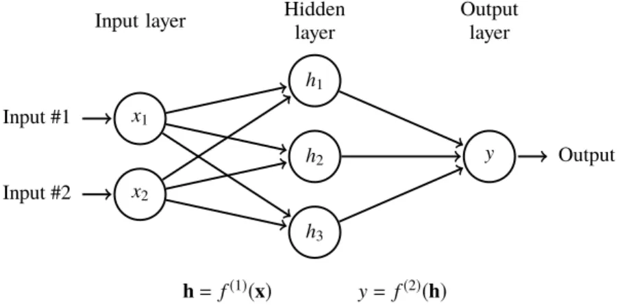
An example of a simple multilayer perceptron can found in Figure 2.5. A multilayer perceptron contains always an input layer, an output layer and one or more hidden layers, i.e. two or more perceptrons chained together. The number of layers is referred as the depth of the network, which is the origin of the term "deep learning". Input layer is just a collection of input values and thus not a perceptron like the other two layers. Our example has a vector valued inputx=[x1,x2]⊤, hidden layerh=[h1,h2,h3]⊤and an output value y.
In the graph the variables are denoted with nodes and their relations are indicated by the edges.
x1 Input #1 x2 Input #2 h1 h2 h3 y Output Hidden layer
Input layer Output
layer
h=f(1)(x) y=f(2)(h)
Figure 2.5. A simple multilayer perceptron.
This network can represented as a chain of functions f(x)= f(2)(f(1)(x)), where the hidden layer is represented by the equationh= f(1)(x)and the output layer by y= f(2)(h). The functions f(1)and f(2)are defined as
f(1)(x)=W⊤x+b (2.32)
f(2)(h)=w⊤h+c, (2.33)
whereWis a 2×3 matrix containing the weights of the hidden layer, vectorb=[b1,b2,b3]⊤
contains the biases for the hidden layer, vectorw=[w1,w2,w3]⊤ contains the output layer
weights andcis the output bias. Together these parametersθθθ={W,w,b,c}are the trainable parameters of this network, and we will use the notation f(x;θθθ)to indicate the models dependency on the parameters, when referring to the network.
2.4.1
Activation layers
Neural networks are known for their ability to approximate nonlinear functions, but the above example consists of only linear functions. No matter how many linear functions we chain to together, the model will stay linear. Thus we need to introduce some nonlinearity to the model, which is achieved using activation functions. The most common activation function in modern neural networks is the rectified linear unit (ReLU) [19, p. 171], which is defined as
g(z)=max{0,z}. (2.34)
The activation function is used in the hidden layers to modify the output of the nodes. In the above example we would utilize it after the function f(1)so that the model becomes
f(x)= f(2)(g(f(1)(x))).
Earlier neural networks used the sigmoid, or logistic, activation function, which is defined as
σ(x)= 1
Sigmoid function’s output range is(0,1), and it saturates strongly negative values to zero and strongly positive values to one. This saturation leads to problem known as vanishing gradients with deeper networks. Vanishing gradients can be mitigated by using ReLU activation instead in the hidden layers, but sigmoid function is still useful as the output unit in classifier networks. For regression tasks like SR the best choice is using linear output unit.
2.4.2
Loss functions
Although the goal of training a neural network is maximizing some performance metric (in our case PSNR and SSIM), the same metric used in performance comparison is not typically used for steering the training process. In some cases it could be possible, at least with some minor modifications to the metric, but it still might not feasible. The metric used in the training process is called the loss function (or cost function), and the goal of the process is to minimize it on the training data. In this thesis the loss function refers to a loss calculated on a single example, and the cost function refers to loss calculated on the whole dataset or specific subset of it, although in some literature they are used interchangeably. Given a loss function L(y,ˆ y), where ˆy= f(x)is the network output andyis the training target corresponding to the inputx, the loss function output is a scalar with lower values corresponding to greater similarity between vectorsyand ˆy. The only other requirement for the loss funtion is that it is differentiable over ˆy, as the parameter updates done during the training are based on the gradient of the loss function.
The most common loss function used in image processing tasks like SR, is theℓ2 loss,
which is defined as the square ofℓ2norm of the differencey−yˆ
Lℓ2(y,yˆ )= ∥y−yˆ∥22. (2.36)
This loss function is essentially the sum of squared errors, thus minimizing it minimizes also MSE and maximizes PSNR. This makes it an intuitive choice for maximizing PSNR, but it has been recently shown to be a suboptimal choice.
Zhao et al. [68] compared the performance of models trained using different loss functions in three different image restoration tasks: joint demosaicking and denoising, JPEG deblocking, and super-resolution. They discovered that models optimized with the closely relatedℓ1
loss
Lℓ1(y,yˆ )= ∥y−yˆ∥1 (2.37)
produced better results MSE-wise than otherwise identical models trained withℓ2loss.
They attributed this difference toℓ2loss’ higher tendency to get stuck in a local minimum
during training. Using combination of both losses Zhao et al. were able to decrease the MSE even further, with best results given by first usingℓ1and then finalizing withℓ2.
The motivation of Zhao et al. was to increase the perceived quality of the images, as MSE and its derivatives have been known to be poor estimates of perceived quality. Thus they tested also loss functions based on the SSIM metric and proposed a hybrid approach using a mixture ofℓ1and SSIM loss functions. There has been also perceptual loss functions that
utilize high level features extracted from neural networks trained for image classification. The distance between the features extracted from super-resolved image and the features from the target image is used instead of per-pixel differences. This approach was first introduced for texture synthesis [14, 15], but it has been also employed for super-resolution [28, 35, 49].
As we are not interested in the networks performance on a single training example, we introduce the total cost function
J (θθθ;X,Y)= 1 m m−1 ∑ i=0 L(f(xi;θθθ),yi), (2.38)
whereXandYare matrices containing allmtraining example pairsxiandyi[19, p. 149]. Ultimately we would want to minimize
J (θθθ)=E(x,y)∼pdataL(f(x;θθθ),y), (2.39) which is the expected cost of anyxandybelonging to the data-generating distributionpdata [19, p. 272]. As the actual distribution is typically unknown, we can only estimate the cost
J (θθθ)with the equation 2.39.
The difference between the network output and the target is not always the only thing we want to minimize, and many times it beneficial to keep the trainable parametersθθθ at relatively low values. This limits the model’s capacity and thus lowers its tendency to overfit. This is achieved by introducing a parameter norm penaltyΩ(θθθ)to the total cost function
˜
J (θθθ;X,Y)= J (θθθ;X,Y)+αΩ(θθθ), (2.40)
whereαis a hyperparameter affecting the strength of the norm penalty. This regularized total cost ˜J will be the target of optimization and minimizing it requires balancing the loss L and the norm penalty Ω. The most widely used norm penalties are the ℓ2
penaltyΩℓ2(θθθ)= ∥θθθ∥2and theℓ1penaltyΩℓ1(θθθ)=∥θθθ∥1[19, p. 227–232]. The penalty is
typically calculated separately for every layer of the network and theαparameter can be set individually for every layer. Parameter norm penalty is one form of regularization, which refers to any modifications done to the model to prevent overfitting [19, p. 224]. The above mentioned norm penalties are the most widespread regularization methods, and are often referred as justℓ2andℓ1regularization.
2.4.3
Optimization
Although the cost J (θθθ;X,Y)is easy to calculate, finding the optimal parameter values
θθθ0=arg min
θθθ
is practically impossible due to the high nonlinearity of a typical neural network. The cost function will be non-convex with numerous local minima, and the goal of the optimization is to find a minimum that is low enough for the task at hand. This is done using the gradient descent algorithm, which iteratively updates the parametersθθθby choosing
θθθ′=θθθ−ϵ∇
θθθJ (θθθ;X,Y) (2.42)
as the next set of parameter values after each update. The scalar ϵ is the learning rate parameter affecting the speed of descent and ∇θθθJ (θθθ;X,Y) is the gradient of the cost function. The parameter values are updated towards the negative gradient, with the norm of the gradient and the learning rate dictating the magnitude of the updates.
The calculation of the gradient
∇θθθJ (θθθ;X,Y)= 1 m m−1 ∑ i=0 ∇θθθL(f(xi;θθθ),yi) (2.43)
has to be done for each update step, and its computational complexity isO(m). With datasets large enough to be useful, the cost of this operation becomes prohibitively high. As this cost function is only an estimate of the ideal costJ (θθθ), we can estimate the gradient
∇θθθJ (θθθ) with a smaller subset of m′ training samples. This subset is called minibatch and the number of samplesm′is referred as the batch size. The estimated gradient then becomes g= 1 m′ m′−1 ∑ i=0 ∇θθθL(f(xi;θθθ),yi), (2.44)
and the samples in the minibatch are redrawn from the training set for every update step. Every sample will be used only once, until the whole training set has been processed and the cycle begins again. This cycle is called epoch, and the number of epochs tells us how many times the model has seen each individual training sample.
This minibatch gradient descent algorithm is often called stochastic gradient descent (SGD), although originally that term referred only to the extreme case ofm′=1 [19, p. 275–276].
SGD, or some variation of it, is used for optimization in practically every modern neural network. Algorithm 2.1 illustrates how a simple version of SGD could be implemented. The learning rateϵk is set separately for each iterationk, as in practical scenarios it has to be decreased as the training progresses. This is due to the noisy gradient estimate used in SGD, which does not converge to zero even if a minimum is reached. [19, p. 290–291] A common extension to SGD is momentum, which is meant to accelerate the learning process. It is inspired by its physical namesake and introduces a variablevwhich represents velocity. The velocity defines the parameter update direction and magnitude, and the velocity is computed at each iteration from the current gradient and previous velocity. The algorithm 2.1 can be extended with momentum by changing the update step tov←αv−ϵkg
Require: Learning rate scheduleϵ0,ϵ1,. . .
Initialize parametersθθθ
k←0
whilestopping criterion not metdo
Sample a minibatch ofm′examplesxiandyifrom the training set. Compute the gradient estimate: g← m1′
∑m′−1
i=0 ∇θθθL(f(xi;θθθ),yi)
Update the parameters: θθθ←θθθ−ϵkg k←k+1
end while
Algorithm 2.1. Stochastic gradient descent
Learning rate is one of the most difficult hyperparameters to set, and its effects on the model performance are significant [19, p. 302]. A single learning rate for every parameter is rarely an optimal choice, as the cost function is typically sensitive to some directions in the parameter space and less sensitive to others. This has lead development of adaptive optimizers, which automatically alter the learning rate during the training process separately for every parameter. Common adaptive algorithms are for example AdaGrad by Duchi et al. [8], and Adam by Kingma and Ba [32].
With all gradient based optimizers, the calculation of the actual gradient ∇θθθL is done with an algorithm known as back-propagation. It based on the chain rule of calculus, which states that given functions f :R→Randg:R→R, and scalars x, z=g(x)and
y= f(z)= f(g(x)), the derivative of yoverxcan be calculated as
dy dx = dy dz dz dx. (2.45)
This can be easily extended to multidimensional cases. Given functions f :Rn →R andg:Rm →Rn, vectorsx∈Rm and z=g(x), and scalar y= f(z)= f(g(x)), the partial derivative of ybecomes ∂y ∂xi = n−1 ∑ j=0 ∂y ∂zj ∂zj ∂xi . (2.46)
This can be written in vector notation as
∇xy= (∂z
∂x
)⊤
∇zy, (2.47)
where ∂∂xz is then×mJacobian matrix ofg. [19, p. 201–203]
Equation 2.47 forms the basis of the back-propagation algorithm. It shows that to calculate the gradient of variablex, we can multiply a Jacobian matrix ∂∂xz with a gradient∇zy. In the back-propagation algorithm this product is calculated for each layer of a neural network recursively, starting from the output and progressing backwards to the input layer. The gradients of the later layers are used to calculate the gradients of earlier layers, i.e. the gradient is propagated backwards in the network. The derivation of the complete algorithm is outside the scope of this thesis, and we refer to the book Deep Learning by Goodfellow et al. [19] for further information on the topic.
2.4.4
Convolutional layers
Fully connected neural networks have a few limitations that make them poorly suitable for image processing tasks, but those limitations can be overcome using convolutional layers. Fully connected networks are limited fo fixed size inputs and outputs, and they become computationally heavy with large input and output sizes, as each node of a layer is connected to every node of the next layer. Withninputs andmoutputs, the number of trainable parameters of a fully connected layer becomesnm(or(n+1)mif bias parameters are counted). [19, p. 330]
Convolutional layers work similarly to traditional discrete convolution, and thus the number parameters stays constant regardless of the input size, as the same set of filter coefficients is used for every input segment. In addition to enabling arbitrary-sized inputs and lowering the number of parameters, convolutional layers make the network spatially invariant. This is desirable in super-resolution and similar image processing tasks as the input patch should be processed identically regardless of its location in the input image. [19, p. 331–335] A simple one-dimensional convolutional layer is shown in Figure 2.6(a). Its input is vector
x=[x0,x1,x2,x3,x4]⊤, and its output is vectory=[y0,y1,y2]⊤ whose values are defined by
the equation yi= 2 ∑ j=0 wjxi+j+c, (2.48)
wherewjare the coefficients of the filter vectorw=[w0,w1,w2]⊤andcis the bias parameter.
With a filter of lengthn, the output will always ben−1 shorter than the input, unless some
form of input padding is used. Figure 2.6(b) shows a convolutional layer with the same input and filter, but with zero-padding used in the input. [19, p. 342–343]
The output size can be kept identical to the input size by using zero-padding, but sometimes it is desirable to change the data size inside the network. Typical image classification networks decrease the size deliberately with pooling layers to introduce invariance to small input translations, and to lower the computational costs [19, p. 335–339]. Pooling is less useful in super-resolution and thus outside scope of this thesis.
Although super-resolution aims to increase the resolution of images, some SR networks utilize also donwsampling layers in their architecture [21]. Downsampling can be done with strided convolution, which is illustrated in Figure 2.7. Convolution with a stride k
progresses in steps ofk elements over the input, and produces output of length kj, when input length is j and input padding used. Strided convolution can also thought as normal convolution, where all but everykth output value is discarded.
If we want to increase the size with a factor of k instead of decreasing it, we can use convolution with a stride of 1k. This scheme is also known as deconvolution, transposed convolution, sub-pixel convolution, and numerous other names [51], but we will call it
x1 x2 x3 x4 x5 y1 y2 y3
(a)No input padding
x1 x2 x3 x4 x5 0 0 y1 y2 y3 y4 y5 (b)Zero-padding
Figure 2.6. Two versions a simple one-dimensional convolutional layer with input length of 5 and filter length of 3. The first one has no input padding which leads to smaller sized
output and the second one uses zero-padding to preserve the input size in the output.
x1 x2 x3 x4 x5 x6 0 y1 y2 y3 (a)Stride 2 x1 x2 x3 0 0 0 0 0 y1 y2 y3 y4 y5 y6 (b)Deconvolution (stride12)
Figure 2.7. Two examples of one-dimensional convolution where data size changes deliberately. First one shows convolution with stride 2, which halves the size. Second one
shows deconvolution with factor of 2 (stride 12), which doubles the size of input.
deconvolution from now on. The term sub-pixel convolution is used for a closely related scheme, which will be explained later in more detail. Deconvolution can be exemplified as normal convolution, where the input vector has zeros added between every input element. This is visualized in Figure 2.7(b) with filter length of 3, stride12, and zero-padded input.
Until now we have discussed only one-dimensional inputs, outputs, and filters, but images are usually two-dimensional and represented as matrices. In the case of color images we have normally three channels for every pixel, and we need to use three-dimensional arrays to represent them. To extend the concept of vectors and matrices to arbitrary number of dimensions, tensors are typically used [19, p.31]. Further discussion of the tensor theory is beyond the scope of this thesis, but we will use tensors to describe multi-dimensional arrays in the rest of this chapter.
All of the one-dimensional examples we have discussed thus far can be easily extended to multiple dimensions. Images are typically arranged inton×m×ctensors, wherenis the number of number rows,mis the number of columns andcis the number color channels. With grayscale images c=1, but they are still processed like other three-dimensional
tensors. A convolutional layer at the input of a image processing network would have filter kernel ofk1×k2×c, wherek1andk2hyperparameters define the filter size. Although the
filter has a third dimension of lengthc, this is still considered two-dimensional convolution. The filter length in third dimension is set as the same as the input’s third dimension, and the output will be two-dimensional.
Each hidden convolutional layer will typically have f unique filter kernels, and the layer output is arranged as an×m× f tensor, assuming that input size isn×m×cand padding is used. Thus the next layer will have filter size of k1×k2× f. The output layer will have
the number of filters set according to the desired number color channels.
Figure 2.8 illustrates a two-dimensional case of deconvolution, with a 4×4×1 input tensor, 4×4×1 filter kernel, stride of 12, and zero-padding. The output is a 8×8×1 tensor. White
squares are used to depict the pixels of the input image, gray squares are the zeros used for padding, and colored squares illustrate the connection between output pixels and the filter coefficients used to calculate those pixels.
Figure 2.8. Two-dimensional deconvolution with stride 12 [51].
Figure 2.9 shows an alternative way to implement similar upscaling operation inside a convolutional network. This method was introduced by Shi et al. [50, 51] and they named it "efficient sub-pixel convolution", but we will refer to it as just sub-pixel convolution. The input and outputs are the same size as in the previous example, but the filter is different. Instead of a single filter, four individual kernels of size 2×2×1 are used with stride 1,
Figure 2.9. Two-dimensional sub-pixel convolution with scaling factor of 2 [51].
in the way illustrated by the color coding. In the general case this transforms an×m×cr2
sized tensor to sizern×rm×c, wherer is the scaling factor andcis the number of color channels.
In this simple example case the difference between these two methods is purely imple-mentational, as both methods use identical number of filter coefficients to produce and identically sized output. However, Shi et al. [51] showed that their sub-pixel convolution allows for greater flexibility with the filter sizes used, and is easier to implement efficiently. There are also other modifications and extensions to convolutional layers, but most of the super-resolution networks utilize only normal convolutional layers, and the above mentioned upsampling convolutions. Concrete examples of those networks are given in Section 3.5.
3. SUPER-RESOLUTION
Super-resolution (SR) aims to produce an high resolution (HR) image, given one or more low resolution (LR) images as input. In contrast to simple interpolation techniques like the ones described in Section 2.1, SR methods aim at recovering or estimating the information missing from the low-resolution image. There are multiple ways to approach the problem and SR algorithms can be classified in numerous ways. The simplest way is to classify them either single image SR (SISR) or multi-image SR (MISR), based on the number of low resolution input images used. MISR tackles the problem with multiple different images depicting the same scene, with each image having different sub-pixel alignments (translation, rotation etc.), different scales, different blurring, or other similar variations between them. As a single low resolution image could have been produced by scaling down infinite number of different high resolution images,


![Figure 3.1. The network structure of SRCNN [6].](https://thumb-us.123doks.com/thumbv2/123dok_us/34120.2504797/41.892.169.804.106.334/figure-the-network-structure-of-srcnn.webp)
![Figure 3.3. The network structure of ESPCN for scale factor of r [50].](https://thumb-us.123doks.com/thumbv2/123dok_us/34120.2504797/42.892.183.801.614.774/figure-network-structure-espcn-scale-factor-r.webp)
