Object-Based Supervised Machine Learning Regional-Scale Land-Cover Classification Using High Resolution Remotely Sensed Data

(1)

Graduate Theses, Dissertations, and Problem Reports 2019

Object-Based Supervised Machine Learning Regional-Scale

Land-Cover Classification Using High Resolution Remotely Sensed Data

Cover Classification Using High Resolution Remotely Sensed Data

Christopher A. Ramezan

West Virginia University, [email protected]

Follow this and additional works at: https://researchrepository.wvu.edu/etd

Part of the Geographic Information Sciences Commons, Physical and Environmental Geography

Commons, Remote Sensing Commons, Spatial Science Commons, and the Theory and Algorithms Commons

Recommended Citation Recommended Citation

Ramezan, Christopher A., "Object-Based Supervised Machine Learning Regional-Scale Land-Cover Classification Using High Resolution Remotely Sensed Data" (2019). Graduate Theses, Dissertations, and Problem Reports. 3876.

https://researchrepository.wvu.edu/etd/3876

This Dissertation is protected by copyright and/or related rights. It has been brought to you by the The Research Repository @ WVU with permission from the rights-holder(s). You are free to use this Dissertation in any way that is permitted by the copyright and related rights legislation that applies to your use. For other uses you must obtain permission from the rights-holder(s) directly, unless additional rights are indicated by a Creative Commons license in the record and/ or on the work itself. This Dissertation has been accepted for inclusion in WVU Graduate Theses, Dissertations, and Problem Reports collection by an authorized administrator of The Research Repository @ WVU. For more information, please contact [email protected].

(2)

Object-Based Supervised Machine Learning Regional-Scale Land-Cover Classification Using High Resolution Remotely Sensed Data

Christopher A. Ramezan

Dissertation submitted to the Eberly College of Arts and Sciences at West Virginia University

in partial fulfillment of the requirements for the degree of

Doctor of Philosophy in

Geography

Timothy A. Warner, Ph.D., Chair Jamison Conley, Ph.D.

Gregory Elmes, Ph.D. Rick Landenberger, Ph.D. Ramesh Sivanpillai, Ph.D.

Department of Geology and Geography

Morgantown, West Virginia 2019

Keywords: Remote Sensing, GEOBIA, NAIP, LIDAR, High Resolution, Machine Learning, Supervised Classification, Regional-Scale, Land-Cover Mapping

(3)

Abstract

Object-Based Supervised Machine Learning Regional-Scale Land-Cover Classification Using High Resolution Remotely Sensed Data

Christopher A. Ramezan

High spatial resolution (HR) (1m – 5m) remotely sensed data in conjunction with supervised machine learning classification are commonly used to construct land-cover classifications. Despite the increasing availability of HR data, most studies investigating HR remotely sensed data and associated classification methods employ relatively small study areas. This work therefore drew on a 2,609 km2_{, regional-scale} study in northeastern West Virginia, USA, to investigates a number of core aspects of HR land-cover supervised classification using machine learning. Issues explored include training sample selection, cross-validation parameter tuning, the choice of machine learning algorithm, training sample set size, and feature selection. A geographic object-based image analysis (GEOBIA) approach was used. The data comprised National Agricultural Imagery Program (NAIP) orthoimagery and LIDAR-derived rasters. Stratified-statistical-based training sampling methods were found to generate higher classification accuracies than deliberative-based sampling. Subset-based sampling, in which training data is collected from a small geographic subset area within the study site, did not notably decrease the classification accuracy. For the five machine learning algorithms investigated, support vector machines (SVM), random forests (RF), k-nearest neighbors (k-NN), single-layer perceptron neural networks (NEU), and learning vector quantization (LVQ), increasing the size of the training set typically improved the overall accuracy of the classification. However, RF was consistently more accurate than the other four machine learning algorithms, even when trained from a relatively small training sample set. Recursive feature elimination (RFE), which can be used to reduce the dimensionality of a training set, was found to increase the overall accuracy of both SVM and NEU classification, however the improvement in overall accuracy diminished as sample size increased. RFE resulted in only a small improvement the overall accuracy of RF classification, indicating that RF is generally insensitive to the Hughes Phenomenon. Nevertheless, as feature selection is an optional step in the classification process, and can be discarded if it has a negative effect on classification accuracy, it should be investigated as part of best practice for supervised machine land-cover classification using remotely sensed data.

(4)

iii

Dedication

(5)

iv

Chapter 1 - Introduction

1. Background

High-spatial resolution (HR) (1m – 5m) earth observation datasets can be used to develop land-cover classifications of the earth’s surface to monitor our ever-changing landscape. Over the past few decades, starting with the launch in late 1999 of IKONOS, the first

commercially available spatial HR earth observation satellite, HR remotely sensed data has become increasingly available for public use. However, HR remotely sensed data are rarely analyzed on large, regional or national scales. Regional-scale in this context simply refers to a large, multi-county study area, rather than definitions used in disciplines such as landscape ecology or ecology.

Typically, regional- or national-scale land-use/land-cover (LULC) maps are constructed from medium- or coarse-spatial resolution remotely sensed data. For example, the 2011 National Land Cover Dataset (NLCD) is based on medium resolution Landsat data, providing a 30m land cover dataset over the contiguous United States (Homer et al., 2015). Global-scale datasets, such as the Vegetation Continuous Fields (VCF) dataset, constructed from MODIS imagery, typically have an even coarser spatial resolution, such as 250 m or 1 km. While

medium or coarse-spatial resolution datasets can be useful, the scale is inappropriate for studies that require finer spatial detail (Li and Shao, 2014), such as urban feature extraction

(Benediktsson et al., 2003; Kong et al., 2006; Taubenböck et al., 2010), tree crown mapping (Karlson et al., 2014), forest structural parameter estimation (Galidaki, et al., 2016; Wolter et al., 2009) and small-area site-specific crop management (SSCM) or precision agriculture mapping (Mulla, 2013).

(9)

2

Despite advances in information technology platforms, and increasing availability of HR remotely-sensed datasets, large-scale HR land-cover classifications remain rare (Ma et al., 2017; O’Neil-Dunne et al., 2014). The lack of large-scale (large-scale in this context meaning large geographic areas) land-cover analyses is likely due in part to the relatively large data volume of HR datasets compared to coarser resolution datasets covering the same area. To partially assist with remediating data volume and processing issues with large-scale HR datasets, Geographic Object-Based Image Analysis (GEOBIA) approaches have been suggested for conducting large-scale HR land-cover classifications (Demarchi et al., 2017; Li and Shao, 2014; Lubker and Schaab, 2010).

GEOBIA is a relatively recent paradigm in remote sensing which has several potential advantages over traditional pixel-based approaches when analyzing HR remotely sensed data (Arvor et al., 2013; Blaschke, 2010; Blaschke et al., 2014; Hay and Castilla, 2008; Hay and

Blaschke, 2010). GEOBIA approaches can mitigate some of the technical challenges in classifying HR data through the grouping of heterogeneous pixels into discrete image-objects. Rather than having to analyze and classify each pixel individually, segmented groups of pixels, called image-objects, form the base unit of analysis, thus reducing the overall number of data units and in turn reducing the processing demands (Zhang et al., 2007). In addition, GEOBIA approaches can help to reduce the effects of high intra-class spectral variability or “salt and pepper” texture, which is a commonly encountered obstacle in HR classifications of remotely sensed data (Blaschke, 2010).

Object-based analyses of HR remotely sensed data have been conducted for a variety of applications, such as land-use/land-cover mapping (Antonarakis, et al., 2008; Elhadi et al., 2014; Im et al., 2013; Lu and Weng, 2007; Liu and Xia, 2009; Tehrany et al., 2014; Walker and Blaschke, 2006; Zhou et al., 2008) tree-canopy mapping (Chen and Hay, 2011; O’Neil-Dunne et al., 2014;

(10)

3

Machala and Zejdova, 2014), mine-reclaimed land mapping (Maxwell and Warner, 2015), hydrological mapping (Demarchi et al., 2017), bathymetric mapping (Diesing et al., 2014; Diesing et al., 2016; Lacharité et al., 2015), and acoustic remote sensing (Hill et al., 2014), among others. While GEOBIA has become a popular method for analyzing remotely sensed datasets, a majority of basic and applied object-based analyses using HR data reported in the literature are also conducted on geographically small areas (Ma et al., 2017).

Supervised machine learning algorithms are a popular method for constructing land-cover classifications in GEOBIA and remote sensing analyses in general. Supervised machine learning classifiers are mathematical algorithms that use pre-labeled training examples to infer a function, which can be applied to classify new unseen examples. Machine learning has become increasingly popular in a variety of fields, such as biomedical science (Cao et al., 2018) and automotive engineering (Huval et al., 2015). Machine learning methods are particularly attractive to remote sensing scientists due to the typical high data volume and complexity of remotely sensed data.

While many core methodological themes and issues in GEOBIA-based supervised machine learning land-cover classifications such as sample selection, cross-validation, machine learning algorithms, and classification optimization, have been widely examined within the literature, these concepts are rarely, if ever investigated on large, HR regional-area datasets.

This work therefore seeks to investigate methods for developing large area, supervised

machine learning regional-scale object-based land-cover classifications of HR remotely sensed

data. As traditional remote sensing methods applied to large datasets may be expensive in

terms of human and computer effort, this work examines several core HR remote sensing methodological questions, such as sample selection, model cross-validation, supervised machine

(11)

4

learning algorithms, and feature optimization at large, regional scales. In addition, this work provides a practical approach for developing applied regional-scale HR land-cover classifications datasets using an object-based approach.

2. Research Themes and Aims

Through investigation of the development of regional-scale object-based high-resolution land-cover classifications, this dissertation addresses the following research questions: 1. As sample selection is a critical component of conducting supervised machine learning

classifications, how do various aspects of sample acquisition processes such as sample size, sample location, and sampling technique affect the accuracy of supervised regional-scale land-cover classifications of HR remotely sensed data?

2. Cross-validation tuning is often used to optimize parameter selection in supervised machine learning classifiers. While a variety of cross-validation tuning methods are commonly used in remote sensing analyses, they are rarely compared. Do different cross-validation tuning methods provide inherent advantages for improving supervised classifier performance of regional-scale HR remotely sensed data?

3. As various supervised machine learning methods are commonly employed for constructing land-cover classifications of remotely sensed data, how do the following supervised machine learning classifiers: Support Vector Machine (SVM), Random Forests (RF), k-Nearest

Neighbors (k-NN), Neural Networks (NEU), and Learning Vector Quantization (LVQ) perform when constructing regional-scale HR land-cover maps?

(12)

5

4. High dimensional remotely sensed datasets can contain highly correlated or irrelevant bands (or features) that can negatively affect the performance of supervised machine learning classifiers, a problem known as the curse of dimensionality or the Hughes Phenomenon (Hughes, 1968). Automated feature selection approaches have therefore been suggested for optimizing the feature space of training sets, and reducing the data dimensionality. This work investigates if recursive feature elimination improves classifier performance when applied to large, regional-scale HR remotely sensed datasets and using three supervised machine learning classifiers: Support Vector Machines (SVM), Random Forests (RF), and Neural Networks (NEU).

(13)

6

3. Objectives and Structure

This dissertation consists of three main chapters, each written as a stand-alone article, with its own experimental design. Additionally, an introduction chapter that explains the overall context of the work, and a conclusion chapter that summarizes and reflects on the findings of the three articles, are included.

Chapter 2 focuses on research question one, examining how the performance of

support vector machines (SVM) supervised regional-scale HR land-cover classification is affected by training sets that vary in size, acquisition location, and collection method. In addition, chapter 2 also examines the second question in a comparison of cross-validation tuning methods in a regional-scale land-cover classification of HR remotely sensed data.

Chapter 3 focuses on the first and third research questions by investigating how training samples of varying size acquired from differing geographic regions affect the performance of several different supervised machine learning algorithms when applied to a regional-scale HR land-cover classification.

Chapter 4 focuses on the first and fourth research questions by examining how feature selection techniques such as can be used to improve performance of regional-scale HR

(14)

7

4. References

Arvor, D., L. Durieux, S. Andrés, and Laporte, M.A. (2013). Advances in Geographic Object-Based Image Analysis with Ontologies: A Review of Main Contributions and Limitations from a Remote Sensing Perspective. ISPRS Journal of Photogrammetry and Remote Sensing, 82: 125–137.

doi:10.1016/j.isprsjprs.2013.05.003

Antonarakis, A. S., Richards, K. S., Basington, J. (2008). Object-based land cover classification using airborne LiDAR. Remote Sensing of Environment. 112(6). 2988-2998.

https://doi.org/10.1016/j.rse.2008.02.004.

Benediktsson, J. A., Pesaresi, M., Amason, K. (2003). Classification and feature extraction for remote sensing images from urban areas based on morphological transformations. IEEE Transactions of Geoscience and Remote Sensing. 41(9). 1940-1949. DOI: 10.1109/TGRS.2003.814625.

Blaschke, T. (2010). Object based image analysis for remote sensing. ISPRS Journal of Photogrammetry and Remote Sensing, 65 (1), 2-16. http://dx.doi.org/10.1016/j.isprsjprs.2009.06.004.

Blaschke, T., Hay, G. J., Kelly, M., Lang, S., Hofmann, P., Addink, E., . . . Tiede, D. (2014). Geographic Object-Based Image Analysis – Towards a new paradigm. ISPRS Journal of Photogrammetry and Remote Sensing, 87, 180-191. doi:10.1016/j.isprsjprs.2013.09.014.

Cao, C., Liu, F., Tan, H., Song, D., Shu, W., Li, W., Zhou, Y., Bo, X., Xie, Z. (2018). Deep Learning and Its Applications in Biomedicine. Genomics, Proteomics & Bioinformatics. 16(1). 17-32.

https://doi.org/10.1016/j.gpb.2017.07.003.

Chen, G., and Hay, G. J. (2011). An airborne lidar sampling strategy to model forest canopy height from Quickbird imagery and GEOBIA. Remote Sensing of Environment. 115(6). 1532-1542.

Demarchi, Luca., Bizzi, Simone., Piegay, Herve. (2017). Regional hydromorphological characterization with continuous and automated remote sensing analysis based on VHR imagery and low-resolution LiDAR data. Earth Surface Processes and Landforms. 42(3). 531-551. DOI: 10.1002/esp.4092.

Diesing, M., Green, S. L., Stephens, D., Lark, R. M., Stewart, H. A., and Dove, D. (2014). Mapping seabed sediments: Comparison of manual, geostatistical, object-based image analysis and machine learning approaches. Continental Shelf Research. 84 (1). 107-119. https://doi.org/10.1016/j.csr.2014.05.004. Diesing, M., Mitchell, P., and Stephens, D. (2016). Image-based seabed classification: What can we learn from terrestrial remote sensing? ICES Journal of Marine Science. 73(10). 2425-2441.

Elhadi, A., Mutanga, O., Odindi, J., and Abdel-Rahman, E. M. (2014). Land-use/cover classification in a heterogeneous coastal landscape using RapidEye imagery: evaluating the performance of random forest and support vector machine classifiers. International Journal of Remote Sensing 35(10). 3440-3458.

https://doi.org/10.1080/01431161.2014.903435.

Galidaki, G., Zianis, D., Gitas, I., Radoglou, K., Karathanassi, V., Tsakiri-Strai, M. (2016). Vegetation biomass estimation with remote sensing: focus on forest and other wooded land over the Mediterranean ecosystem. International Journal of Remote Sensing. 38(7). 1940-1966.

(15)

8

Hay, G. J., and Castilla, G. (2008). Geographic Object-Based Image Analysis (GEOBIA): a new name for a new discipline. In T. Blaschke, S. Lang, G. Hay (EDs.) Object-Based Image Analysis. Springer, Heilderberg, Berlin, NY (2008). 78-85.

Hill, N. A., Lucieer, V., Barrett, N. S., Anderson, T. J., Williams, S. B. (2014). Filling the gaps: Predicting the distribution of temperate reef biota using high resolution biological and acoustic data. Estuarine, Coastal and Shelf Science. 147 (20). 137–147. https://doi.org/10.1016/j.ecss.2014.05.019.

Homer, C.G., Dewitz, J.A., Yang, L., Jin, S., Danielson, P., Xian, G., Coulston, J., Herold, N.D., Wickham, J.D., and Megown, K. (2015). Completion of the 2011 National Land Cover Database for the

conterminous United States-Representing a decade of land cover change information. Photogrammetric Engineering and Remote Sensing, 81(5), 345-354.

Hughes, G. (1968). On the mean accuracy of statistical pattern recognizers. IEEE Transactions on Information Theory. 14(1). 55-63. DOI: 10.1109/TIT.1968.1054102.

Huval, B., Wang, T., Tandon, S., Kiske, J., Song, W., Pazhayampallil, J., Andriluka, M., Rajpurkar, P., Migimatsu, T., Cheng-Yue, R., Mujica, F., Coates A., and Ng, A. Y. (2015). An Empirical Evaluation of Deep Learning on Highway Driving. arXiv: Robotics. 1-7. https://arxiv.org/pdf/1504.01716v1.pdf.

Im, J., Jensen, J. R., and Hodgson, M. E. (2013). Object-Based Land Cover Classification Using High-Posting-Density LiDAR Data. GIScience & Remote Sensing. 45 (2). 209-228.

https://doi.org/10.2747/1548.1603.45.2.209.

Karlson, M., Reese, H., and Ostwald, M. (2014). Tree Crown mapping in Managed Woodlands (Parklands) of Semi-Arid West Africa Using WorldView-2 Imagery and Geographic Object Based Image Analysis.

Sensors. 14(12). 22643-22669. DOI: 10.3390/s141222643.

Kong, Chunfang., Xu, Kai., Wu, Chonglong. (2006). Classification and Extraction of Urban Land-Use Information from High-Resolution Image Based on Object-Multi-features. Journal of China University of Geosciences. 17(2). 151-157. https://doi.org/10.1016/S1002-0705(06)60021-6.

Lacharité, M., Metaxas, A., and Lawton P. (2015). Using object-based image analysis to determine seafloor fine-scale features and complexity. Limnology and Oceanography: Methods. 13. 553–567. http://doi.wiley.com/10.1002/lom3.10047

Li, Xiaoxiao and Shao, Guofan (2014). Object-Based Land-Cover Mapping with High Resolution Aerial Photography at a County Scale in Midwestern USA. Remote Sensing. 6. 11372-11390.

doi:10.3390/rs61111372.

Lu, D., Weng, Q. (2007). A survey of image classification methods and techniques for improving classification performance. International Journal of Remote Sensing, 28. 823-870.

Lubker, T. and Schaab, G. (2010). A Work-flow design for large-area multilevel GEOBIA: Integrating statistical measure and expert knowledge. In: ISPRS Proceedings (digital) of Geographic Object-Based Image Analysis (GEOBIA 2010), Vol. XXXVIII-4/C7, 29 June – 2 July 2010, Ghent (Belgium); ed. by Addink, E.A. & F.M.B. Van Coillie.

Liu, D., and Xia, F. (2010). Assessing object-based classification: advantages and limitations. Remote Sensing Letters. 2010(4). 187-194. https://doi.org/10.1080/01431161003743173.

(16)

9

Ma, L., Li, M., Ma, X., Cheng, K., Du, P., Liu Y. (2017). A review of supervised object-based land-cover image classification. ISPRS Journal of Photogrammetry and Remote Sensing. 130(2017). 277-293.

https://doi.org/10.1016/j.isprsjprs.2017.06.001.

Machala, M., and Zejova, L. (2014). Forest Mapping through Object-based Image Analysis of Multispectral and LiDAR Aerial Data. European Journal of Remote Sensing. 47(1). 117-131.

https://doi.org/10.5721/EuJRS20144708.

Maxwell. A. E., and Warner, T. A. (2015). Differentiating mine-reclaimed grasslands from spectrally similar land cover using terrain variables and object-based machine learning classification. International Journal of Remote Sensing 36(17). 4384-4410. https://doi.org/10.1080/01431161.2015.1083632. Mulla, D. J. (2013). Twenty five years of remote sensing in precision agriculture: Key advances and remaning knowledge gaps. Biosystems Engineering. 114(4). 358-371.

https://doi.org/10.1016/j.biosystemseng.2012.08.009.

O’Neil-Dunne, J., MacFaden, S., Royar, A. (2014). A Versatile, Production-Oriented Approach to High-Resolution Tree-Canopy mapping in Urban and Suburban Landscapes Using GEOBIA and Data Fusion.

Remote Sensing 6 (12), 12837-12865. https://doi.org/10.3390/rs61212837.

O’Neil-Dunne, J., MacFaden, S., Royar, A., Reis, M., Dubayah, R., Swatantran, A. (2014). An Object-Based Approach to Statewide Land Cover Mapping. ASPRS 2014 Annual Conference. Louisville, Kentucky, March 23-28, 2014. 1-6.

Taubenböck, H., Esch, T., Wurm, M., Roth, A., and Dech, S. (2010). Object-based feature extraction using high spatial resolution satellite data of urban areas. Journal of Spatial Sciences. 55(1). 117-132.

https://doi.org/10.1080/14498596.2010.487854.

Tehrany, M. S., Pradhan, B., and Jebuv, M. N. (2014). A comparative assessment between object and pixel-based classification approaches for land use/land cover mapping using SPOT 5 imagery. Geocarto International. 29(4). 351-369. https://doi.org/10.1080/10106049.2013.768300.

Walker, J. S., and Blaschke, T. (2008). Object-based land-cover classification for the Phoenix

metropolitan area: optimization vs. transportability. International Journal of Remote Sensing 29(7). 2021-2040. https://doi.org/10.1080/01431160701408337.

Wolter, P. T., Townsend, P. A., Sturtevant, B. R. (2009). Estimation of forest structural parameters using 5 and 10 meter SPOT-5 satellite data. Remote Sensing of Environment. 113(9). 2019-2036.

Zhang, L., Zhong, Y., Huang, B., Li, P. (2007). A resource limited artificial immune algorithm for

supervised classification of multi/hyper-spectral remote sensing image. International Journal of Remote Sensing. 28(7), 1665-1686.

Zhou, W., Troy, A., Grove, M. (2008). Object-based Land Cover Classification and Change Analysis in the Baltimore Metropolitan Area using Multitemporal High Resolution Remote Sensing Data. Sensors. 8(3). 1613-1636.

(17)

10

Chapter 2

Evaluation of Sampling and Cross-Validation Tuning Strategies for Regional-Scale Machine Learning Classification1

Abstract

High spatial resolution (1–5 m) remotely sensed datasets are increasingly being used to map land covers over large geographic areas using supervised machine learning algorithms. Although many studies have compared machine learning classification methods, sample selection methods for acquiring training and validation data for machine learning, and cross-validation techniques for tuning classifier parameters are rarely investigated, particularly on large, high spatial resolution datasets. This work, therefore, examines four sample selection methods—simple random, proportional stratified random, disproportional stratified random, and deliberative sampling—as well as three cross-validation tuning approaches—k-fold, leave-one-out, and Monte Carlo methods. In addition, the effect on the accuracy of localizing sample selections to a small geographic subset of the entire area, an approach that is sometimes used to reduce costs associated with training data collection, is investigated. These methods are investigated in the context of support vector machines (SVM) classification and geographic object-based image analysis (GEOBIA), using high spatial resolution National Agricultural Imagery Program (NAIP) orthoimagery and LIDAR-derived rasters, covering a 2,609 km2 regional-scale area in northeastern West Virginia, USA. Stratified-statistical-based sampling methods were found to generate the highest classification accuracy. Using a small number of training samples collected from only a subset of the study area provided a similar level of overall accuracy to a sample of equivalent size collected in a dispersed manner across the entire regional-scale dataset. There were minimal differences in accuracy for the different cross-validation tuning methods. The processing time for Monte Carlo and leave-one-out cross-validation were high, especially with large training sets. For this reason, k-fold cross-validation appears to be a good choice. Classifications trained with samples collected deliberately (i.e., not randomly) were less accurate than classifiers trained from statistical-based samples. This may be due to the high positive spatial autocorrelation in the deliberative training set. Thus, if possible, samples for training should be selected randomly; deliberative samples should be avoided.

1_{Published by MDPI in}_{Remote Sensing}_{on 18 January 2019. Available online:} https://www.mdpi.com/2072-4292/11/2/185. Ramezan, C. A., Warner, T. A., Maxwell A. E. 2019. Evaluation of Sampling and Cross-Validation Tuning Strategies for Regional-Scale Machine Learning Classification. Remote Sensing. 11(2): 185.

(18)

11

1. Introduction

With the increasing availability of high spatial resolution (HR) remotely sensed datasets (1–5 m pixels), the routine production of regional-scale HR land-cover maps has become a possibility. However, due to the large area associated with regional-scale HR remote sensing projects, the sample selection for training and assessment can be burdensome. Sampling strategies that are commonly used in remote sensing analyses involving smaller datasets may be unsuitable or impractical for regional-scale HR analyses. This is particularly true if the sampling protocol requires field observations. While much previous remote sensing research has been conducted on supervised classification sample selection methods for training [1–3] and accuracy assessments [4–7], most of these studies examine sampling methods using study sites of limited geographic extent. The limited area of these study sites is typical of classification experiments in general; Ma et al. [8] meta-reviewed over 170 supervised object-based remote sensing analyses and found that an overwhelming majority of geographic object-based image analyses (GEOBIA) studies were conducted on areas smaller than 300 ha.

This work, therefore, investigates a variety of sample selection method techniques for regional-scale land-cover classifications with large, HR remotely sensed datasets. Additionally, as the number of samples is limited in many regional studies, cross-validation for regional HR classification is also explored. Cross-validation is an approach for exploiting training and accuracy assessment samples multiple times and thus potentially improving the reliability of the results. Finally, as the acquisition of widely dispersed samples across a large region may be expensive, a sampling strategy which confines the sample selection to a small geographic subset area is also investigated. This study is conducted in the context of GEOBIA, an approach that has become increasingly popular for analyzing high-resolution remotely sensed data [8,9].

(19)

12

1.1. Background on Sample Selection in Remote Sensing

Samples in remote sensing analyses are typically collected for two purposes: training data for developing classification models and assessment or test data for evaluating the accuracy of the map product. Supervised classifiers, such as machine learning algorithms, use pre-labeled samples to train the classifier, which is then used to assign class labels to the remaining population. As the collection of training data inherently requires sampling, the strategies used for the sample selection must be carefully considered in the context of the characteristics of the dataset, classifier, and study objectives [10]. Although sample selection strategy is widely discussed in the remote sensing literature, there are a variety of opinions on almost every aspect of the sampling process. Nevertheless, there is a consensus that the size [5,7,11,12] and quality [12] of the training sample dataset, as well as the sample selection method used [5], can affect classification and accuracy assessments.

A variety of statistical (e.g., simple random and stratified random) and non-statistical (e.g., deliberative) sample selection methods have been used to collect training and testing samples for remote sensing analyses. Mu et al. [13] separated statistical-based sampling into two categories: spatial and aspatial approaches. Spatial sampling considers the spatial autocorrelation inherent in geographic data, while aspatial methods, which ignore potential spatial autocorrelation, include approaches such as simple random and stratified sampling. Although problems associated with aspatial sampling methods in remote sensing have been noted [14–16], spatial sampling methods can be complex and typically require a priori information about the population, which may be difficult or impractical to collect. While spatial sampling methods have been used in remote sensing analyses, currently they are far less

common than aspatial methods and consequently not pursued in this study.

Simple random sampling involves the purely random selection of samples and thus gives a direct estimate of the population parameters. Although random samples for image classification on average will sample each class (or stratum) in proportion to the area of that class in the map, any single random

(20)

13

sample will generally not do so. This can exacerbate the difficulty of dealing with rare classes. Some classifiers, including support vector machines (SVM), are sensitive to imbalanced training data sets, in which some classes are represented by a much smaller number of samples than other classes [17].

Stratified random sampling addresses this problem by forcing the number of samples in each stratum to be proportional to the area of the class. A variant on this method is equalized stratified random sampling, where the number of samples in each stratum is the same, irrespective of their area on the map. Equalized stratified random sampling may not be possible if some classes are so rare that the population of that class is smaller than the desired sample size. In such circumstances, a

disproportional stratified random sample may be collected, an approach in which the sizes of the strata are specified by the user and are set to intermediate values between the proportions of the areas of the classes and a simple equalized approach.

One disadvantage of all stratified approaches is that a pre-classification is needed to identify the strata. If the samples are only to be used for an accuracy assessment (and not training), then it is

possible to use the classification itself to generate the strata. However, Stehman [18] points out that if multiple classifications are to be compared and the strata are developed from just one of those classifications, the resulting accuracy statistics for the remaining maps need to be modified to account for the differences between the map used to develop the stratification and the map under

consideration. Furthermore, unlike random and stratified random sampling, equalized and

disproportional stratified random samplings produce samples that are not a direct estimate of the population. Thus, for samples generated with these methods, the accuracy estimates need adjustment to account for the class prior probabilities [19].

Deliberative sampling, in which samples are selected based on a non-random method, are also common in remote sensing. Deliberative sampling is necessary if access limitations or other issues

(21)

14

constrain the sampling. One could hypothesize that deliberative sampling might, under certain circumstances, be more effective for classifier training than random sampling. Deliberative sampling allows for the incorporation of expert knowledge into the sample selection process. For example, samples can be selected to ensure that the variability of each class is well represented. Furthermore, in SVM, only training samples that define the hyperplane separating the classes are used by the classifier. Thus, for SVM, deliberative samples selected to represent potentially spectrally confused areas may be more useful than samples representing the typical class values [20].

If in situ observations are required for sample characterization and the cost of traveling between sites is high, the spatial distribution of samples becomes a central focus. This is particularly a concern for regional-scale HR datasets. While certain innovative methods such as active learning have been

proposed to reduce sampling costs [21,22], these methods are complex to implement and are beyond the scope of this study. An alternative is localizing sample selection to a single subset area of the region of interest. Localizing sample selection to a small geographic subset area can be advantageous in large regional-scale analyses for reducing sampling costs, especially if field observations are required.

1.2. Background on Cross-Validation Tuning

A central tenet of accuracy assessment is that the samples used for training should not also be used for evaluation. A similar concern applies to the methods for selecting the user-specified

parameters required by most machine learning methods, for example, the number of trees for random forests, sigma and C values for radial basis function kernel support vector machines, and the k-distance for the k-nearest neighbors. The value of these parameters can affect the accuracy of the classification, and thus, optimizing the chosen values (sometimes called tuning) is usually required [23–26]. Tuning is generally empirical, with various values for the parameters systematically evaluated, and the

combination of values that generate the highest overall accuracy or kappa coefficient is assumed to be optimal [17,25]. Excluding training samples from the samples used for the evaluation of the candidate

(22)

15

parameter values reduces the likelihood of overtraining and thus improves the generalization of the classifier.

If the overall number of samples is small, a fixed partition of training samples into separate training and tuning samples will further exacerbate the limitations of the small sample size, since each sample is used once and for one purpose only (e.g., training). Cross-validation is an alternative approach to a fixed partition. In cross-validation, multiple partitions are generated, potentially allowing each sample to be used multiple times for multiple purposes, with the overall aim of improving the statistical reliability of the results. Examples of cross-validation methods include k-fold, leave-one-out, and Monte Carlo. Classification parameter tuning via cross-validation has been demonstrated to improve

classification accuracy in remote sensing analyses [27]. However, as with any sampling technique, it is important that the overall sample set be representative of the entire data set, otherwise the

generalizability of the supervised classifier is unknown [25].

The k-fold cross-validation method involves randomly splitting the sample set into a series of equally sized folds (groups), where k indicates the number of partitions, or folds, the dataset is split into. For example, if a k-value of ten is used, the dataset is split into ten partitions. In this case, nine of the partitions are used for training data, while the remaining one partition is used for test data. The training is repeated ten times, each time using a different partition as the test set and the remaining nine partitions as the training data. The average of the results is then reported [28].

Leave-one-out cross-validation is similar to the k-fold cross-validation except the number of folds is set as the number of samples in the sample set. This approach can be slow with very large sample sets [29].

Monte Carlo validation works on similar principles to k-fold cross-validation except that the folds are randomly chosen with replacement, also called bootstrapping. Thus, the Monte Carlo method may

(23)

16

result in some samples being used for both training and testing data multiple times, or some data not being used at all. Usually, Monte Carlo methods employ a large number of simulations, for example 1,000 or more, and therefore may also be slow [30].

While studies such as by Maxwell et al. [17] and Cracknell and Reading [25] demonstrated the merits of the cross-validation methods such as k-fold cross-validation for parameter tuning, very little attention has been given to examining the different cross-validation methods and their effect on parameter optimization and, by extension, machine learning classification performances.

1.3. Research Questions and Aims

This work examines sample selection and cross-validation parameter tuning on regional-scale land cover classifications using HR remotely sensed data. These issues are explored through the following interlinked research questions:

1. Which training sample selection method results in the highest classification accuracy for a supervised support vector machine (SVM) classification of a regional-scale HR remotely sensed dataset? The methods tested include both statistical (simple random, proportional stratified random, and disproportional stratified random) and non-statistical (deliberative) methods.

2. Which cross-validation method provides the highest classification accuracy? Methods tested are k-fold, leave-one-out, and Monte Carlo.

3. What is the effect on classification accuracy for the different sampling and cross-validation methods when the samples are collected from a small localized region rather than from across the entire study area?

(24)

17

2. Materials and Methods

2.1. Study Area and Data

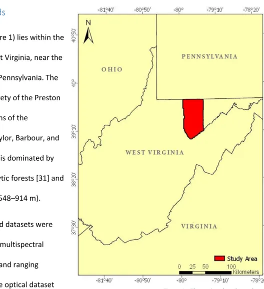
The study area (Figure 1) lies within the northeastern section of West Virginia, near the borders with Maryland and Pennsylvania. The study area includes the entirety of the Preston County, as well as proportions of the

neighboring Monongalia, Taylor, Barbour, and Tucker counties. This region is dominated by Appalachian mixed mesophytic forests [31] and the terrain is mountainous (548–914 m).

Two remotely sensed datasets were used in this analysis: optical multispectral imagery and light detection and ranging (LIDAR) point cloud data. The optical dataset comprises leaf-on National Agriculture Imagery

Program (NAIP) orthoimagery collected primarily during 17–30 July 2011. A very small portion of the NAIP imagery was collected on 10 October 2011. The NAIP imagery consists of four spectral bands (red (590–675 nm), green (500–650 nm), blue (400–580 nm), and near-infrared (NIR) (675–850 nm)), with an 8-bit radiometric resolution and a spatial resolution of 1 m [32]. The data were provided as

uncompressed digital orthophoto quarter quadrangles (DOQQs) in a .tiff format. The study area is covered by 108 individual DOQQ NAIP images, representing 260,975 ha or 4.2% of the total area of the state of West Virginia.

(25)

18

The LIDAR data were acquired using an Optech ALTM-3100C sensor through a series of aerial flights between 28 March and 28 April 2011. The LIDAR scanner had a 36° field of view and a frequency of 70,000 Hz. The LIDAR data were acquired at a flying height of 1,524 m above the ground with an average flight speed of 250 km/h. The flight lines of the LIDAR dataset had an average of 30% overlap. The LIDAR data include elevation, intensity, up to four returns, and a vendor-provided basic

classification of the points [33]. The LIDAR data were formatted as a .las version 1.2 point cloud. In total, 1164 LIDAR tiles containing a combined total of 5.6 x 109 points were used in the analysis. A preliminary investigation indicated that little change occurred during the approximately three to four-month temporal gap between the LIDAR and NAIP acquisitions.

Four land-cover classes were mapped: forest, grassland, water, and other. The forest class is primarily closed-canopy deciduous and mixed forests. The grassland class comprises areas dominated by non-woody vegetation. The water class includes both impoundments and natural waterbodies. The other class encompasses areas characterized by bare soil, exposed rock, impervious surfaces, and croplands.

(26)

19

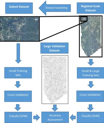
2.2. Experimental Design

Sample selection includes three components: sample size, sampling region, and sampling method. The sample size

specifies the number of training samples in the training set. The sampling region indicates whether samples are collected from the entire study area or only a limited sub region. The sampling method specifies the protocol for selecting samples, for example, random or deliberative.

In this study, four sampling methods are used to generate training data sets, which are then used with three

cross-validation methods in SVM classifications (Figure 2). The samples are selected from the entire study area or from only a small geographic subset of the study area, and in all cases, the classifier is applied to the entire regional-scale dataset. The error for all classifications is evaluated using a large independent validation dataset acquired from the entire regional-scale dataset.

(27)

20

2.3. Data Processing

A normalized-digital surface model (nDSM) and intensity rasters were generated as input variables for the classification from the LIDAR point cloud data. The LIDAR intensity raster was

generated using the first returns only and the LAS Dataset to Raster function in ArcMap 10.5.1 [34]. The LIDAR intensity data has proven to be beneficial for separating land-cover surfaces such as grassland, trees, buildings, and asphalt roads. [35–37]. The LIDAR intensity data was not normalized due to the limited LIDAR metadata which prevented the normalization for distance. Previous research indicates that LIDAR intensity information is still useful for land-cover classifications without this correction [38]. The nDSM was generated by subtracting a rasterized bare earth digital elevation model (DEM) from a digital surface model (DSM) produced from the ground and first returns, respectively. The LIDAR-derived surfaces were rasterized at 1 m, matching the pixel size of the NAIP orthoimagery. nDSMs have been demonstrated to be useful for characterizing the varying heights of natural and man-made objects in GEOBIA studies [39].

The 108 NAIP orthoimages were mosaicked into a single large NAIP image mosaic using the Mosaic Pro tool within ERDAS Imagine 2016. Color-balancing was used to reduce the radiometric variations between the NAIP images, since they were acquired from different flights and times [40]. The NAIP mosaic was clipped to the extent of the LIDAR rasters. The NAIP and LIDAR rasters were then combined to form a single layer stack with six bands: four NAIP (Red, Green, Blue, and NIR) and two LIDAR (nDSM and Intensity).

2.4. Image Segmentation

The Trimble eCognition Developer 9.3 multi-resolution segmentation (MRS) algorithm was used as the segmentation method [41]. MRS is a bottom-up region-growing segmentation approach. Equal weighting was given to all six input bands for the segmentation. Preliminary segmentation trials found that a large number of artefacts were created by the image segmentation, apparently due to the

(28)

21

“sawtooth” scanning pattern of the OPTECH ALTM 3100 sensor and the 1 m rasterization process [42]. A 5 x 5 pixel median filter was therefore applied to both the nDSM and Intensity rasters prior to

segmentation to reduce the problem.

MRS has three user-set parameters: scale, shape, and compactness [43]. The scale parameter (SP) is regarded as the most important of the three parameters as it controls the size of the image objects [44–46]. The Estimation of Scale Parameter (ESP2) tool developed by Drăguţ et al. [45] was used to estimate the optimal scale parameter for the segmentation. The ESP2 tool generates image-objects using incrementally increasing SP values and calculates the local variance (LV) for each scale. The rate of change of the local variance (ROC-LV) is then plotted against the SP. In theory, peaks in the ROC-LV curve indicate segmentation levels in which segments most accurately delineate real world objects and thus optimal SPs for the segmentation [45].

Due to the high processing and memory demands of the ESP2 tool, three randomly selected subset areas were chosen to apply the ESP2 process rather than attempting to run the tool across the entire regional-scale dataset. The three subset tests indicated optimal SP values of 97, 97, and 104. The intermediate value of 100 was therefore chosen for the segmentation of the entire image. Alterations of the shape and compactness parameters from their defaults of 0.1 and 0.5 respectively did not seem to improve the quality of the segmentation, and therefore these values were left unchanged. The

segmentation generated 474,614 image segments.

2.5. Dataset Subsetting

The subsetting tool in eCognition was used to extract the subset dataset from the regional dataset. The location of the subset was selected so that it included all four classes of interest. The total area of the subset dataset was approximately 4.19% of the area of the regional-scale dataset and comprised 21,777 image objects.

(29)

22

2.6. Segment Attributes Used for Classification

A total of 35 spectral and geometric attributes (Table 1) were generated for each image object (segment); these attributes were used as the predictor variables for the classification. Examples of the spectral attributes include the object’s means and standard deviations for each band and the geometric attributes include object asymmetry, compactness, and roundness. The object’s mean normalized difference vegetation index (NDVI) was also included as it is a commonly used spectral index used with NAIP data [47].

Table 1 - Spectral and geometric attributes of the segments

Attribute Type Attributes Number of Attributes

Spectral

Mean (Blue, Green, Intensity, NIR, Red, nDSM), Mode (Blue, Green, Intensity, NIR, Red, nDSM), Standard deviation (Blue, Green, Intensity, NIR, Red, nDSM), Skewness (Blue, Green, Intensity, NIR,

Red, nDSM), Brightness

25

Geometric Density, Roundness, Border length, Shape index, Area, Compactness,

Volume, Rectangular fit, Asymmetry 9

Spectral

Indices Mean NDVI 1

2.7. Sample Data Selection

As image-objects are the base unit of analysis in this study, an object-based sampling approach was used for the collection of the samples. Two spatial scales were employed: a small subset and a regional scale, encompassing the entire study area. A large regional sample (n = 10,000) from the regional-scale dataset was collected to provide a benchmark representing an assumed maximum accuracy possible with this dataset. Since the subset area is 4.19% of the regional scale data set, the sample size for the subset area was set to n = 419 samples (4.19% of 10,000). This sample set is termed the small subset dataset. In addition, a small regional sample (n = 419) was selected from the entire regional scale data set to provide a direct comparison with the small subset sample dataset. In summary, three categories of

(30)

23

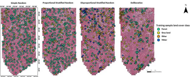
datasets were collected at two spatial scales and two sample sizes: samples from a small limited region within the study area (small subset sample) (Figure 3) and two sets of samples collected from across the study area, one encompassing a small number of samples (small regional sample) (Figure 4) and another encompassing a large number (large regional sample) (Figure 5).

For each of these three categories of spatial scales and sampling sizes, four sampling methods were employed: simple random, proportional stratified random, disproportional stratified random, and deliberative. All samples were manually labeled by the analyst. In total, 53,352 samples were collected for this analysis. The number of samples for each training and validation sample sets is summarized in Tables 2a–c.

Figure 3 - The subset area location and subset training samples overlaid on false color infrared composite of National Agricultural Imagery Program (NAIP) orthoimagery (Bands 4, 1, and 2 as RGB).

(31)

24

Figure 4 - The small regional training samples displayed over false color infrared composite of NAIP orthoimagery (Bands 4, 1, and 2 as RGB).

(32)

25

Table 2a- Small subset sample sets.

Number of samples per class

Sample Name Forest Grass Other Water

Total # of Samples Small Subset Simple Random 290 67 53 9 419 Small Subset Proportional Stratified Random 305 59 35 20 419 Small Subset Disproportional Stratified Random 209 84 84 42 419 Small Subset Deliberative 139 100 100 80 419

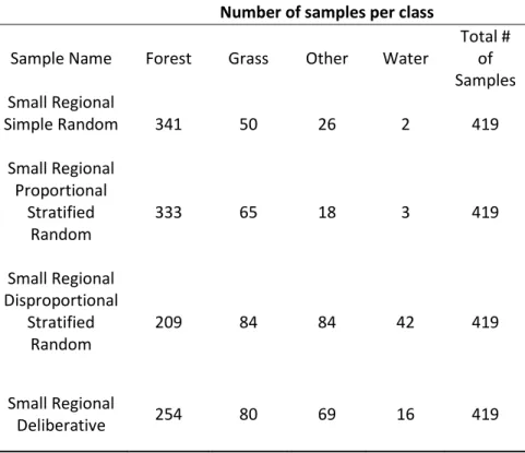
Table 2b. Small regional sample sets.

Total # of Samples Small Regional Simple Random 341 50 26 2 419 Small Regional Proportional Stratified Random 333 65 18 3 419 Small Regional Disproportional Stratified Random 209 84 84 42 419 Small Regional Deliberative 254 80 69 16 419

(33)

26

Table 2c. Small regional sample sets.

Total # of Samples Large Regional Simple Random 8183 1178 600 39 10000 Large Regional Proportional Stratified Random 7984 1553 408 55 10000 Large Regional Disproportional Stratified Random 5000 2000 2000 1000 10000 Large Regional Deliberative 6087 1897 1651 365 10000

2.7.1. Simple Random Sampling

The eCognition version 9.3 client does not offer a tool for selecting random samples, and therefore the select random polygon tool in QGIS was used.

(34)

27

2.7.2. Proportional Stratified Random Sampling

Because a stratified approach requires a priori strata, a rule-based classification developed through the expert system was applied to both the regional-scale dataset and the subset dataset (Figure 6) to estimate the strata sizes for the subset and regional datasets.

The ruleset contained 16 individual rules. The accuracy of the rule-based classifications was evaluated using the samples from the large regional-scale validation dataset and had an overall accuracy of 98.1%. The strata size for both the subset and regional-scale datasets were determined by the total area occupied by each class. Table 3 summarizes the proportions of the strata for both datasets. Simple random sampling was used within each stratum to obtain samples for both the subset and regional-scale datasets.

(35)

28

Table 3. Class strata sizes for subset and regional datasets.

2.7.3. Disproportional Stratified Random Sampling

It was not possible to test an equalized stratified sampling approach because the water class is too rare to provide sufficient samples for a 25% proportion. Consequently, a disproportional stratified approach was chosen. For this sample, the class proportions were defined as 50% forest, 20% grassland, 20% other, and 10% water. These proportions were selected as intermediate values between the random and equalized stratified proportions to ensure a larger representation of the less common classes than in the random dataset. The same values were used for the small subset and small and large regional sample sets.

2.7.4. Deliberative Sampling

The deliberative sample was produced via on-screen digitizing by the analyst using the sample selection tool in eCognition Developer. No attempt was made to avoid spatial autocorrelation in the samples selected, for example, by avoiding samples that were spatially adjacent, because manual selection of samples is generally characterized by autocorrelation [48].

2.8. Cross-Validation Strategies

The cross-validation tuning methods were conducted using the trainControl function within the caret package [49] in R Studio 1.1.383. A separate classification was conducted for each cross-validation tuning method used and each sample set. The three cross-validation strategies tested were k-fold, leave-one-out, and Monte Carlo.

Class Proportion of Total Area Occupied

Subset Dataset Regional Dataset

Forest 72.73% 79.84%

Grassland 14.10% 15.53%

Other 8.34% 4.08%

(36)

29

2.9. Supervised Classification

A radial basis function kernel (RBF) Support Vector Machines (SVM) was chosen as the supervised machine learning classifier for several reasons:

1. SVM is a commonly used supervised classifier in remote sensing analyses [17].

2. SVM is a non-parametric classifier, meaning it makes no assumption regarding the underlying data distribution. This may be advantageous for a small sample set [50].

3. SVMs are able to perform well with relatively small training datasets when compared to other commonly used classifiers.

4. SVMs are attractive for their ability to find a balance between accuracy and generalization [51]. A total of 36 individual classifications were conducted, each using a different combination of sample and validation methods: 3 categories of approaches at different spatial scales and sample sizes (small subset, small regional, and large regional) x 4 sample selection methods (simple random, proportional stratified random, disproportional stratified random, and deliberative) x 3 cross-validation tuning methods (k-fold, leave-one-out, and Monte Carlo) = 36 classifications.

Table 4 details all subset-trained and regional-trained classifications. The SVM classifications were conducted within R Studio client version 1.1.383 using the e1071 [52] and caret packages [49] on a Dell Optiplex 980 workstation with an Intel i7 2.80 GHz processor with 16.0 GB of memory running Windows 8.1 Enterprise. The processing time for all classifications were recorded using the microbenchmark package [53]. Processing runtime values should be interpreted as indications of relative speed and not as absolute values as they are highly dependent on the system architecture, CPU allocation, memory availability, and background system processes, among other factors.

(37)

30

Table 4. Classifications and associated abbreviations based on the sample selection method, training sample size, region of area collected, and cross-validation method.

Cross-Validation Method k-Fold (KF) Monte Carlo (MC) Leave- One-Out (LOO) k-Fold (KF) Monte Carlo (MC) Leave- One-Out (LOO) k-Fold (KF) Monte Carlo (MC) Leave- One-Out (LOO) Small Subset-Trained Classification

Small Regional-Scale Trained Classification

Large Regional-Scale Trained Classification Sample Selection Method Simple Random (SR) Small- Subset-(SR-KF) Small- Subset-(SR-MC) Small- Subset-(SR-LOO) Small- Regional-(SR-KF) Small- Regional-(SR-MC) Small- Regional-(SR-LOO) Large- Regional-(SR-KF) Large- Regional-(SR-MC) Large- Regional-(SR-LOO) Proportional Stratified Random (PSTR) Small- Subset-(PSTR-KF) Small- Subset-(PSTR-MC) Small- Subset- (PSTR-LOO) Small- Regional-(PSTR-KF) Small- Regional- (PSTR-MC) Small- Regional- (PSTR-LOO) Large- Regional-(PSTR-KF) Large- Regional- (PSTR-MC) Large- Regional- (PSTR-LOO) Disproportional Stratified Random (DSTR) Small- Subset-(DSTR-KF) Small- Subset-(DSTR-MC) Small- Subset- (DSTR-LOO) Small- Regional-(DSTR-KF) Small- Regional- (DSTR-MC) Small- Regional- (DSTR-LOO) Large- Regional-(DSTR-KF) Large- Regional- (DSTR-MC) Large- Regional- (DSTR-LOO) Deliberative (DL) Small- Subset-(DL-KF) Small- Subset-(DL-MC) Small- Subset-(DL-LOO) Small- Regional-(DL-KF) Small- Regional-(DL-MC) Small- Regional-(DL-LOO) Large- Regional-(DL-KF) Large- Regional-(DL-MC) Large- Regional-(DL-LOO)

2.10. Error Assessment

Each of the trained classifications was tested against a large, randomly sampled validation dataset (n = 10,000) collected from the regional-scale dataset. Results for each classification were reported in a confusion matrix programmed via the caret package in the R statistical client. User’s and producer’s accuracies were calculated as well as overall accuracy and the kappa coefficient. Additionally, McNemar’s test [54] was used to evaluate the statistical significance of differences observed between the k-fold tuned classifications. McNemar’s test is a non-parametric evaluation of the statistical differences between two classifications with related samples [55]. A p-value smaller than 0.05 indicates a one-sided 95% confidence that the differences in accuracy between the classifications are statistically significant.

(38)

31

3. Results and Discussion

3.1. Performance of Sample Selection Methods

Figure 7 summarizes the overall accuracies of the classification of the entire regional dataset using the various training samples and k-fold (k = 10) cross-validation. Within each spatial scale and sample size (i.e., subset, small regional, and large regional), the disproportional stratified random (DSTR) samples consistently resulted in the highest overall accuracy although it is notable that variations between the performance of the classifications trained using the different statistical-based sampling methods were small, less than 2%.

Figure 7 - Overall accuracies of the regional classifications using small subset, small regional, and large regional training datasets and k-fold (k=10) cross-validation tuning.

Despite the small differences between some of the classification accuracies, the McNemar’s test results, shown in Table 5, indicate that most of the differences were statistically significant. The only

(39)

32

exceptions were the differences in the classification accuracies for the large regional-trained SR, PSTR, and DSTR, which indicates that when the sample size is very large (n = 10,000 in this case), differences between sampling methods is less important.

Classifications trained with the SR sample resulted in a slightly lower accuracy than those trained with the PSTR and DSTR samples. This suggests that sample stratification is advantageous for SVM classifiers, as stratification ensures that rare classes are sampled at a rate that is either equal to or greater than their proportion in the dataset, depending on whether proportional or disproportional stratified approaches are selected.

The DSTR sampling method was designed to provide a much larger number of samples from minority classes, such as the water and other classes, than the simple random or proportional stratified random sampling methods (Table 2a–c). Using SR sampling, the number of samples from the minority classes may vary greatly, depending on random chance, especially when the total number of samples is small (e.g., 419 in this case). This can be seen in the small-regional SR and PSTR sample sets, where only 2 and 3 samples, respectively, were collected for water (Table 2b). The number of samples selected for the rare classes is important; Waske et al. [56] found that SVM was negatively affected by dataset imbalance. Stehman [57] also found that sample stratification resulted in improved classification accuracy due to an increased sample selection from the minority classes. The results of our study emphasize the value of disproportional stratified sample selection to reduce class imbalance and ensure minority class representation in the training set.

(40)

33

Table 5. McNemar's test p-values for small subset, small regional, and large regional-trained classifications using k-fold (k=10) cross-validation tuning. (*Indicates the differences between classifications that are statistically significant, p < 0.05.)

The classifications trained from the deliberative (DL) samples consistently had lower accuracies across all sample sets (Figure 7). The low accuracy for the classifications with the DL samples indicates that samples acquired though expert selection of the training data did not adequately characterize the dataset. Notably, the DL samples have higher spatial autocorrelation than samples collected via the statistical-based methods (Figure 5). This is not surprising; as noted previously, human-based

Subset-SR-KF Subset- PSTR-KF Subset- DSTR-KF Subset-DL-KF Small- Regional-SR-KF Small- Regional-PSTR-KF Small- Regional-DSTR-KF Small- Regional-DL-KF Large- Regional-SR-KF Large- Regional-PSTR-KF Large- Regional-DSTR-KF Large- Regional-DL-KF <0.001* <0.001* <0.001* <0.001* <0.001* <0.001* <0.001* <0.001* <0.001* <0.001* <0.001* Subset-SR-KF 0.007* <0.001* <0.001* <0.001* 0.004* <0.001* <0.001* <0.001* <0.001* <0.001* Subset-PSTR-KF <0.001* 0.043* <0.001* <0.001* <0.001* <0.001* <0.001* <0.001* <0.001* Subset-DSTR-KF <0.001* <0.001* <0.001* 0.009* <0.001* <0.001* <0.001* <0.001* Subset-DL-KF 0.013* 0.002* <0.001* <0.001* <0.001* <0.001* <0.001* Small- Regional-SR-KF 0.031* <0.001* <0.001* <0.001* <0.001* <0.001* Small- Regional-PSTR-KF <0.001* <0.001* <0.001* <0.001* <0.001* Small- Regional-DSTR-KF <0.001* <0.001* <0.001* <0.001* Small- Regional-DL-KF 0.108 0.113 <0.001* Large- Regional-SR-KF 0.162 <0.001* Large- Regional-PSTR-KF <0.001* Large- Regional-DSTR-KF Large- Regional-DL-KF

(41)

34

deliberative sampling has a high potential for spatial autocorrelation [48]. High spatial autocorrelation in sample sets may result in a reduction in the effective sample size [13]. A univariate Moran’s I test indicates that the small subset, small regional, and large regional DL samples all show positive spatial autocorrelation, with values of 0.950, 0.692, and 0.985, respectively. While the SR, PSTR, and DSTR samples also contained positive spatial autocorrelation, ranging from 0.208 (subset-SR) to 0.661 (large-regional-DSTR), they showed less positive spatial autocorrelation than all DL sample sets. Stratified sampling, especially disproportional stratified sampling, tends to favor some autocorrelation, since samples are, by definition, not completely random.

The similar performance between the classifications trained from the small subset and small regional-scale samples and the much higher accuracy reported from the large regional-scale sample indicate that the geographic location of the sample may not be as important as the sample size in determining the accuracy of the supervised SVM classifications. This is notable as selecting a small sample from a subset area is less expensive in terms of effort than selecting a small sample from a regional-scale area, especially if field data collection is needed. It should also be mentioned that the regional-scale area in this analysis was generally homogenous, which allowed the selection of a single subset area that contained many examples of all four classes of interest. In areas or datasets that are more heterogeneous or contain extreme minority classes limited to separate geographic regions of a regional-scale dataset, multiple subset areas may be needed for subset-based sampling to be effective. The fact that the classifications trained from both small sample sets were less accurate than the large regional-trained benchmark classification emphasizes that large numbers of statistical-based samples can raise the accuracy of SVM classifications substantially.

3.2. Performance of Cross-Validation Tuning Methods

There was no consistent pattern for the overall accuracy of the classifications trained from the small subset samples and tuned using the three cross-validation methods (k-fold, Monte Carlo, and

(42)

35

leave-one-out). As seen in Figure 8a, when the SR samples were used as training data, the k-fold (KF) method provided slightly higher accuracy than the Monte Carlo (MC) or leave-one-out (LOO) cross-validation. MC proved the best method for the PSTR samples. KF, MC, and LOO tuning resulted in equal overall accuracies for the DSTR samples. Overall, the differences in overall accuracy between the tuning methods on the small subset statistical-sample trained classifications was less than 1%.

The cross-validation tuning methods using the small regional SR, PSTR, and DSTR training data applied to the SVM classification all showed high values for overall accuracy (Figure 8b) and inconsistent results for the different tuning methods, similar to the results of the small subset training data. LOO had slightly lower performance on the SR classifications, but this decrease in performance was also less than 1%. The DSTR classifications had the highest overall accuracy, irrespective of the cross-validation tuning methods, with the MC- and LOO-tuned DSTR classifications resulting in 94.8% and the k-fold tuned-DSTR resulting in 94.7% overall accuracy.

For the large-regional statistical sample-trained classifications, the MC- and KF-tuned

classifications consistently outperformed LOO. This indicates that LOO is less effective for tuning than KF and MC when dealing with large statistical-based sample sets. Both MC and KF had the same overall accuracy for the large-regional SR, PSTR, and DSTR classifications.

The deliberative-trained classifications for both the small subset and regional scales had much lower performances than the statistical based classifications. For the small-regional DL classifications, LOO matched the overall accuracy of KF and MC at 89.6% (Figure 8b). However, for both the small-subset (Figure 8a) and large-regional DL classifications (Figure 8c), LOO tuning improved overall accuracy by 3.6% and 1.2%, respectively over the KF-DL classifications.

The confusion matrices of the small subset-DL-KF (Table 6), MC (Table 7), and LOO (Table 8) show that the increase in performance of the small subset-DL-LOO classification was due to a substantial