Software fault prediction using object-oriented metrics

(1)

Software Fault Prediction

using

Object-Oriented Metrics

Lov Kumar

Department of Computer Science and Engineering

National Institute of Technology Rourkela

Rourkela-769008, Odisha, India

June 2014

(2)

Software Fault Prediction

using

Object-Oriented Metrics

Thesis submitted in partial fulfillment of the requirements for the degree of

Master of Technology

in

Computer Science and Engineering

(Specialization: Software Engineering) by

Lov Kumar

(Roll No.- 212CS3371)

under the supervision of

Prof. S. K. Rath

Department of Computer Science and Engineering

National Institute of Technology Rourkela

Rourkela, Odisha, 769 008, India

(3)

Department of Computer Science and Engineering

National Institute of Technology Rourkela

Rourkela-769 008, Odisha, India.

Certificate

This is to certify that the work in the thesis entitledSoftware Fault Prediction using Object-Oriented Metrics by Lov Kumar is a record of an original research work carried out by him under my supervision and guidance in partial fulfillment of the requirements for the award of the degree of Master of Technology with the specialization of Software Engineering in the department of Computer Science and Engineering, National Institute of Technology Rourkela. Neither this thesis nor any part of it has been submitted for any degree or academic award elsewhere.

Place: NIT Rourkela (Prof. Santanu Ku. Rath)

Date: June 1, 2014 Professor, CSE Department NIT Rourkela, Odisha

(4)

Acknowledgment

I am grateful to numerous local and global peers who have contributed towards shaping this thesis. At the outset, I would like to express my sincere thanks to Prof. Santanu Ku. Rath for his advice during my thesis work. As my supervisor, he has constantly encouraged me to remain focused on achieving my goal. His observations and comments helped me to establish the overall direction to the research and to move forward with investigation in depth. He has helped me greatly and been a source of knowledge.

I am very much indebted to Prof. Santanu Ku. Rath, for his continuous encouragement and support. He is always ready to help with a smile. I am also thankful to all the professors at the department for their support.

I would like to thank all my friends and lab-mates for their encouragement and understanding. Their help can never be penned with words.

I must acknowledge the academic resources that I have got from NIT Rourkela. I would like to thank administrative and technical staff members of the Department who have been kind enough to advise and help in their respective roles.

Last, but not the least, I would like to dedicate this thesis to my family, for their love, patience, and understanding.

Lov kumar Roll-212cs3371

(5)

Abstract

Fault-prediction techniques aim to predict the fault prone software modules in order to streamline the effort to be applied in the later phases of software de-velopment. Many fault-prediction techniques have been proposed and evaluated for their performance using various performance criteria. However, due to the lack of compiling their performances in proper perspective, one significant issue about the viability of these techniques has not been adequately addressed. In this study, an adaptive cost evaluation framework is proposed that incorporates cost drivers for various fault removal phases, and performs a cost-benefit analysis for the misclassification of faults. Accordingly, our study focuses on investigat-ing two important and related research questions regardinvestigat-ing the viability of fault prediction. First, for a given software product, whether performing fault predic-tion analysis is economically effective or not?. In case of an positive affirmapredic-tion, then emphasis is provided on how to choose a fault prediction technique for an overall improved performance in terms of cost-effectiveness. In this study, Object-Oriented software metrics have been considered to provide requisite input data to design a classifier using statistical, machine learning and hybrid methods of soft computing. This work, also extends the study on finding the effectiveness of feature reduction techniques. From the obtained results, it is observed that performing fault prediction is quite desirable for those software systems, when the percentage of faulty modules are below the range of certain threshold value.

Keywords: ANN, ANGA, CSA, GA, linear regression, logistics regression, MNPSO, NGA, NCSA, NPSO, Naive Bayes, polynomial regression, PCA, PSO, SVM, RSA, Software fault estimation, software metrics.

(6)

List of Figures

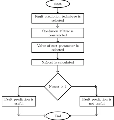
2.1 Decision chart representation to evaluate the estimated NEcost . . . 21

3.1 Artificial neural network . . . 30

3.2 Mean square error Vs No. of iteration . . . 35

3.3 Mean square error Vs No. of iteration . . . 35

4.1 Flow chart representing Neuro-GA execution . . . 43

4.2 Flow chart representing Neuro-PSO execution . . . 45

4.3 Flow chart representing Neuro-CSA execution . . . 47

4.4 Generation No. vs number of chromose having same fitness value . 49 4.5 Generation No. vs fitness value . . . 51

4.6 Generation No. vs fitness value . . . 53

(10)

List of Tables

1.1 Summary of literature on reliability prediction using software Metrics suite 4

1.2 Fault prediction effectiveness based on Cost evaluation model . . . 5

1.3 Software metrics . . . 6

1.4 Confusion matrix to classify a class as faulty and not-faulty . . . 7

2.1 Distribution of bugs in AIP version 1.6 . . . 14

2.2 Removal costs of test techniques (in staff hour per defects) . . . 19

2.3 Fault identification efficiencies of different test phase . . . 19

2.4 After applying Linear Regression . . . 22

2.5 After applying Polynomial Regression . . . 22

2.6 After applying Logistic Regression . . . 23

2.7 After applying Naive Bayes . . . 23

2.8 After applying SVM . . . 23

2.9 Result of experiment for Eclipse JDT Core . . . 23

3.1 Descriptive Statistics of Classes . . . 28

3.2 Correlations between the Metrics of Basili et al (lower) and Ellipse JDT core (upper) 29 3.3 Before applying ANN . . . 34

3.4 After applying ANN . . . 34

3.5 After applying ANN . . . 35

3.6 Fault removal cost for Eclipse JDT core . . . 37

4.1 Before applying regression . . . 49

4.2 After applying Neuro-GA . . . 50

(11)

LIST OF TABLES LIST OF TABLES

4.4 After applying Neuro-PSO . . . 52

4.5 After applying Modified Neuro-PSO . . . 52

4.6 After applying Neuro-CSA . . . 53

4.7 Fault removal cost for Eclipse JDT core . . . 54

(12)

LIST OF TABLES LIST OF TABLES

List Of Abbreviation

ANN Artificial neural network

DIT Depth of inheritance tree

CBO Coupling between objects

CSA Clonal Selection Algorithm

Ecost Estimate fault removal cost with using fault prediction

FP False Positive

FN False Negative

GA Genetics algorithm

LCOM Lack of cohesion among methods

N Ecost Normalized Estimated fault removal cost

NOA Number of attributes

NOAI Number of attributes inherited

NOC Number of children

NLOC Number of line of codes

NOM Number of methods

NOMI Number of methods inherited

NOPA Number of private attribute

NP¯OA Number of public attribute

NOPM Number of private methods

NP¯OM Number of public methods

PCA Principal components analysis

PSO Particle Swarm Optimization

RSA Rough set analysis

RFC Response for class

SVM Support Vector Machine

TP True Positive

TN True Negative

Tcost Estimate fault removal cost with using testing

(13)

Introduction

Literature Review Software metrics Performance Parameter Motivation Thesis Organization

(14)

Chapter 1 Introduction

Fault prediction is necessary in software development life cycle in order to reduce the probable software failure and is carried out mostly during initial planning to identify fault-prone modules. Fault prediction not only gives an insight to the need for increased quality of monitoring during software development but also provides necessary tips to undertake suitable verification and validation approaches that eventually lead to improvement of efficiency and effectiveness of fault prediction. Effectiveness of a fault prediction is studied by applying a part of previously known data related to faults and predicting its performance against other part of the fault data. Several researchers have worked on building prediction models for software fault prediction but less emphasis has been given on the study of effectiveness of fault prediction.

Present day software development is mostly desired to be based on Object-Oriented (OO) paradigm. The quality of OO software can be best assessed by the use of software metrics. A number of metrics have been proposed by researchers and practitioners to evaluate the quality of software. Some of the software metrics available in literature are as follows: Abreu MOOD metric suite [1], Bansiya and Davis (QMOOD metrics suite) [2], Bieman and Kang [3], Briand et al. [4], Etzkornet al. [5], Halstead [6], Henderson-sellers [7], Li and Henry [8], McCabe [9], Tegarden et al. [10], Lorenz and Kidd [11] and CK metric [12] suite.

These metrics help to verify the quality attributes of a software such as effort and fault proneness. The usefulness of these metrics lies in their ability to predict

(15)

1.1 Literature Review Introduction

to FURPS model such as functionality, usability, reliability, Portability and sup-portability. This study mostly focus on the aspect of improving reliability of a software by reducing the number of faults in the software.

In order to estimate the reliability of a class, several traditional methods are available in literature. But less importance has been given on using machine learning techniques. Artificial intelligence techniques, a subset of machine learn-ing methods have the ability of computer, software and firmware to measure the properties of a class, that human beings recognize as intelligent behavior. These methods are able to approximate the non-linear function with more precision. Hence they can be applied for quality estimation in order to achieve better accu-racy.

1.1 Literature Review

This section presents a review of literature on the application of software metrics. Table 1.1 shows the summary of Empirical Literature on software metrics.

Basiliet al.,[13] experimentally analyzed the impact of CK metric suite in fault prediction. Briandet al.,[14] found out the relationship between fault and the met-rics using univariate and multivariate logistic regression models. Tang et al., [16] investigated the dependency between CK metric suite and the Object-Oriented system faults. Emam et al., [18] conducted empirical validation on Java applica-tion and found that export coupling has great influence with faults. Khoshgoftaar

et al., [21], Hochman [22] conducted experimental analysis on telecommunication model and found that artificial neural network (ANN) model is give accurately output than other discriminant model. In their approaches, nine software metrics were used for modules developed in procedural paradigm. Since then, ANN mod-els have taken a rise in their usage for prediction modeling. Hence, in this study, different ANN models are used for fault prediction of embedded software.

Also few researchers have presented cost based evaluation models for predicting the effectiveness of fault prediction. In this section, the study related to the measure of cost effectiveness for fault prediction has been tabulated in Table 1.2.

(16)

1.1 Literature Review Introduction

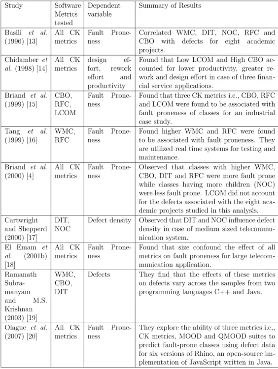
Table 1.1: Summary of literature on reliability prediction using software Metrics suite Study Software Metrics tested Dependent variable Summary of Results Basili et al. (1996) [13] All CK metrics Fault Prone-ness

Correlated WMC, DIT, NOC, RFC and CBO with defects for eight academic projects. Chidamber et al. (1998) [14] All CK metrics design ef-fort, rework effort and productivity

Found that Low LCOM and High CBO ac-counted for lower productivity, greater re-work and design effort in case of three finan-cial service applications.

Briand et al. (1999) [15] CBO, RFC, LCOM Fault Prone-ness

Found that three CK metrics i.e., CBO, RFC and LCOM were found to be associated with fault proneness of classes for an industrial case study. Tang et al. (1999) [16] WMC, RFC Fault Prone-ness

Found higher WMC and RFC were found to be associated with fault proneness. They are utilized real time systems for testing and maintenance. Briand et al. (2000) [4] All CK metrics Fault Prone-ness

Observed that classes with higher WMC, CBO, DIT and RFC were more fault prone while classes having more children (NOC) were less fault prone. LCOM did not account for the defects associated with the eight aca-demic projects studied in this analysis. Cartwright

and Shepperd (2000) [17]

DIT, NOC

Defect density Observed that DIT and NOC influence defect density in case of medium sized telecommu-nication system. El Emam et al. (2001b) [18] All CK metrics Fault Prone-ness

Found that size confound the effect of all metrics on fault proneness for large telecom-munication application. Ramanath Subra-manyam and M.S. Krishnan (2003) [19] WMC, CBO, DIT

Defects They find that the effects of these metrics on defects vary across the samples from two programming languages C++ and Java.

Olague et al. (2007) [20] All CK metrics Fault Prone-ness

They explore the ability of three metrics i.e., CK metrics, MOOD and QMOOD suites to predict fault-prone classes using defect data for six versions of Rhino, an open-source im-plementation of JavaScript written in Java.

(17)

1.2 Software Metrics Introduction

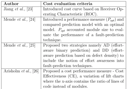
Table 1.2: Fault prediction effectiveness based on Cost evaluation model

Author Cost evaluation criteria

Jiang et al., [23] Introduced cost curve based on Receiver Op-erating Characteristic (ROC).

Mende et al., [24] Introduced a performance measure (Popt) and

compared prediction model with an optimal model. Popt accounted module size to

eval-uate the performance of a fault-prediction technique.

Mende et al., [25] Proposed two strategies namely AD aware binary prediction) and DD (effort-aware prediction based on defect density) to include the notion of effort awareness into fault-prediction techniques.

Arisholmet al.,[26] Proposed a cost performance measure - Cost Effectiveness (CE), a variation of lift charts where the x-axis contains the ratio of lines of code instead of modules.

In this study, linear regression, polynomial regression, logistic regression, Naive Bayes and SVM models have been considered so as to predict software quality by classifying a class as faulty or not faulty .

In literature, classification models are mostly built using statistical analysis. Neural networks (NN) have seen an explosion of interest over the years, and are being successfully applied across a range of problem domains. When the problems of classification, prediction, NN are being used, NN can be used as a technique to design prediction model because it is a very sophisticated modeling technique that enables modeling of complex function. In this thesis work, software metrics has been considered for quality estimation using various statistical and artificial intelligence techniques.

1.2 Software Metrics

A software metric is the measurement of a individual characteristic of a program’s efficiency or performance and also used to measures the attributes of software prod-ucts and processes. At present, software development based on Object-Oriented (OO) Paradigm is becoming more and more pronounced. The Object-Oriented

(18)

1.2 Software Metrics Introduction

paradigm for the software development differs from traditional procedural so the traditional metrics can not be applied on OO software.

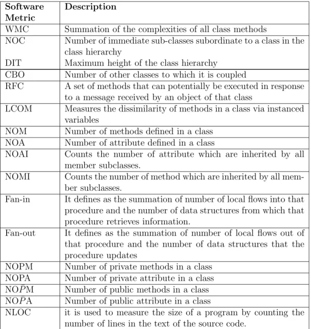
A number of OO software metrics have been proposed by researchers and practitioners to evaluate the quality of OO software. The most commonly used metric suites are: Abreu MOOD metric suite [1], Bansiya and Davis (QMOOD metrics suite) [2], Bieman and Kang [3], Briand et al. [4], Etzkorn et al. [5], Halstead [6], Henderson-sellers [7], Li and Henry [8], McCabe [9], Tegarden et al. [10], Lorenz and Kidd [11] and CK metric [12] suite. Table 1.3 gives the basic definitions of software metric.

Table 1.3: Software metrics

Software Metric

Description

WMC Summation of the complexities of all class methods

NOC Number of immediate sub-classes subordinate to a class in the class hierarchy

DIT Maximum height of the class hierarchy

CBO Number of other classes to which it is coupled

RFC A set of methods that can potentially be executed in response to a message received by an object of that class

LCOM Measures the dissimilarity of methods in a class via instanced variables

NOM Number of methods defined in a class NOA Number of attribute defined in a class

NOAI Counts the number of attribute which are inherited by all member subclasses.

NOMI Counts the number of method which are inherited by all mem-ber subclasses.

Fan-in It defines as the summation of number of local flows into that procedure and the number of data structures from which that procedure retrieves information.

Fan-out It defines as the summation of number of local flows out of that procedure and the number of data structures that the procedure updates

NOPM Number of private methods in a class NOPA Number of private attribute in a class NO ¯PM Number of public methods in a class NO ¯PA Number of public attribute in a class

NLOC it is used to measure the size of a program by counting the number of lines in the text of the source code.

(19)

1.3 Performance evaluation parameters Introduction

1.3 Performance evaluation parameters

The following sub-sections give the basic definitions of the performance parameters used for fault prediction.

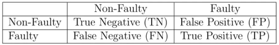
Table 1.4: Confusion matrix to classify a class as faulty and not-faulty Non-Faulty Faulty

Non-Faulty True Negative (TN) False Positive (FP) Faulty False Negative (FN) True Positive (TP) The confusion matrix are categories into four category :

i. True positives (TP) are the number of modules correctly classified as faulty modules.

ii. False positives (FP) refer to not-faulty classes incorrectly labeled as faulty classes.

iii. True negatives (TN) correspond to not-faulty modules correctly classified as such.

iv. Finally, false negatives (FN) refer to faulty classes incorrectly classified as not-faulty classes.

These are the performance parameter used to measures the classification tech-niques.

Precision

It is used to measure the degree to which the repeated measurements under unchanged conditions show the same results.

P recision= T P

F P +T P (1.1)

Recall

Recall indicates the how many of the relevant item that are to be identified. it is represented as:

Recall = T P

F N +T P (1.2)

(20)

1.4 Motivation Introduction

F-Measure

F-Measure combine the precision and recall numeric value to give a single score, which is defined as the harmonic mean of the recall and precision. F-Measure is expressed as:

F −M easure= 2∗Recall∗P recision

Recall+P recision (1.3)

Specificity

Specificity focus on how effectively a classifier identifies the negative labels. It is defined as:

Specif icity = T N

F P +T N (1.4)

Accuracy

Accuracy measure is the proportion of predicted fault prone modules that are inspected out of all modules. It is defined as:

Accuracy = T N +T P

T P +T N +F P +F N (1.5)

1.4 Motivation

The majority of software bugs are small in nature, which cause large inconvenience that can be worked around by the user. Some noticeable cases wherein a simple mistake can affect millions and even cause injury and leads to loss of life. Software code, written by humans has a probability that every piece of software has fault or undocumented features. That is, the software does not meet the requirements. These faults can be due to bad design, problem misunderstanding, or just simple error just like a typo in a book. Unlike a book is read by a human who can usually infer the meaning of a misspelled word, the software is read by computers, which are comparatively stupid, and will perform what they are instructed to do. There are some major computer system failures caused by software bugs, such as:

(21)

1.4 Motivation Introduction

Nearly five patient deaths in the 1980’s due to bugs in “Therac-25 radiation

therapy” machine.

In 1994, nine passengers are died in helicopter crashed in Chinook (Scotland)

due to systems error in helicopter.

In mar 2002, Britain’s National Tax system overcharges 100,000 erroneous

due to fault in their software system.

In Japan’s largest banks going off line for 24 hr, Internet banking services

(IBS) being shut down for three days, delays in salary payments worth $1.5

billion into the accounts of 620,000 people and a backlog of more than 1 million unprocessed payments worth around $9 billion.

In 2011, twenty two people wrongly arrested in Australia due to fault in new

zealand $54.5 million courts computer system.

In Apr 1992, first F-22 Raptor was crashed while landing at Edwards Air

Force Base due to fault in flight controlling software system.

In 2004, A2LL software which handling social services and unemployment

in Germany transfer a payments to invalid account number due to failure in their system.

Thus, reducing these type of failure, Software fault prediction is one of the different strategies, which are conducted during the very beginning of software development life cycle. Fault prediction information not only for the increasing quality of software during the development but also give an information to un-derstand suitable validation and verification activities in order to improve the effectiveness.

(22)

1.5 Thesis Organization Introduction

1.5 Thesis Organization

The rest of thesis is organized as follow:

In Chapter-2, cost evaluation framework has been proposed which performs

cost based analysis for misclassification of faults. This Chapter also focuses on investigating two important and related research questions regarding the viability of fault prediction. First, for a given software product, whether performing fault prediction analysis is economically effective or not?. In case of an positive affirmation, then emphasis is provided on how to choose a fault prediction technique for an overall improved performance in terms of cost-effectiveness

In Chapter-3, artificial neural network (ANN), has been used to design a

classifier, to classify a class as faulty and not faulty. In this chapter a case study of Eclipse JDT core has been considered for predicting the fault prone-ness.

In Chapter-4, hybrid approach of artificial neural network and optimization

algorithms i.e., genetics algorithm (GA), clonal selection algorithm (CSA) and Particle Swarm Optimization (PSO) have been used to design a classifier to classifying a class as faulty and not faulty. Here also same case study of Eclipse JDT core has been considered for predicting the fault proneness.

(23)

Effectiveness of fault prediction Techniques

Introduction Research Background Proposed work Cost analysis model Summary

(24)

Chapter 2 Effectiveness of fault prediction

Techniques

2.1 Introduction

Software fault prediction is helpful in deciding the amount of effort needed for soft-ware development. In literature it is observed that, a good number of approaches have been studied and evaluated on software products to determine best suitable approach for fault prediction based on certain performance criteria (precision, re-call, accuracy etc.). However very less significant work has been done on feasibility of fault prediction approach. In this study, a cost evaluation framework has been proposed which performs cost based analysis for misclassification of faults. Ac-cordingly, this study focuses on investigating two important and related research questions regarding the viability of fault prediction. First, for a given project, do the developer feel that the fault prediction results useful? In case of an affirmative answer, then it is desirable to investigate as to how to choose a fault prediction technique for an overall improved performance in terms of cost effectiveness. The proposed framework is used to investigate the usefulness of various fault-prediction techniques. The investigation consisted of performance evaluation of five major fault-prediction techniques i.e, liner regression, polynomial regression, logistics re-gression, Naive Bayes and SVM on Eclipse JDT core. From the obtained results, it is observed that application of fault prediction models are useful for the projects with percentage of faulty modules less than a certain threshold.

(25)

2.2 RESEARCH BACKGROUND Effectiveness of fault prediction Techniques

2.2 RESEARCH BACKGROUND

The following sub-sections highlight on the data set being used for fault predic-tion. Data was normalized to obtain better accuracy and then dependent and independent variables are chosen for fault prediction.

2.2.1 Empirical data collection

Metric suites are used and defined for different goals such as fault prediction, effort estimation, re-usability and maintenance. In this study, the mostly commonly used CK metric suite [27] is used for fault prediction. The metric values of the suite were extracted using Chidamber and Kemerer Java Metrics tool (CKJM). CKJM tools extracts OO metrics by processing the byte code of compiled Java classes. In this study, NASA and PROMISE [28] datasets are used to evaluate the impact of fault-prediction techniques over the fault removal cost using proposed model (NEcost).

2.2.2 Dependent and independent variables

The goal of this study is to establish the relationship between Object-Oriented metrics and fault proneness at the class level. In this study, a fault is used as a dependent variable and each of the CK metric is an independent variable. It is intended to develop a function between fault of a class and CK metrics suite (WMC, NOC, DIT, RFC, CBO, LCOM). Fault is a function of WMC, NOC, DIT, RFC, CBO and LCOM and can be represented as shown in the following equation:

F aults=f(W M C, N OC, DIT, CBO, RF C, LCOM) (2.1)

2.2.3 Case study

In this study, to analyze the effectiveness of the proposed approach, Ellipse JDT core was used as a case study.

(26)

2.3 Proposed work for fault predictionEffectiveness of fault prediction Techniques

2.2.4 Fault Data

To perform statistical analysis, bugs were collected from Promise data repository [28]. Table 2.1 shows the distribution of bugs based on the number of occurrence (in terms of percentage of class containing number of bugs) for Ellipse JDT core.

Table 2.1: Distribution of bugs in AIP version 1.6 No. of

Classes

% of bugs Number of as-sociated bugs 791 79.33 0 138 13.84 1 31 3.10 2 15 1.50 3 8 0.80 4 2 0.20 5 4 0.40 6 3 0.30 7 3 0.30 8 2 0.20 9 997 100.00

Ellipse JDT core contains 997number of different classes in which 79.33% of classes contain zero bugs i.e., out of 997 classes: 791 classes contains zero bugs, 13.84% of classes contain at least one bug, 3.10% of classes contain a minimum of two bugs, 1.50% of classes contain three bugs, 0.80% classes contain four bugs, 0.20% of classes contain five and nine bugs, 0.40% classes contain six bugs, 0.30% of classes contain seven and eight bugs.

2.3 Proposed work for fault prediction

The following sub-sections highlight on the various methods used for fault classi-fication.

2.3.1 Linear Regression models

Linear regression is the commonly used statistical technique [29]. It is used to find the linear (i.e., straight-line) relationship between variables.

(27)

The Univariate linear regression is represented as:

Y =β1X+β0 (2.2)

where Y represent the dependent variable and X represent the independent vari-able. β0, β1 are the constant and coefficient values respectively.

In case of multivariate linear regression, the linear regression is represented as:

Y =β0+β1X1+β2X2+...+βpXp (2.3)

WhereXi represent the independent variable and Y represent the dependent

vari-able, β0, βi are the constant and coefficient values respectively.

2.3.2 Polynomial regression models

Polynomial regression is the commonly used statistical technique. Polynomial models are useful in situations where the analyst knows that curvilinear effects are present in the true response function [29]. Polynomial models are also use-ful as approximating functions to unknown and possible very complex nonlinear relationship.

The Univariate Polynomial regression analysis is represented as:

Y =β0+β1X+β2X2+...+βnXn (2.4)

where Y is dependent variable, X is independent variable and β0, β1...βn are

the constant and coefficient values respectively.

Equation 2.4 shows the Univariate Polynomial regression model for nth order polynomial. In this report, second order polynomial is considered for finding the relationship between fault and CK metrics of the class. The second order polynomial is represented as:

Y =β0+β1X+β2X2 (2.5)

In case of multivariate second order Polynomial regression analysis, the Poly-nomial regression of two variables is based on:

Y =β0+β1X1+β2X2+β11X12+β22X22+β12X1X2 (2.6)

(28)

2.3.3 Logistic regression model

Logistic regression is the commonly used statistical technique. Which is a kind of regression analysis used for predicting the outcome of dependent variable based on one or more independent variables [13] . A dependent variable can take only two values. So the dependent variable of a class containing bugs is divided into two groups, one group containing zero bugs and the other having at least one bug. Logistic regression model is used to construct a prediction model for the fault proneness of classes. In this method, metrics are used in combination. The logistic regression model is based on the following equation:

logit[π(x)] = β0+β1X1+β2X2+...+βmXm (2.7)

where xi represent the independent variable and logit[π(x)] represent the

de-pendent variable. It shows that logistic regression analysis is a standard linear regression model and the dichotomous outcome in result is transformed by the

logit transform. This transform changes the range ofπ(x) from 0 to 1 to−∞ to +∞, as being used for linear regression. m represents the number of independent variables. π represents the probability of fault in the class during validation. It is defined as:

π(x) = e

β0+β1X1+β2X2+...+βmXm

1 +eβ0+β1X1+β2X2+...+βmXm (2.8)

2.3.4 Naive Bayes model

Naive Bayes is one of the approach for design the classifier. It is a simple proba-bilistic classifier which are based on applying Bayes’ theorem with strong indepen-dence assumptions. A more descriptive term for the underlying probability model would be ”independent feature model”.

Naive Bayes classifier also called a Bayesian classification and it is based on Bayes’ theorem. It assumes that all the features are independent and will not influence the estimation process. Naive Bayes classifier assigns the given object x to class e∗ ₌_argmax

dP(d|x) by using Bayes′ rule given below:

(29)

where P(d), is the prior probability of a parameter c before having seen the data. P(d|x) is called the likelihood. It is the probability of the dataxand defined as P(x|d) = m Y l=1 P(xl|d) (2.10)

2.3.5 Support Vector Machine model

SVM is one of the supervised machine learning model which is generally used for classification and regression analysis. SVM model analyzes data and recognizes the patterns involved in the data set [29]. SVM model acts as a non-probabilistic binary linear classifier by categorizing input data into same category or the other. SVM is generally used for minimizing the generalization error (true error) on unseen example based on Structural Risk Minimization principle. The basic form of SVM classifier, deals with two-class problems, in which data are separated by the optimal hyperplane defined by a number of support vectors. Support vectors are the subset of the training set which define the boundary values between two classes.

The general characteristics of SVM are:

Generalizes high dimensional spaces using small training samples. Obtains global optimum solution.

Model non-linear functional relations.

The main goal of SVM is to design a model which predicts target value of the dataset in the testing phase. Thus SVM acts as a good candidate to design a model in predicting fault prone modules. The general form of SVM function is defined as:

Y′ =w∗φ(x) +b (2.11) whereφ(x) is non linear transform. The main goal of this study is to calculate the value of w and b, so the value of Y′ can be found by minimization of regression

(30)

2.4 Cost analysis model Effectiveness of fault prediction Techniques risk. Rreg(Y ′ ) =C∗ l X i=0 γ(Y_i′ −Yi) + 1 2∗ kwk 2 _(2.12)

where γ represent the cost function,constant value C represents penalties for estimation error (large value of C means that errors are heavily penalized whereas a small value of C means that errors are lightly penalized ). A heavier penalty trains the regression to minimize errors by making fewer generalizations. The value ofw can be defined in form of data points as:

w=

l

X

j=1

(αj−α∗j)φ(xj) (2.13)

where α and α∗ _{represents the Lagrange multipliers , whose value is always}

greater and equal to zero i.e., α, α∗ _≥ _{0. So Equation 2.11 is modified as:}

(2.14) Y′ = l X j=1 (αj −α∗j)φ(xj)∗φ(x) +b = l X j=1 (αj −α∗j)∗K(xj, x) +b

where K(xj, x) is the kernel function, that enables the dot product to be

per-formed in high-dimensional feature space using low-dimensional space data. In literature linear, polynomial and radial basic function used as a kernel. in this study polynomial function is used as kernel function.

2.4 Cost analysis model

This section describes the construction of a cost evaluation model, which accounts for realistic cost required to remove a fault and computes the estimated fault removal cost for a specific fault prediction technique based on the concept proposed by Wagner. Certain constraints are assumed in designing this cost evaluation model, which are as follows:

(31)

2.4 Cost analysis model Effectiveness of fault prediction Techniques

ii. It is not practically possible to perform unit testing on all modules.

Normalized fault removal cost approach suggested by Wagner et al., [30] has been used to formulate the proposed cost evaluation model. Since different projects are developed on varying platforms and in varying organization standards, the cost varies. The normalized fault removal costs are summarized in Table 2.2.

Table 2.2: Removal costs of test techniques (in staff hour per defects) Type Min Max Mean Median

Unit 1.5 6 3.46 2.5 System 2.82 20 8.37 6.2 Field 3.9 66.6 27.24 27

The fault identification efficiencies for different testing phases are taken from the study of Jones [31]. The efficiencies of testing phases are summarized in Table 2.3. Wilde et al [32] have stated that more than fifty percent of modules are usually very small in size, hence performing unit testing on these modules may not be helpful.

Table 2.3: Fault identification efficiencies of different test phase Type Min Max Median

Unit 0.1 0.5 0.25 System 0.25 0.5 0.65

Equation 2.15 shows the proposed cost evaluation model to estimate the overall fault removal cost. Equation 2.16 shows the minimum fault removal cost without the use of fault prediction. Normalized fault removal cost and its interpretation is shown in Equation 2.17. Ecost=Ci+Cu∗(F P +T P) +δs∗Cs∗(F N + (1−δu)∗T P) + (1−δs)∗Cf ∗(F N + (1−δu)∗T P) (2.15) T cost=Mp∗Cu∗T C +δs∗Cs∗(1−δu)∗F C + (1−δs)∗Cf ∗(1−δu)∗F C (2.16) 19

(32)

2.5 Experimental study Effectiveness of fault prediction Techniques N Ecost= Ecost T cost =                      <1, F ault P rediction is usef ul =>1, P erf orm T esting (2.17)

where, Ecost represents for Estimated fault removal cost of the software when fault prediction is performed. TCost is the Estimated fault removal cost of the software without using fault prediction approach. NEcost represents the Normal-ized Estimated fault removal cost of the software when fault prediction is utilNormal-ized. The other notations in this cost evaluation analysis are Ci: Initial setup cost

of used fault-prediction technique, Cu: Normalized fault removal cost in unit

test-ing, Cs: Normalized fault removal cost in system testing, Cf: Normalized fault

removal cost in testing, Mp : percentage of classes unit tested, F P : Number of

false positive, F N : Number of false negative, T P : Number of true positive,

T N : Number of true negative, T C : Total number of classes, F C : Total num-ber of faulty classes, δu : Fault identification efficiency of unit testing, δs: Fault

identification efficiency of system testing.

2.5 Experimental study

In this section, the experimental study done to find the effectiveness of fault pre-diction techniques for the cost based evaluation framework is presented. In this study, five techniques such as linear regression, polynomial regression, logistic re-gression, navie bayes, and support vector machine are used to find the classification accuracy. These five techniques is employed on Ellipse JDT core from PROMISE data repository.

2.5.1 Experiment execution

In this experiment, the values tabulated in Table 2.3 have been used in design of cost evaluation model. δu and δs show the fault identification efficiency of unit

(33)

2.5 Experimental study Effectiveness of fault prediction Techniques

from the survey report “Software Quality in 2010” of Caper Jones [31]. Mp shows

the fraction of modules unit tested, obtained from the paper of Wilde [32]. The objective is to provide the bench marks to approximate the overall fault removal cost. This is clear from the proposed cost evaluation model that if a technique is having high false negatives and/or high false positive, then it results in higher fault removal cost. When this approximated cost exceeds the unit testing cost (Tcost), it is cost effective to test all the modules at unit level instead of using fault prediction.

start

Fault prediction technique is selected

Confusion Metric is constructed Value of cost parameter is

selected NEcost is calculated Necost>1 Fault prediction is useful Fault prediction is not useful End

Figure 2.1: Decision chart representation to evaluate the estimated NEcost

2.5.2 Result and Analysis

In this section, the relationship between value of metrics and the fault found in a class is determined. The comparative study involves using six CK metrics as input nodes and the output is the achieved fault prediction rate. Figure 2.1 shows the flow chart for the proposed cost based evaluation framework.

Table 2.4 to Table 2.8 show the classification matrix for jdt data set for the 21

(34)

applied techniques such as linear regression technique, polynomial regression tech-nique, logistic regression techtech-nique, navies bayes classification and SVM method.

From Table 2.4, it can be observed that in case of linear regression technique,

total number of 843 (747+96) classes were classified correctly with 84.55% accuracy rate.

From Table 2.5, it can be observed that in case of polynomial regression

technique, total number of 838 (749+89) classes were classified correctly with 84.05% accuracy rate.

From Table 2.6, it can be observed that in case of logistic regression

tech-nique, total number of 840 (770+70) classes were classified correctly with 84.25% accuracy rate.

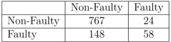
From Table 2.7, it can be observed that in case of navies Bayes technique,

total number of 835 (767+68) classes were classified correctly with 83.75% accuracy rate.

From Table 2.8, it can be observed that in case of SVM technique, total

num-ber of 848 (769+79) classes were classified correctly with 85.06% accuracy rate.

Table 2.4: After applying Linear Regression Non-Faulty Faulty Non-Faulty 725 66 Faulty 99 107

Table 2.5: After applying Polynomial Regression Non-Faulty Faulty

Non-Faulty 767 24 Faulty 148 58

(35)

Table 2.6: After applying Logistic Regression Non-Faulty Faulty Non-Faulty 771 20 Faulty 141 65 Table 2.7: After applying Naive Bayes

Non-Faulty Faulty Non-Faulty 767 24 Faulty 146 60 Table 2.8: After applying SVM

Non-Faulty Faulty Non-Faulty 791 0 Faulty 186 20

Table 2.9, lists the values of obtained performance parameters for Ellipse JDT core data set for the applied techniques. From Table 2.9, it can inferred that:

Logistics regression technique obtained promising classification rate when

compared to other four techniques, and also

It can be concluded that NEcost was less than 1 for the jdt data set for all

the five techniques. Logistic regression incurred negligibly less NEcost in comparison to other techniques.

Table 2.9: Result of experiment for Eclipse JDT Core

Technique Specification Recall Precision F-Measure Accuracy NEcost Linear regression 0.9166 0.8799 0.6185 0.8978 83.45 0.8943 Polynomial regression 0.9697 0.8383 0.7073 0.8992 82.75 0.8879 Logistics regression 0.9747 0.8454 0.7647 0.9055 83.85 0.8823 Naives Bayes 0.9697 0.8401 0.7143 0.9002 82.95 0.8871 SVM 1 0.8096 1 0.8948 81.34 0.8886 23

(36)

2.6 Summary Effectiveness of fault prediction Techniques

2.6 Summary

Prediction models are used to classify fault prone classes as faulty or not faulty, but less significance has been given on the usefulness of fault prediction, which is the need of the day for researchers as well as practitioners. So cost based measures related to fault prediction needs to be modeled. In this chapter, five different prediction techniques i.e., linear regression, polynomial regression, logistic regression, Naive Bayes and SVM were applied for fault prediction. Also a note on whether using these techniques for fault prediction is useful or not in terms of cost measure was presented.

The implementation process is carried out for a case study of Ellipse JDT core. The results are generated using MATLAB. Here normalized data set of CK metrics suite was used as requisite input to the prediction models. In this study, the results suggest that, fault prediction can be useful for the projects with percentage of faulty module less than certain threshold .

(37)

Neural Network for Fault Prediction

Introduction Reserch Background Proposed work Results Summary

(38)

Chapter 3 Neural Network for Fault

Prediction

3.1 Introduction

Experimental validation of software metrics in fault prediction for Object-Oriented methods using statistical and machine learning methods is necessary. By the process of validation the quality of software product in a software organization is ensured. Object-Oriented metrics play a crucial role in predicting faults. In literature, prediction models are mostly developed using statistical models. Neural networks (NN) have seen an explosion of interest over the years, and are being successfully applied across a range of problem domains. Indeed, anywhere that there are problems of classification and prediction, neural networks are being used, Neural network can be used as a prediction model because it enables modeling of complex functions. In this study, artificial neural network (ANN) with Gradient Descent and Levenberg Marquardt (LM) learning methods have been used to design a classifier to classify a class as faulty or not faulty. Chidamber and Kemerer (CK) metrics suite has been considered to provide requisite input data to design the model. A case study of Eclipse JDT core has been considered for predicting a comparative study of performances of three approaches. Fault prediction is found to be useful where normalized estimated fault removal cost (NEcost) was less than certain threshold value.

(39)

3.2 RESEARCH BACKGROUND Neural Network for Fault Prediction

3.2 RESEARCH BACKGROUND

The following sub-sections highlight on the data set being used for fault predic-tion. Data was normalized to obtain better accuracy and then dependent and independent variables are chosen for fault prediction.

3.2.1 Empirical data collection

Metric suites are used and defined for different goals such as fault prediction, effort estimation, re-usability and maintenance. In this study, the mostly commonly used CK metric suite [27] is used for fault prediction. The metric values of the suite were extracted using CKJM tool. In this study, NASA and PROMISE [28] datasets are used to evaluate the impact of fault-prediction techniques over the fault removal cost using proposed model (NEcost).

3.2.2 Dependent and independent variables

3.2.3 Case study

In this study, to analyze the effectiveness of the proposed approach, Ellipse JDT core was used as a case study.

3.2.4 Fault Data

To perform statistical analysis, bugs were collected from Promise data repository [28]. Table 2.1 shows the distribution of bugs based on the number of occurrence

(40)

3.2 RESEARCH BACKGROUND Neural Network for Fault Prediction

(in terms of percentage of class containing number of bugs) for Ellipse JDT core.

3.2.5 Descriptive statistics and correlation analysis

This subsection gives the comparative analysis of the fault data, descriptive statis-tics of classes and the correlation among the six metrics with that of Basili et al. [13]. Basili et al. studied Object-Oriented systems written in C++ language. They used the same CK metric suite. Logistic regression technique was employed to analyze the relationship between metrics and the fault proneness of classes

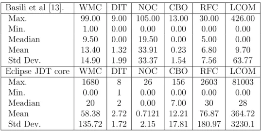
Table 3.1: Descriptive Statistics of Classes

Basili et al [13]. WMC DIT NOC CBO RFC LCOM Max. 99.00 9.00 105.00 13.00 30.00 426.00 Min. 1.00 0.00 0.00 0.00 0.00 0.00 Meadian 9.50 0.00 19.50 0.00 5.00 0.00 Mean 13.40 1.32 33.91 0.23 6.80 9.70 Std Dev. 14.90 1.99 33.37 1.54 7.56 63.77 Eclipse JDT core WMC DIT NOC CBO RFC LCOM

Max. 1680 8 26 156 2603 81003 Min. 0.00 1 0.00 0.00 0.00 0.00 Meadian 20 2 0.00 7.00 30 28 Mean 58.38 2.72 0.7121 12.21 76.87 364.72 Std Dev. 135.72 1.72 2.15 17.81 180.97 3230.1

The obtained CK metric values of Ellipse JDT core are compared with the results of Basili et al. [13]. In comparison with Basili et al. the total number of classes considered is much greater i.e., 997 classes were considered (Vs. 180 as used by Basiliet al.). Table 3.1 shows the statistical analysis of Basili et al project and Ellipse JDT core for CK Metric indicating Max, Min, Median and Standard deviation.

From Table 3.1, minimum values are almost same. But the maximum values are changes i.e., in Basili et al [13]. Maximum value of WMC is 99 but in our study, Maximum value is 1680. From Table 3.1, it is clear that the DIT metric has low value of mean and median for Eclipse JDT core. The low value of mean and median for DIT shows that inheritance was not consider much in both software system.

(41)

3.3 Proposed work for fault prediction Neural Network for Fault Prediction

Table 3.2: Correlations between the Metrics of Basili et al (lower) and Ellipse JDT core (upper)

WMC DIT NOC CBO RFC LCOM WMC 1.00 -0.123 0.084 0.602 0.8750 0.5123 DIT 0.02 1.00 -0.051 -0.111 -0.099 -0.055 NOC 0.24 0.00 1.00 0.2753 0.0765 0.0128 CBO 0.00 0.00 0.00 1.00 0.6133 0.39 RFC 0.13 0.00 0.00 0.31 1.00 0.6642 LCOM 0.38 0.00 0.00 0.01 0.09 1.00

The dependency between metrics is computed usingP earson’scorrelations (r: Coefficient of correlation) for Ellipse JDT core. The coefficient of correlation, r, is useful because it measures the strength and direction of the linear relationship between two variables. It is defined as the covariance of the variables divided by the product of their standard deviations. It also measures that allows us to determine how certain one can be in making predictions from a certain model. Table 3.2 shows the P earson’s correlation analysis for the dataset. The upper triangular matrix represents the correlations between the metrics in the Ellipse JDT core data set, and the lower triangular matrix represents the correlations between the metrics in the Basiliet al use data sets. Correlation obtained between WMC and RFC is 0.8750 which is highly correlated i.e., these two metrics are very much linearly dependent on each other, and correlation between NOC and RFC is 0.0765 which indicates that they are loosely correlated i.e., there is low dependency between these two metrics.

3.3 Proposed work for fault prediction

The following sub-sections highlight on the various neural network methods used for fault classification.

3.3.1 Data normalization

Input feature values were normalized over the range [0,1], so as to adjust the defined range of input feature value and avoid the saturation of neurons. In literature, techniques such as Min-Mx normalization, Z-Score normalization and

(42)

Decimal scaling are available for normalizing the data. In this study Min-Max normalization [33] technique has been used to normalize the data.

Min-Max normalization performs a linear transformation on the original data. It maps each of the actual dataxi of attributeX to normalized valuex′i which lies

in the range of [0,1]. The Min-Max normalization is calculated by using equation:

N ormalized(xi) =x′i =

xi−min(X)

max(X)−min(X) (3.2) where max(X) and min(X) represent the maximum and minimum value of the attribute X respectively.

3.3.2 Artificial neural network (ANN) model

ANN is used for solving problems such as classification and estimation [34]. In this study, ANN is used for design the model for predicting software fault using software metrics.

Input layer Hidden layer

Output layer

Figure 3.1: Artificial neural network

Figure 3.1 shows the architecture of ANN, which contains three layers i.e., input layer, hidden layer and output layer. Here, for input layer, linear activation function is used i.e., the output of the input layer is treated as input of the input layer. It is represented as:

(43)

For hidden and output layer, sigmoidal function or squashed-S function is used. The output of hidden layer ‘O′

h for input of hidden layer ‘Ih′ is represented as:

Oh=

1

1 +e−Ih (3.4)

and output of the output layer ‘O′

o for the input of the output layer ‘Oi′ is

repre-sented as:

Oo =

1

1 +e−Oi (3.5)

Neural network can be represented as:

Y′ ₌_f₍_{W, X}₎ _(3.6)

where Y′

is the output vector, X is the input vector, and W is the weight vector. The weight vector W is updated in every iteration so as to reduce Mean Square Error (MSE). MSE is based on:

M SE = 1 n n X i=1 (y′ i−yi)2 (3.7)

where y is the actual output and y′

is the expected output.

Different methods are available in literature to update weight vector ‘W’ such as: Gradient descent, Newton’s method, Quasi-Newton method, Gauss Newton conjugate-gradient method and Levenberg Marquardt method etc. In this study, Gradient descent and Levenberg Marquardt are used for updating the weights vector W.

Gradient descent method

Gradient descent is one of the method for updating the weights during learning phase [35]. Gradient descent method uses first-order derivative of total error to find the minima in error space. Normally Gradient vector G is defined as the 1st order derivative of error function Ek and error function is represented as:

Ek =

1 2(y

′

k−yk)2 (3.8)

Gradient vector G is given as:

G= d dW(Ek) = d dW( 1 2(y ′ k−yk)2) (3.9) 31

(44)

After computing the value of gradient vector G in each iteration, weighted vector W is updated as:

Wk+1=Wk−αGk (3.10)

where Wk+1 is the updated weights, Wk is the current weights, Gk is gradient

vector and α is the learning constant.

Levenberg Marquardt (LM) method

Levenberg Marquardt method locates the minimum of multivariate function in an iterative manner. It is expressed as the sum of squares of non-linear real-valued functions [36]. This method is used for updating the weights during learning phase. It is fast and stable in terms of its executions as it is a combination of steepest descent and Gauss Newton method. In Levenberg Marquardt the weights vector

W is updated as:

Wk+1 =Wk−(JkTJk+µI)−1Jkek (3.11)

whereWk+1 is the updated weights,Wkis the current weights, I is the identity

or unit matrix,J is the Jacobian matrix andµis always positive, called combina-tion coefficient i.e., when µis very small it act as a Gauss Newton method and if

µis very large then it as a Gradient descent method. Jacobian matrix is represented as:

J=             d dW1(E1,1) d dW2(E1,1) · · · d dWN(E1,1) d dW1(E1,2) d dW2(E1,2) · · · d dWN(E1,2) .. . ... ... ... d dW1(EP,M) d dW2(EP,M) · · · d dWN(EP,M)            

where N is number of weights, P is the number of input patterns, and M is the number of output patterns.

(45)

3.4 RESULTS Neural Network for Fault Prediction

3.4 RESULTS

In this section, the relationship between value of metrics and the fault found in a class is determined i.e., in all AI techniques six CK metrics are considered as input nodes and the output is the fault in the software.

The following steps are followed to design a classifier to predict faulty and non-faulty module in the software:

Step 1. Data Collection:

Data is extracted from Promise data repository.

Step 2. Normalized the dataset

Normalize the dataset over the range [0,1] using Min-Max normalization [Equation 3.2].

Step 3. Division of dataset into categories

Input data is divided into three categories i.e. training, validation and test set.

Step 4. Model design

The model is designed considering input dataset and output dataset.

Step 5. Training of network and updating Weights

Training data set is fed into the model to train the network and weights are updated using learning algorithm.

Step 6. Error calculation

Check the performance of the model. If satisfactory then stop, else again go to Step 5, update the weights and then proceed.

Step 7. Validation

Trained model will be validated by giving the validation set data. 33

(46)

Step 8. Testing

Finally the model is tested by feeding test set data.

3.4.1 Artificial Neural Network

ANN is an interconnected group of nodes. In this study, three layers of ANN are considered, in which six nodes act as input nodes, nine nodes represent the hidden nodes and one node acts as output node. ANN is a three phase network; the phases are used for learning, validation and testing purposes. So in this article 70% of total input pattern is considered for learning phase, 15% for validation and the rest 15% for testing. In this study six CK metrics are taken as input, and output is the fault prediction accuracy rate. The network is trained using Gradient descent method and Levenberg Marquardt method.

Gradient descent method

Gradient descent method is used for updating the weights using Equation 3.9 and 3.10. Table 3.3 to Table 3.4 show the classification matrix for jdt data set before and after applying ANN.

Table 3.3: Before applying ANN Not-Faulty Faulty Not-Faulty 791 0 Faulty 206 0

Table 3.4: After applying ANN Not-Faulty Faulty Not-Faulty 790 1 Faulty 261 45

From Table 3.3 it is clear that before applying the logistic regression analysis, a total number of 791 classes contained zero bugs and 206 classes contained at least one bug. But after applying ANN with gradient descent method learning method, total number of 790+45 classes are classified correctly with accuracy of 83.75%.

(47)

Figure 3.2 shows the graph plot for variation of mean square error values against no. of epoch (iteration).

0 100 200 300 400 500 600 700 800 900 1000 0.16 0.161 0.162 0.163 0.164 0.165 0.166 0.67 0.168 0.169 0.170 0.171 0.172 0.173 0.174 0.175 Iteration No.

Mean Square Error

Figure 3.2: Mean square error Vs No. of iteration

Levenberg marquardt method

Levenberg marquardt method is the technique for updating weights. In case of Gradient descent method, learning rateαis constant but in Levenberg marquardt method learning rate α varies in every iteration and it consume less iteration to train the network. Table 3.3 to Table 3.5 show the classification matrix for eclipse jdt core data set before and after applying ANN with Levenberg marquardt learning method.

Table 3.5: After applying ANN Not-Faulty Faulty Not-Faulty 741 50 Faulty 142 64

From Table 3.3 it is clear that before applying the logistic regression analysis, a total number of 791 classes contained zero bugs and 206 classes contained at

1 1.2 1.4 1.6 1.8 2 2.2 2.4 2.6 2.8 3 0.08 0.09 0.1 0.11 0.12 0.13 0.14 0.15 0.16 Iteration No.

Mean Square error

Figure 3.3: Mean square error Vs No. of iteration 35

(48)

least one bug. But after applying ANN with gradient descent method learning method, total number of 741+64 classes are classified correctly with accuracy of 80.74%. Figure 3.3 shows the graph plot for variation of mean square error values against no. of epoch or iteration. LM consumed only 3 iterations when compared with Gradient descent method which took 1000 iterations.

3.4.2 Fault removal cost evaluation

In this cost evaluation model, the data set of Eclipse JDT core from PROMISE repository was considered to evaluate the impact of fault prediction technique over the fault removal cost using the proposed model for computing NEcost. To illustrate effectiveness of our model, ANN classification techniques is considered. The goal is to demonstrate the cost evaluation model and suggest whether fault prediction using particular prediction technique is useful or not rather than iden-tifying the “best” fault-prediction technique. Figure 2.1 shows the block diagram for cost evaluation model.

Table 3.6 shows the various parameters related to cost evaluation model along with NEcost. NEcost is the evaluation criteria used in evaluating a prediction techniques usefulness in fault prediction. From Table 3.6, it is evident that RBFN approach took less fault removal cost (0.8952) when compared with other ap-proaches. From the result obtained using cost evaluation model it can be sug-gested that the selection of a fault-prediction technique does not only depend on the accuracy rate but it should also take into account the economics (fault removal cost) of software. However, while developing business critical applications, where ignoring faults can be crucial, then using fault prediction is not applicable; if it has high false negatives. Otherwise, it may result in a poor quality outcome.

Cost based evaluation model proposed in this study, answers two main ques-tions which are as follows:

i. Which fault prediction model is suitable among the applied techniques. ii. For a given software product, whether performing fault prediction analysis

(49)

3.5 Summary Neural Network for Fault Prediction

Table 3.6: Fault removal cost for Eclipse JDT core

Specification Recall Precision F-Measure Accuracy NEcost ANN (GD) 0.9987 0.8307 0.9783 0.9070 83.75 0.8785 ANN (LM) 0.9368 0.8392 0.5614 0.8853 80.74 0.9024

3.5 Summary

System analyst use prediction models to classify fault prone class as faulty or not faulty, which is the need of the day for researchers as well as practitioners. So more reliable approaches for prediction needs to be modeled. In this study, ANN was applied for fault prediction. The application of machine learning methods in fault prediction requires enormous amount of data and analyzing this huge amount of data is necessary with the help of a better prediction model.

Fault classification using these approaches was carried out for the Eclipse JDT core case study, by coding in MATLAB environment. ANN with gradient de-scent learning method obtained better fault classification when compared with the Levenberg Marquardt (LM) learning method. So from the proposed work of cost evaluation model, it can be noted that it is better to perform fault prediction when NEcost is less than one.

(50)

Hybrid ANN for Fault Prediction

Introduction Reserch Background Proposed work Results Summary

(51)

Chapter 4 Hybrid ANN for Fault Prediction

4.1 Introduction

Estimation of different parameters for Object-Oriented systems such as effort, quality and risk is of major concern in software development life cycle. Major-ity of the approaches available in literature for estimation and classification are based on statistical analysis and neural network techniques. Also it is perceive that numerous software metrics are consider as input for estimation. In this work, Chidamber and Kemerer metrics suite has been considered as a input data to design the classifier for classifying faulty and non-faulty module. Three artificial intelligence (AI) techniques such as: hybrid approach of neural network and ge-netics algorithm (Neuro-GA and adaptive Neuro-GA), hybrid approach of neural network and Particle Swarm Optimization (Neuro-PSO and Modified Neuro-PSO) and hybrid approach of neural network and Clonal Selection Algorithm (Neuro-CSA ) are used for fault classification. A case study of Eclipse JDT core has been considered for predicting a comparative study of performances of three ap-proaches. Fault prediction is found to be useful where normalized estimated fault removal cost (NEcost) was less than certain threshold value. It is observed from the obtained results that, Adaptive Neuro-GA model obtained promising results in terms of cost analysis when compared with other techniques.

(52)

4.2 Research background Hybrid ANN for Fault Prediction

4.2 Research background

The following sub-sections highlight on the data set being used for fault predic-tion. Data are normalized to obtain better accuracy and then dependent and independent variables are chosen for fault prediction.

4.2.1 Empirical data collection

Metric suites are used and defined for different goals such as fault prediction, effort estimation, re-usability and maintenance. In this study, the most commonly used metric i.e., CK metric suite [27] is used for fault prediction. The metric values of the suite are extracted using CKJM tool. This tool is being used to extract metric values for Eclipse JDT core available in the Promise data repository [28]. The CK metric values of the Eclipse JDT core are used for fault prediction.

4.2.2 Dependent and independent variables

4.3 Proposed work for fault prediction

The following sub-sections highlight on the various machine learning methods used for fault classification.

4.3.1 Neural Network (NN) Model

(53)

4.3 Proposed work for fault prediction Hybrid ANN for Fault Prediction

computational model for neural networks based on mathematics and algorithms [34]. This computational features involved in NN architecture can be very well applied for fault prediction.

Neuro-GA Approach

Neuro-GA is a hybrid approach of ANN and GA [37]. In this approach, genetic algorithm is used for updating the weight during learning phase. A neural network with a configuration of ‘l-m-n’ is considered for estimation i.e., the network consists of ‘l’ number of input neurons, ‘m’ number of hidden neurons, and ‘n’ number of output neurons. The number of weights N required for this network can be computed using the following equation:

N = (l+n)∗m (4.2) with each weight (gene) being a real number and assuming the number of digits (gene length) in weights to be d. The length of the chromosome L is computed using the following equation:

L=N ∗d = (l+n)∗m∗d (4.3) For determining the fitness value of each chromosome, weights are extracted from each chromosome using the following equation:

Wk=                                  if 0<=xkd+1 <5 −xkd+2∗10d−2₊_x kd+3∗10d−3₊_....₊_x (k+1)d 10d−2 if 5<=xkd+1 <= 9 +xkd+2∗10d−2₊_x kd+3∗10d−3₊_....₊_x (k+1)d 10d−2 (4.4)

The fitness values of each chromosome is determined based on the derived fitness function. The algorithm for deriving fitness function is as follows:

Let ¯(Ii,T¯i) ; i=1,2,3....,N where

Software fault prediction using object-oriented metrics

Software Fault Prediction

using

Object-Oriented Metrics

Lov Kumar

Department of Computer Science and Engineering

National Institute of Technology Rourkela

Rourkela-769008, Odisha, India

June 2014

Software Fault Prediction

using

Object-Oriented Metrics

Master of Technology

Computer Science and Engineering

Lov Kumar

Prof. S. K. Rath

Department of Computer Science and Engineering

National Institute of Technology Rourkela

Rourkela, Odisha, 769 008, India

Department of Computer Science and Engineering

National Institute of Technology Rourkela

Rourkela-769 008, Odisha, India.

Certificate

Acknowledgment

Abstract

Contents

List of Figures

List of Tables

List Of Abbreviation

Introduction

Chapter 1

Introduction

1.1

Literature Review

1.2

Software Metrics

1.3

Performance evaluation parameters

1.4

Motivation

1.5

Thesis Organization

Effectiveness of fault prediction Techniques

Chapter 2

Effectiveness of fault prediction

Techniques

2.1

Introduction

2.2

RESEARCH BACKGROUND

2.2.1

Empirical data collection

2.2.2

Dependent and independent variables

2.2.3

Case study

2.2.4

Fault Data

2.3

Proposed work for fault prediction

2.3.1

Linear Regression models

2.3.2

Polynomial regression models

2.3.3

Logistic regression model

2.3.4

Naive Bayes model

2.3.5

Support Vector Machine model

2.4

Cost analysis model

2.5

Experimental study

2.5.1

Experiment execution

2.5.2

Result and Analysis

2.6

Summary