FULL-LENGTH ARTICLE
Classification of Clustered Microcalcifications
using MLFFBP-ANN and SVM
Baljit Singh Khehra
a,*, Amar Partap Singh Pharwaha
b,1a
Department of Computer Science & Engineering, Baba Banda Singh Bahadur Engineering College, Fatehgarh Sahib 140407, Punjab, India
b
Department of Electronics and Communication Engineering, Sant Longowal Institute of Engineering and Technology, Longowal 148106, Sangrur, Punjab, India
Received 26 March 2015; revised 26 July 2015; accepted 16 August 2015 Available online 14 September 2015
KEYWORDS
Computer-Aided Diagnosis; Clustered Microcalcifications; LM-MLFFBP-ANN; SMO-SVM;
Confusion matrix and ROC analysis
Abstract The classifier is the last phase of Computer-Aided Diagnosis (CAD) system that is aimed at classifying Clustered Microcalcifications (MCCs). Classifier classifies MCCs into two classes. One class is benign and other is malignant. This classification is done based on some meaningful features that are extracted from enhanced mammogram. A number of classifiers have been proposed for CAD system to classify MCCs as benign or malignant. Recently, researchers have used Artificial Neu-ral Networks (ANNs) as classifiers for many applications. Multilayer Feed-Forward Backpropaga-tion (MLFFB) is the most important ANN that has been successfully used by researchers to solve various problems. Similarly, Support Vector Machines (SVMs) belong to another category of classi-fiers that researchers have recently given considerable attention. So, to explore MLFFB and SVM clas-sifiers for MCCs classification problem, in this paper, Levenberg-Marquardt Multilayer Feed-Forward Backpropagation ANN (LM-MLFFB-ANN) and Sequential Minimal Optimization (SMO) based SVM (SMO-SVM) are used for the classification of MCCs. Thus, a comparative evalu-ation of the relative performance of LM-MLFFBP-ANN and SMO-SVM is investigated to classify MCCs as benign or malignant. For this comparative evaluation, first suitable features are extracted from mammogram images of DDSM database. After this, suitable features are selected using Particle Swarm Optimization (PSO). At the end, MCCs are classified using LM-MLFFBP-ANN and SMO-SVM classifiers based on the selected features. Confusion matrix and ROC analysis are used to
* Corresponding author. Tel.: +91 9463446505.
E-mail addresses:[email protected](B.S. Khehra),[email protected](A.P.S. Pharwaha).
1 Tel.: +91 9463122255.
Peer review under responsibility of Faculty of Computers and Information, Cairo University.
Production and hosting by Elsevier
Egyptian Informatics Journal (2016)17, 11–20
Cairo University
Egyptian Informatics Journal
www.elsevier.com/locate/eijwww.sciencedirect.com
http://dx.doi.org/10.1016/j.eij.2015.08.001
1110-8665Ó2015 Production and hosting by Elsevier B.V. on behalf of Faculty of Computers and Information, Cairo University.
measure the performance of LM-MLFFBP-ANN and SMO-SVM classifiers. Experimental results indicate that the performance of SMO-SVM is better than that of LM-MLFFBP-ANN.
1. Introduction
Breast cancer that occurs among women in both developed and developing countries is one of the most dangerous dis-eases. It is difficult to prevent it but early detection is the key for reducing the mortality rate. Mammography is one of the most effective imaging techniques for early detection of breast cancer[1]. Clusters of Microcalcifications (MCCs), mass lesions, distortion in breast architecture and asymmetry between breasts are various types of breast abnormalities that are partially detected from mammograms. Clusters of Micro-calcifications (MCCs) are the most frequent symptoms of Duc-tal Carcinoma in Situ (DCIS). DCIS is one of various types of breast cancers[2]. Although mammography is frequently used in both developed and developing countries for breast cancer detection, but un-correct reading of mammogram is a prob-lem. This type of problem is occurred due to human error. Un-correct readings of mammogram are called false positive and false negative readings of mammogram. Due to false pos-itive detection, the need of unnecessary biopsy occurs while due to false negative detection, an actual tumor remains unde-tected. Thus, false positive and false negative readings of mam-mogram are main causes of unnecessary biopsy and missing the best treatment time. In fact, the need of the hour is to develop Computer-Aided Diagnosis (CAD) system for improving diagnosis accuracy of early breast carcinoma which would prevent unnecessary biopsy and not miss the best treat-ment time. The classifier is the last phase of CAD system that is aimed to classify MCCs as benign or malignant. For this, first mammogram images are enhanced. After this, features are extracted from enhanced mammogram. Then, a suitable set of features is searched from extracted features. At the end, classifiers classify MCCs based on suitable set of features. Recently, various researchers have applied a variety of classi-fiers for CAD system to classify MCCs as benign or malignant. Kramer and Aghdasi[3]used multi-scale statistical texture fea-tures to classify MCs in digitized mammograms using K-Nearest Neighbor (KNN) classifier. Bruce and Adhami [4] classified mammographic masses into stellate, nodular and round using Linear Discriminant Analysis (LDA) classifier. Bottema and Slavotinek[5]classified lobular and DCIS (small cell) MCs in digital mammograms using decision trees. In 2007, Bayesian network classifiers are used by Nicandro et al.[6]for the diagnosis of breast cancer. Fuzzy rough sets hybrid scheme is used by Hassanien[1]for breast cancer detec-tion. For classification of MCs as benign or malignant, Artifi-cial Neural Networks (ANNs) have been widely used [7–9]. Multilayer Feed-Forward Backpropagation (MLFFB) is the most important ANN that has been applied successfully to solve many problems [10–12]. Support Vector Machines (SVMs) have also been recently used to solve many problems [2,13–16]. SVMs are based on statistical learning theory. In the proposed research work, LM-MLFFBP-ANN and SMO-SVM are explored to classify MCCs as benign or malignant.
Experiments are performed on mammogram images of DDSM database[17].
2. Artificial Neural Network
An ANN is a computational model that is commonly used in situations when the knowledge is not properly defined and there is a need to solve non-linear complex problems. Multi-layer Feed-Forward Neural Network trained with Backpropa-gation algorithm is widely used for non-linear classification problems [18]. Multilayer Feed-Forward Backpropagation Artificial Neural Network (MLFFBP-ANN) is treated as a nested sigmoid scheme. Therefore, the following equation is used to represent the output function of ANN[19]:
FðxiÞ ¼FNðWN ðFN1ð. . .F2ðW2F1ðW1x1þB1Þ
þB2Þ. . .Þ þBN1Þ þBNÞ ð1Þ
where Nis total layers of Artificial Neural Network;B1,B2,
. . .,BNare the bias vectors; W1,W2,. . .,WNare the weight
vectors and F1, F2, . . ., FN are activation transfer functions
of layers.
In fact, studies on ANNs[20,21]have highlighted that the most often used ANN architecture is feed-forward network designed around multilayer topologies with Backpropagation learning algorithm. In the feed-forward ANN, a neuron trans-fers data to the neuron of the next layer through a function called activation function that may be the sigmoid or linear one[22]. When sigmoid activation function is used, the output of thejth neuron is calculated as
zj¼
1
1þerðz injÞ ð2Þ
wherez injis the input of thejth neuron received from the
neu-rons of the previous layer calculated as z inj¼bjþ
Xn i¼1
xiwij ð3Þ
wherexiis the output ofith neuron of the previous layer;nis
the total number of neurons in the previous layer; wij is the
connection weight of thejth neuron withith neuron of the pre-vious layer;bjis thejth neuron bias andrdefines the steepness
of the sigmoid activation function.
In the learning phase,wij andbjvalues are updated using
the following equations[23]:
wijðnewÞ ¼wijðoldÞ þDwij ð4Þ
bjðnewÞ ¼bjðoldÞ þDbj ð5Þ
Dwij¼adjxi ð6Þ
Dbj¼adj ð7Þ
whereais the learning rate anddis correction factor. The per-formance of ANN is evaluated by Mean Square Error (MSE) that is defined as
Ó2015 Production and hosting by Elsevier B.V. on behalf of Faculty of Computers and Information,
Cairo University. This is an open access article under the CC BY-NC-ND license (http://creativecommons.
MSE¼ 1 L XL k¼1 Xm j¼1 ðtk j y k jÞ 2 ð8Þ whereL is the number of training pairs;mis the number of neurons in the output layer;yk
j andt k
j are the actual and target
outputs atjth neuron forkth training pair. 2.1. MLFFBP-ANN for classifying MCCs
Classification of MCCs as benign or malignant classes is a two-class pattern two-classification problem. LetXj2 ½x1;x2;x3;. . .;xi;
. . .;xnbe a set of features extracted from mammograms that
acts as input vector for MLFFBP-ANN andYj2 ½0;1be
out-put vector of MLFFBP-ANN. ‘0’ represents benign MCCs and ‘1’ represents malignant MCCs. Let Mj be one training set ofLsamples, i.e.Mj¼ ½ðX
j;YjÞ; j¼1;2;3;. . .;L.
Number of neurons in input layer (n) depends upon input vector and number of hidden neurons (p) is chosen experimen-tally. Number of neurons in output depends upon output vec-tor. Features are used as inputs of the neurons of input layer. Thus,nis number of features extracted from MCCs. Classifi-cation of MCCs is a two-class pattern classifiClassifi-cation problem. So, output layer has only one neuron to represent binary out-put. Neurons are interconnected with each other and a weight is assigned to each link for representing the link-strength between the neurons. In order to classify MCCs as benign or malignant, an attempt is made here to implement a MLFFBP-ANN based classifier to classify MCCs as benign or malignant. An algorithm is written using MATLAB pro-gramming. The implementation neural model comprises of a hidden layer of sigmoidal neurons that receives numeric values of features and broadcasts output values to a layer of linear neurons, which finally computes the network output. Using Eq.(2), the output ofjth neuron of hidden layer for the pro-posed model is computed by
zj¼tansig vojþ Xn i¼1 xivij ! ð9Þ wherenis the total number of neurons in input layer;vojis the
bias ofjth neuron of hidden layer;vijis the weight betweenith
neuron of input layer andjth neuron of hidden layer and tan sig(_s) is a hyper-tangent sigmoid activation transfer function. The output of the proposed MLFFBP-ANN model is com-puted as FANNðXjÞ ¼purelin wokþ Xp j¼1 zjwjk ! ð10Þ wherepis the total number of neurons in hidden layer;wokis
the bias of kth neuron of the output layer (in the proposed model,k= 1 because output layer has only one neuron); wjk
is the weight betweenjth neuron of hidden layer andkth neu-ron of the output layer; andpurelin(s) is linear activation trans-_ fer function.
The proposed MLFFBP-ANN model updates weights and biases values by means of an adaptive process which minimizes the output neurons errors using Eqs.(4)–(7)as follows: vijðnewÞ ¼vijðoldÞ þDvij ð11Þ Dvij¼adjxi ð12Þ vojðnewÞ ¼vojðoldÞ þDvoj ð13Þ Dvoj¼adj ð14Þ wjkðnewÞ ¼wjkðoldÞ þDwjk ð15Þ Dwjk¼adkzj ð16Þ wokðnewÞ ¼wokðoldÞ þDwok ð17Þ Dwok¼adk ð18Þ
wheredkis factor that is used to update weightswjkanddjis a
factor that is used to update weightsvij. Using Eq.(8), MSE
for the proposed model is calculated as MSE¼1 L XL j¼1 ½YjFANNðXjÞ 2 ð 19Þ During training, a set of numeric values of features of MCCs corresponding to the MCCs category is used to update the weights and biases of the neurons to minimize the output neuron error. However, the best ANN structure is not known in advance [18]. The best ANN structure depends upon the number of hid-den layers, number of neurons in each hidhid-den layer, activation function, learning algorithm and training parameters. To train MLFFBP-ANN, various training algorithms are available [24]. In the proposed research work, Levenberg-Marquardt training algorithm is considered to train MLFFBP-ANN for characterization of MCCs as benign or malignant.
3. Support Vector Machine
SVM is a two-class classifier developed by Vapnik[25]. Learn-ing of SVM is supervisLearn-ing learnLearn-ing that is based on statistical learning theory. Basic principal of SVM is structural risk min-imization. Structural risk minimization means to get a low error rate on unseen data set (outside training data set). For non-linear classification problems, kernel function based SVM is used. Kernel function converts non-linear classifica-tion problem to linear classificaclassifica-tion problem through mapping the input feature space to higher dimensional feature. After this, an optimal separating hyperplane is used to separate the two classes of the two-class pattern classification problem.
For classification of MCCs as benign or malignant, a set ofL training data samples is considered. Such set is denoted as fðXj;YjÞ; j¼1;2;. . .;Lg, whereXj is input data sample that
belongs to classYj2 fþ1;1g. Input data sample is represented
by a vectorX2 fxi;i¼1;2;. . .;ngin whichfxi;i¼1;2;. . .;ng
is a set ofnfeatures of the cluster of MCs and output is repre-sented asY2 fþ1;1g, where ‘+1’ is for malignant cluster of MCs and ‘1’ is for benign cluster of MCs. For separating the positive and negative classes, a separating hyperplane is used. Separating hyperplane should be optimal for correct classifica-tion of positive and negative classes. From the above discussion, the formulation of optimization problem to find optimal sepa-rating hyperplane can be stated as
Target: Minimize w
Tw
2
wherewis the norm to the hyperplane;kwkjbj is the perpendicular distance from the origin to hyperplane to the origin.
Thus, the main objective is to findwandbfor minimization ofwTw
2 along with the satisfaction of constraints. The optimal
values w* and b* are used to classify a test example Z as
follows:
classðZÞ ¼signðwTZþbÞ ð20Þ
The above defined problem belongs to Quadratic Program-ming (QP) optimization problem with linear constraints. Lagrangian formulation of the above said problem [26] is required to solve it. In Lagrangian formulation, objective func-tion is defined as LP¼ 1 2w TwX L j¼1 ajYjðwTXjþbÞ þ XL j¼1 aj ð21Þ Target: MinimizeLPw.r.tw,b Constraints:
(a) Derivatives ofLPwith respect to allajvanish
(b) ajP0
Dual formulation of the above primal problem is written as Target: MaximizeLP
Constraints:
(a) Gradient ofLPw.r.twandbvanishes
(b) ajP0
When gradient ofLPw.r.twandbis vanished, then the
fol-lowing conditions are occured:
w¼X L j¼1 ajYjXj ð22Þ XL j¼1 ajYj¼0 ð23Þ
From Eqs.(21)–(23), the following equation is obtained:
LD¼ XL j¼1 aj 1 2 XL j¼1 XL i¼1 ajaiYjYiXTjXi ð24Þ
Thus, new formulation of the problem is obtained as Target: MaximizeLD
Constraints: (a) PLj¼1ajYj¼0 (b) ajP0
Thus, the main objective is to finda1,a2,. . .,aLfor
maxi-mization of LD along with the satisfaction of constraints.
For non-zero aj; j¼1;2;. . .;Ls, the optimal values of w*
andb*are obtained as follows:
w¼X Ls j¼1 ajYjXj ð25Þ b¼Yj XLs j¼1 ajYjXTjXj ð26Þ
where non-zero Lagrange multipliers,aj; j¼1;2;. . .;Ls,
indi-cate their corresponding support vectors Sj2 ðXj;YjÞ. Thus,
the following equation is used to classify a test exampleZas classðZÞ ¼sign X Ls j¼1 ajYjXTjZþb ! ð27Þ 3.1. Karush–Kuhn–Tucker condition
Lagrangian formulation of the problem (LP) is a convex
min-imum QP optimization problem. Property of convex minimiza-tion problem is as follows: if a local minimum exists, then it is a global minimum[27]. Karush–Kuhn–Tucker condition[28] is sufficient when objective function is convex and solution space is also convex. According to this condition, gradient of the objective function of Lagrangian problem w.r.t w andb vanishes and multiplication of each Lagrangian multiplier with corresponding constraint is also zero for all Lagrangian multi-pliers greater than or equal to zero[29,30].
@LP @w ¼0)w¼ XL j¼1 ajYjXi ð28Þ @LP @b ¼0) XL j¼1 ajYj¼0 ð29Þ ajðYjðwTXjþbÞ 1Þ ¼0 8j ð30Þ ajP0 8j ð31Þ
The above equations are used to obtain optimal values of w*andb*.
3.2. Non-linear SVM classifier
For solving non-linear classification problems, non-linear SVM classifiers are used through kernel functions. Kernel function maps training input data of input space Rd onto a higher dimensional feature spaceHusing transformation oper-ator/ðÞ. This is done to separate training data points into two classes by a hyperplane[29].
/: Rd!H ð32Þ
Relation between kernel function K(Xj,Xi) and mapping
operator/ðÞ[31]is shown as KðXj;XiÞ ¼/ðXjÞ
T
/ðXiÞ 8Xj;Xi2Rd ð33Þ
Thus, dual form of the problem can be formulated as follows:
Find a1, a2, . . ., aL such that LD¼
PL j¼1aj12
PL j¼1
PL
i¼1ajaiYjYiKðXj;XiÞis maximized and
(a) PLj¼1ajYj¼0 (b) 06aj6Cfor8aj
For non-zeroaj; j¼1;2;. . .;Ls,w*is calculated from Eq.
(25)andb*is obtained as follows:
b¼Yj
XLs
j¼1
Thus, a test exampleZis classified as classðZÞ ¼sign X Ls j¼1 ajYjKðXj;ZÞ þb ! ð35Þ A most commonly used kernel function in SVM[32,33]is linear that is defined as follows:
Kðx;yÞ ¼xTy ð36Þ
3.3. Sequential Minimal Optimization for SVM
Sequential Minimal Optimization (SMO) [34] decomposes SVM-QP problem into QP sub-problems. At each step, the smallest possible optimization problem is selected for solving. For this, at each step, SMO selects two Lagrange multipliers. This is done to find the optimal values for Lagrange multipliers and SVM is updated to reflect the new optimal values. First, a Lagrange multiplier (a1) is selected that violates the Karush–
Kuhn–Tucker condition [28] for the optimization problem. After this, second Lagrange multiplier (a2) is selected and
opti-mizes the pair (a2,a2). This process is repeated to achieve the
convergence. The main advantage of SMO is that two Lagrange multipliers are solved analytically instead of entirely numerical QP optimization. In addition, no extra matrix is required for storage at all.
4. Measures for classifier accuracy
Confusion matrix[35]and ROC analysis[36]are two measures that are commonly used to find the accuracy of classifier to classify MCCs as benign and malignant. A confusion matrix evaluates the accuracy of classifier based on the actual and pre-dicted classifications done by a classifier. For a classifier and an instance, possible outcomes are four: true positive, true neg-ative, false positive and false negative. True positive is a cor-rect judgment of classifier about a malignant cluster of MCs while true negative is a correct judgment of classifier about a benign cluster of MCs. Similarly, false positive is a wrong judg-ment of classifier about a benign cluster of MCs while false negative is a wrong judgment of classifier about a malignant cluster of MCs. These possible outcomes of a classifier are shown inTable 1. Such table is called confusion matrix.
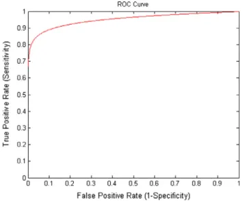
ROC analysis is another measure that is used to find the accuracy of classifier related to medical decision. In ROC anal-ysis, ROC curve is plotted to measure the accuracy of classifier. To plot ROC curve, 1-Specificityis taken along x-axis while Sensitivityis taken along y-axis and at various threshold set-tings, the curve is generated by plotting theSensitivityagainst the 1-Specificity. The meaning of 1-SpecificityisFalse Positive RatewhileSensitivityisTrue Positive Rate.
In case of confusion matrix, accuracy of classifier is found by using the following equation:
True Positive RateandFalse Positive Rateare defined as True Positive RateðSensitivityÞ ¼ TPs
TPsþFNs ð37Þ
False Positive Rateð1-SpecificityÞ ¼ FPs
TNsþFPs ð38Þ
where TPs are number of true positive decisions taken by classifier; TNs are number of true negative decisions taken
Table 1 Confusion matrix. Target
Positive Negative
Decision by classifier
Positive True positive False positive
Negative False negative True negative
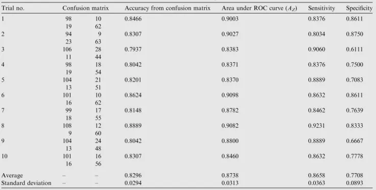
Table 2 Performance of LM-MLFFBP to classify MCCs in 10 random experimental trials.
Trial no. Confusion matrix Accuracy from confusion matrix Area under ROC curve (AZ) Sensitivity Specificity
1 98 10 0.8466 0.9003 0.8376 0.8611 19 62 2 94 9 0.8307 0.9027 0.8034 0.8750 23 63 3 106 28 0.7937 0.8383 0.9060 0.6111 11 44 4 98 18 0.8042 0.8371 0.8376 0.7500 19 54 5 104 21 0.8201 0.8370 0.8889 0.7083 13 51 6 101 10 0.8624 0.9098 0.8632 0.8611 16 62 7 99 17 0.8148 0.8782 0.8462 0.7639 18 55 8 108 12 0.8889 0.9082 0.9231 0.8333 9 60 9 104 24 0.8042 0.8800 0.8889 0.6667 13 48 10 101 16 0.8307 0.8460 0.8632 0.7778 16 56 Average – – 0.8296 0.8738 0.8658 0.7708 Standard deviation – – 0.0294 0.0313 0.0363 0.0893
by classifier;FNsare number of false negative decisions taken by classifier and FPs are number of false positive decisions taken by classifier.
In case of confusion matrix, accuracy of classifier is found by using the following equation:
Accuracy¼ TPsþTNs
TPsþFPsþTNsþFNs ð39Þ
In case of ROC analysis, the area under the ROC curve (AZ) is used to measure the accuracy of classifier[37].AZis
in the range between 0.0 and 1.0. So, AZ lies between 0.0
and 1.0. For 100% accuracy,AZ should be 1.0. Trapezoidal
rule or Simpson’s rule can be used to computeAZ.
According to Hosmer and Lemeshow [38], classifiers are divided into the following four categories based on the Accuracy:
If 0.56Accuracy< 0.6, then classifier is called fail classifier
If 0.66Accuracy< 0.7, then classifier is called poor classifier
If 0.76Accuracy< 0.8, then classifier is called fair classifier
If 0.86Accuracy< 0.9, then classifier is called good classifier
If 0.96Accuracy61.0, then classifier is called excellent classifier
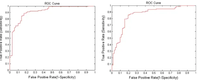
Figure 1 ROC curves of 1st and 10th random experimental trials of LM-MLFFBP classifier for classifying MCCs as benign and malignant.
Figure 2 Confusion matrices of 1st and 10th random experimental trials of LM-MLFFBP classifier for classifying MCCs as benign and malignant.
5. Experimental results and discussion
In order to explore LM-MLFFBP-ANN and SMO-SVM to classify MCCs as benign or malignant, experiments are per-formed on data extracted from mammogram images of DDSM database[17]. For comparative evaluation, confusion matrix
and ROC analysis are used. MATLAB 7.7 software is used for simulation.
5.1. Results of LM-MLFFBP-ANN
In order to find the performance of LM-MLFFBP for classify-ing MCCs as benign or malignant, different types of mammo-gram images are taken from standard benchmark digital database for screening mammography (DDSM) [17]. From mammogram images of DDSM database, a total of 380 suspi-cious regions are selected. From these samples, malignant sam-ples are 235 and benign samsam-ples are 145. A set of 50 features is extracted from suspicious regions [39]. After this, Particle Swarm Optimization (PSO) is used to select an optimal subset of 23 most suitable features from 50 extracted. Such optimal subset of features is used in LM-MLFFBP. In the architecture of LM-MLFFBP, one hidden layer is taken with 15 hidden units. The activation function between input layer and hidden layer is sigmoid while that between hidden layer and output layer is linear. Default values of different parameters are set according to MATLAB 7.7 environment. For training pur-pose, 191 samples are selected from 380 samples and the remaining samples (189) are used for testing purpose. For find-ing the performance of the classifier to classify MCCs as benign or malignant, 10 random experiment trials are per-formed. Confusion matrix and ROC analysis are used to mea-sure the performance of the trained classifier for classifying Clusters of MCs. Tabular results of 10 random experimental trials of LM-MLFFBP for classifying MCCs as benign or malignant in the form of accuracy calculated from confusion matrix and ROC analysis are shown inTable 2.Fig. 1 illus-trates ROC curves of first and last random experimental trials whileFig. 2illustrates confusion matrices of first and last ran-dom experimental trials.
Figure 3 Common ROC curve of 10 random experimental trials of LM-MLFFBP classifier for classifying MCCs as benign and malignant.
Table 3 Average accuracy of LM-MLFFBP in terms of confusion matrix and ROC analysis.
Average accuracy from confusion matrices Average accuracy from ROC curves Accuracy from common ROC curve Overall accuracy 0.8296 0.8738 0.8918 0.8651
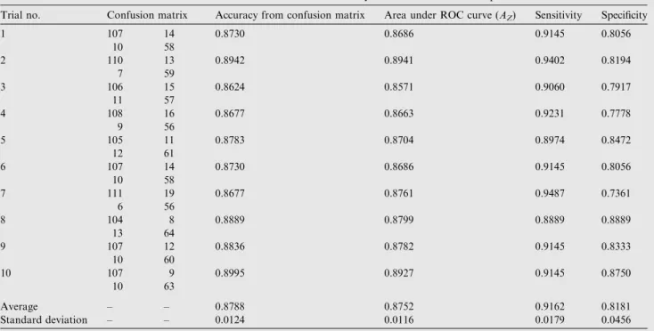
Table 4 Performance of SMO-SVM with linear kernel function to classify MCCs in 10 random experimental trials.
Trial no. Confusion matrix Accuracy from confusion matrix Area under ROC curve (AZ) Sensitivity Specificity
1 107 14 0.8730 0.8686 0.9145 0.8056 10 58 2 110 13 0.8942 0.8941 0.9402 0.8194 7 59 3 106 15 0.8624 0.8571 0.9060 0.7917 11 57 4 108 16 0.8677 0.8663 0.9231 0.7778 9 56 5 105 11 0.8783 0.8704 0.8974 0.8472 12 61 6 107 14 0.8730 0.8686 0.9145 0.8056 10 58 7 111 19 0.8677 0.8761 0.9487 0.7361 6 56 8 104 8 0.8889 0.8799 0.8889 0.8889 13 64 9 107 12 0.8836 0.8782 0.9145 0.8333 10 60 10 107 9 0.8995 0.8927 0.9145 0.8750 10 63 Average – – 0.8788 0.8752 0.9162 0.8181 Standard deviation – – 0.0124 0.0116 0.0179 0.0456
From confusion matrices, it is observed that the average accuracy is 0.8296 while from ROC analysis (average of all areas under ROC curves) the average accuracy is 0.8738. In ROC anal-ysis, Simpson’s rule is used to find area under ROC curve. Log-arithmic function is used to plot a common ROC curve of 10 random experimental trials. Common ROC curve is shown in Fig. 3. Accuracy from common ROC curve is 0.8918. The over-all accuracy of LM-MLFFBP is calculated through the average of the three accuracy measures (average accuracy from confu-sion matrices, average accuracy from ROC curve and accuracy from common ROC curve). Thus, the overall accuracy of LM-MLFFBP is 0.8651 that is shown inTable 3.
5.2. Results of SMO-SVM
Secondly, in order to explore the performance of SMO-SVM for classifying MCCs as benign or malignant, the same
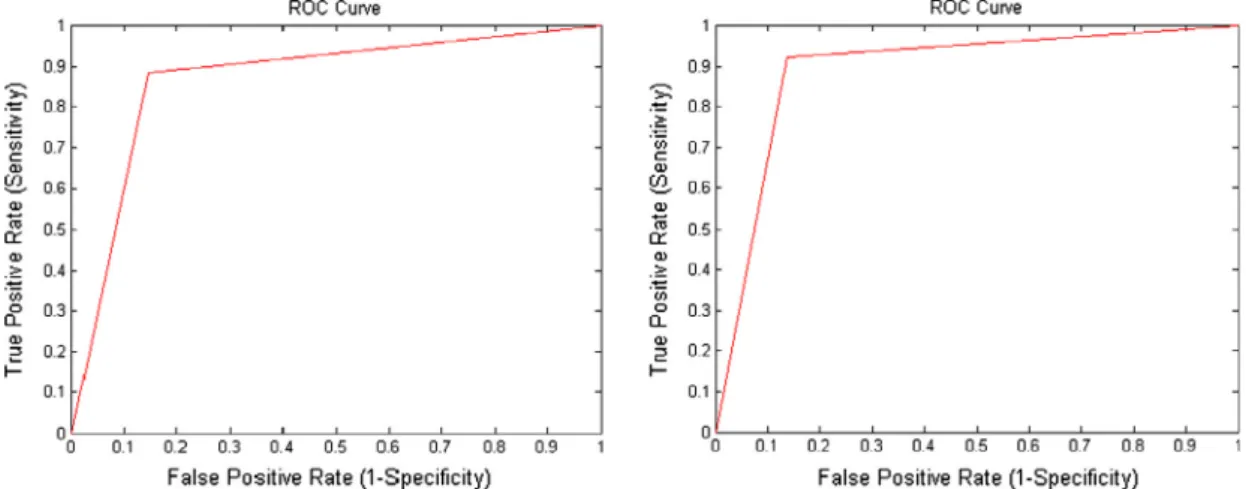
sam-ples that have been used for LM-MLFFBP are considered. The same 23 features are used that have been selected from 50 features by PSO for LM-MLFFBP. In this study, linear ker-nel function is considered. In the same way as used in LM-MLFFBP, the same 191 samples as used in LM-MLFFBP are used for training and the same 189 samples are used for testing purpose. Similarly, as in LM-MLFFBP, 10 random experimental trials are performed. Results of 10 random exper-imental trials in the form of confusion matrix and area under ROC curve are shown inTable 4.Fig. 4is used to show ROC curves of first and last random experimental trials whileFig. 5 illustrates confusion matrices of first and last experimental tri-als. From confusion matrix, the average accuracy of SMO-SVM classifier for classifying Clusters of MCs is 0.8788 while average accuracy of SMO-SVM classifier for classifying Clus-ters of MCs from ROC curves is 0.8752.Fig. 6illustrates com-mon ROC curve obtained from 10 random experimental trials.
Figure 4 ROC curves of 1st and 10th random experimental trials of SMO-SVM with linear kernel function classifier for classifying MCCs as benign and malignant.
Figure 5 Confusion matrices of 1st and 10th random experimental trials of SMO-SVM with linear kernel function classifier for classifying MCCs as benign and malignant.
Accuracy of SMO-SVM from ROC curve in terms of area under ROC curve is 0.9509. Thus, the overall accuracy of SVM with linear kernel function and SMO hyperplane finding method for classifying MCCs as benign or malignant is 0.9016 that is shown inTable 5.
6. Conclusion and future work
In this paper, an attempt is made to compare MLFFB-ANN and SVM classifiers to classify MCCs as benign or malignant. For this purpose, Levenberg-Marquardt training algorithm for MLFFB-ANN and Sequential Minimal Optimization hyper-plane finding method with linear kernel function for SVM are investigated. For this investigation, 10 random experiment trials are performed for LM-MLFFBP-ANN and SMO-SVM classifiers to classify MCCs as benign or malignant. From these experimental results, it is observed that LM-MLFFBP-ANN classifier belongs to good classifier category according to Hosmer and Lemeshow’s rule, while linear kernel function with SMO method based SVM classifier belongs to the excel-lent classifier category. Results of this study are quite promis-ing for selectpromis-ing a suitable classifier to classify MCCs as benign or malignant. Based on the results of simulation studies and experiments performed in this study, it is concluded that linear kernel function with SMO method based SVM classifier can be used as a classifier to classify MCCs as benign or malignant for achieving highest accuracy. This research work is very useful
for radiologists to characterize clusters of MCs in mammogram.
The results of the mentioned classifiers are encouraging and show good accuracy within experimental errors. But, in future to achieve above 91% overall accuracy, metaheuristic approaches can also be used to find the optimal hyperplane along with different kernel functions in SVM.
References
[1]Hassanien AE. Fuzzy rough sets hybrid scheme for breast cancer detection. Image Vis Comput 2007;25(2):172–83.
[2]Fu JC, Lee SK, Wong ST, Yeh JY, Wang AH, Wu HK. Image segmentation features selection and pattern classification for mammographic microcalcifications. Comput Med Imag Graph 2005;29(6):419–29.
[3] Kramer D, Aghdasi F. Classifications of microcalcifications in digitized mammograms using multiscale statistical texture analy-sis. In: Proc. South African symposium on communications and signal processing (COMSIG-98), Rondebosch, South African, 7–8 Sep.; 1998. p. 121–6.
[4]Bruce LM, Adhami RR. Classifying mammographic mass shapes using the wavelet transform modulus-maxima method. IEEE Trans Med Imag 1999;18(12):1170–7.
[5]Bottema MJ, Slavotinek JP. Detection and classification of lobular and DCIS (small cell) microcalcifications in digital mammograms. Pattern Recogn Lett 2000;21(13–14):1209–14. [6]Nicandro C-R, Hector GA-M, Humberto C-C, Luis AN-F, Rocio
EB-M. Diagnosis of breast cancer using Bayesian networks: a case study. Comput Biol Med 2007;37(11):1553–64.
[7]Christoyianni I, Koutras A, Dermatas E, Kokkinakis G. Com-puter aided diagnosis of breast cancer in digitized mammograms. Comput Med Imag Graph 2002;26(5):309–19.
[8]Halkiotis S, Botsis T, Rangoussi M. Automatic detection of clustered microcalcifications in digital mammograms using math-ematical morphology and neural networks. Signal Process 2007;87 ():1559–68.
[9]Mazurowski MA, Habas PA, Zurada JM, Lo JY, Baker JA, Tourassi GD. Training neural network classifiers for medical decision making: the effect of imbalanced datasets on classifica-tion performance. Neural Netw 2008;21(2–3):427–36.
[10]Delen D, Walker D, Kadam A. Predicting breast cancer surviv-ability: a comparison of three data mining methods. Artif Intell Med 2005;34(2):113–27.
[11]Singh AP, Kamal TS, Kumar S. Virtual curve tracer for estimation of static response characteristics of transducers. Measurement 2005;38(2):166–75.
[12]Varela C, Tahoces PG, Mendez AJ, Souto M, Vidal JJ. Computerized detection of breast masses in digitized mammo-grams. Comput Biol Med 2007;37(2):214–26.
[13]Arodz T, Kurdziel M, Sevre EOD, Yuen DA. Pattern recognition techniques for automatic detection of suspicious-looking anoma-lies in mammograms. Comput Methods Programs Biomed 2005;79(2):135–49.
[14]El-Naqa I, Yang Y, Wernick MN, Galatsanos NP, Nishikawa RM. A support vector machine approach for detection of microcalcifications. IEEE Trans Med Imag 2002;21(12):1552–63. [15]Mavroforakis ME, Georgiou HE, Dimitropoulos N, Cavouras D, Theodoridis S. Mammographic masses characterization based on localized texture and dataset fractal analysis using linear, neural and support vector machine classifiers. Artif Intell Med 2006;37 ():145–62.
[16]Wei L, Yang Y, Nishikawa RM. Microcalcification classification assisted by content-based image retrieval for breast cancer diagnosis. Pattern Recogn 2009;42(6):1126–32.
[17]http://marathon.csee.usf.edu/Mammography/Database.html.
Figure 6 Common ROC curve of 10 random experimental trials of SMO-SVM with linear kernel function for classifying MCCs as benign and malignant.
Table 5 Average accuracy of SMO-SVM with linear kernel function in terms of confusion matrix and ROC analysis.
Average accuracy from confusion matrices Average accuracy from ROC curves Accuracy from common ROC curve Overall accuracy 0.8788 0.8752 0.9509 0.9016
[18]Widrow B, Lehr MA. 30 Years of adaptive neural networks: perceptron, machine and backpropagation. Proc IEEE 1990;78 ():1415–42.
[19]Haykin S. Neural networks: a comprehensive foundation. 2nd ed. Delhi, India: Pearson Education, Inc.; 2004, p. 202.
[20] Bhowmick B, Pal NR, Pal S, Patel SK, Das J. Detection of microcalcification with neural networks. In: Proc. IEEE interna-tional conference on engineering of intelligent systems (ICEIS-06), Islamabad, Pakistan, 22–23 Apr.; 2006. p. 281–6.
[21]Cheng HD, Cui M. Mass lesion detection with a fuzzy neural network. Pattern Recogn 2004;37(6):1189–200.
[22]Haykin S. Neural networks and learning machines. 3rd ed. New Delhi: PHI; 2010, p. 691.
[23]Fausett L. Fundamentals of neural networks: architectures, algorithms, and applications. Englewood Cliffs (NJ, USA): Prentice-Hall, Inc.; 1994, p. 289.
[24]Hagan MT, Demuth HB, Beale M. Neural network design. USA: Thomson Learning; 1996, p. 2–11.
[25]Vapnik VN. The nature of statistical learning theory. 2nd ed. NY (USA): Springer-Verlag; 2000, p. 131.
[26]Rardin RL. Optimization in operation research. 2nd ed. Delhi, India: Pearson Education, Inc.; 2003, p. 810.
[27]Deb K. Optimization for engineering design: algorithms and examples. New Delhi, India: PHI; 2003, p. 77.
[28]Taha HA. Operation research: an introduction. 7th ed. New Delhi, India: Pearson Education, Inc.; 2006, p. 765.
[29]Burges CJC. A tutorial on support vector machines for pattern recognition. Data Min Knowl Disc 1998;2(2):121–67.
[30] Fletcher R. Practical methods of optimization. 2nd ed. NY (USA): John Wiley & Sons, Inc.; 1987, p. 219.
[31] Ayat NE, Cheriet M, Suen CY. Automatic model selection for the optimization of SVM kernels. Pattern Recogn 2005;38(10):1733–45. [32] Karatzoglou A, Meyer D, Hornik K. Support vector machines in
R. J Stat Softw 2006;15(9):1–28.
[33] Malon C, Uchida S, Suzuki M. Mathematical symbol recognition with support vector machines. Pattern Recogn Lett 2008;29 ():1326–32.
[34] Platt JC. Fast training of support vector machines using sequen-tial minimal optimization. In: Scholkopf Bernhard, Burges Christopher JC, Smola Alexander J, editors. Advances in Kernel methods: support vector learning. Cambridge (MA, USA): MIT Press; 1999. p. 185–208.
[35] Kohavi R, Provost F. Glossary of terms. J Mach Learn-Spec Issue Appl Mach Learn Knowl Discov Process 1998;30(2–3):271–4. [36] Fawcett T. An introduction to ROC analysis. Pattern Recogn Lett
2006;27(8):861–74.
[37] Karnan M, Thangavel K. Automatic detection of the breast border and nipple position on digital mammograms using genetic algorithm for asymmetry approach to detection of microcalcifi-cations. Comput Methods Programs Biomed 2007;87(1):12–20. [38] Hosmer DW, Lemeshow S. Applied logistic regression. 2nd ed. NJ
(USA): John Wiley & Sons, Inc.; 2000, p. 164.
[39] Khehra BS, Pharwaha APS. Least-squares support vector machine for characterization of clusters of microcalcifications. World Acad Sci, Eng Technol Int J Comput, Inform Sci Eng 2013;7(12):932–41.