ISSN 2042-2695
CEP Discussion Paper No 1302
September 2014
Assessing the Effect of School Days and Absences
on Test Score Performance
Abstract
While instructional time is viewed as crucial to learning, little is known about the effectiveness of
reducing absences relative to increasing the number of school days. In this regard, this paper jointly
estimates the effect of absences and length of the school calendar on test score performance. Using
administrative data from North Carolina public schools, we exploit a state policy that provides
variation in the number of days prior to standardized testing and find substantial differences between
these effects. Extending the school calendar by ten days increases math and reading test scores by
only 0.8% and 0.2% of a standard deviation, respectively; a similar reduction in absences would lead
to gains of 5.8% and 3% in math and reading. We perform a number of robustness checks including
utilizing u data to instrument for absences, family-year fixed effects, separating excused and
unexcused absences, and controlling for a contemporaneous measure of student disengagement. Our
results are robust to these alternative specifications. In addition, our findings indicate considerable
heterogeneity across student ability, suggesting that targeting absenteeism among low performing
students could aid in narrowing current gaps in performance.
Keywords: Absences, days, schools, teachers
JEL codes: I20
This paper was produced as part of the Centre’s Education and Skills Programme. The Centre for
Economic Performance is financed by the Economic and Social Research Council.
We thank Peter Arcidiacono, Marta De Philippis, Marc Gurgand, Joseph Hotz, Hugh Macartney, Alan
Manning, Marjorie McElroy, Guy Michaels, Steve Pischke, Seth Sanders, Douglas Staiger, and
participants at the CEP and Tibergen Institute labor seminars, Duke Labor Lunch Group, and the
applied micro seminar at University of Bristol. We are grateful to the Center for Child and Family
Policy for access to the NCDPI dataset and to North Carolina Division of Public Health for the NC
DETECT data. The NC DETECT Data Oversight Committee does not take responsibility for the
scientific validity or accuracy of methodology, results, statistical analysis, or conclusions presented.
All errors and omissions are our own.
Esteban Aucejo, Department of Economics, London School of Economics, and Associate of
Centre for Economic Performance, London School of Economics. Teresa Romano, Department of
Economics, Goucher College, Baltimore, Maryland.
Published by
Centre for Economic Performance
London School of Economics and Political Science
Houghton Street
London WC2A 2AE
All rights reserved. No part of this publication may be reproduced, stored in a retrieval system or
transmitted in any form or by any means without the prior permission in writing of the publisher nor
be issued to the public or circulated in any form other than that in which it is published.
Requests for permission to reproduce any article or part of the Working Paper should be sent to the
editor at the above address.
1
Introduction
During the last decade, the U.S. federal government and many states have taken a series of steps to improve educational outcomes in elementary, middle, and high school. In this regard,
many programs have been implemented1 whose primary aim is to hold schools accountable for
the performance of their children. More recently, policy makers have (once again)2 focused
on the actual number of days that students spend at school. For example, while the federal
government is aiming for an extension of the school calendar,3 many states and cities have
already increased the number of school days.4 Despite these initiatives, little is known about
the effectiveness of these type of interventions relative to other competing policies. For instance, reducing absenteeism may constitute a more effective and less expensive intervention from a fiscal point of view, as it would target specific students who would benefit the most from being in
the classroom. Recent examples of this type of initiative are “NYC Success Mentor Corps,”5
and “WakeUp! NYC”6 which were launched in New York City with the goal to reduce chronic
absenteeism.7,8
The goal of this paper is to quantify the relative effectiveness of reducing absences with respect to extending the school calendar on test score performance. While most studies have
analyzed the importance of absences or days of class separately,9 this analysis provides an
approach that allows for both effects to be examined simultaneously. We believe that, from a policy perspective this is key, given that extending the school year or reducing absences are likely to affect students at different margins. For example, missing a day of school (due to absence) may be more detrimental to a student’s performance since they will need to (later) make up missed 1For example, while the program No Child Left Behind has been implemented by the federal government since
2001, North Carolina introduced Accountability for Basic skills and for local Control (ABCs) in 1997.
2In 1983, the report “A Nation at Risk” issued by the National Commission on Education Excellence, compared
the U.S. school year of 180 days to the longer school calendars in Europe (190 to 210 days) as justification for an increase in school time.
3
In 2009, President Obama said that the “challenges of a new century demand more time in the classroom” (The New York Times, August 22, 2011). In a similar vein the U.S. Secretary of Education, Arne Duncan has claimed that “the school day is too short, the school week is too short, and the school year is too short” (Time Magazine, April 15, 2009).
4North Carolina recently added 5 days to the public school calendar. 5
The NYC Success Mentor Corps is a research-based, data-driven mentoring model that seeks to improve atten-dance, behavior, and educational outcomes for at-risk students in low-income communities citywide.
6
Students receive phone calls with pre-recorded wake up messages from Magic Johnson, Jose Reyes, and Mark Texeira, among others.
7
Chronic absenteeism is typically defined as missing more than 10 percent of school days in an academic year.
8
According to Balfanz and Byrnes (2013), these programs do constitute cost-efficient strategies. In this regard, they found that students in poverty at schools that were targeted by these initiatives were 15% less likely to be chronically absent than similar students at comparison schools. Moreover, they show that those who exited chronic absenteeism experienced significant improvements in their academic performance, leading to important reductions in dropout rates.
work. Moreover, catching up is likely to be more difficult for low performing students, resulting in larger gaps in academic performance within the classroom. To this end, we examine possible heterogeneous effects of absences and days of class. Specifically, we analyze whether children from (relatively) low income families, or those who perform poorly, benefit comparatively more from spending more time at school. Similarly, we try to identify whether the loss of a school day has differential effects depending on the school grade. For example, a fifth grade class is likely to cover more material than a third grade one; making it more difficult for students in higher grades to catch up. We believe that providing a detailed analysis of heterogeneous effects will inform the policy discussion in terms of identifying specific groups of the population that may benefit the most from particular interventions. Finally, we also investigate the effect of teacher and school quality on absences. We study to what extent attending (having) a better school (teacher) could lead to a decrease in the number of days absent at school.
Contrary to most of the literature that has considered countries, states, counties, or schools
as the unit of analysis,10 we make use of detailed longitudinal data at the individual level
from North Carolina public schools. This allows us to control for students’, teachers’, and schools’ observable and unobservable characteristics. Therefore, this paper is able to analyze the importance of time spent at school from several perspectives (i.e. absences and days of class), as well as to implement a rigorous econometric strategy to address problems of endogeneity in a number of ways. In order to deal with the various threats to identification, such as health shocks, disengagement effects, and omitted variable bias, we employ different identification strategies. First, we use previous year test score/student, teacher and school fixed effects to control for
heterogeneity. Second, we control for contemporaneous measure of student disengagement.
Third, we utilize flu data to instrument for absences. Fourth, we employ family-year fixed effects to account for any time-varying family specific shocks. Finally, we examine unexcused absences to take into account any illnesses or other excused events that may affect both absences and grades. Reassuringly, our results are consistent across specifications.
Estimating models with triple fixed effects when the sample size is large is not a trivial
matter. In our case, it requires us to estimate more than 413,342 parameters11 (i.e. 382,835
students; 29,202 teachers; and 1,305 schools), therefore an iterative algorithm is implemented in order to overcome computational issues.
Results show substantial differences between the effect of absences and days of class on test 10
For example, Lee and Barro (2001), Pischke (2007), and Marcotte and Hemelt (2008), among others.
11Given that part of our empirical strategy makes use of all fixed effects in a later analysis, we need to recover all
score performance. Our preferred specification indicates that extending school calendar by ten days would increase math and reading test scores by around 0.8% and an insignificant 0.2% of a
standard deviation, respectively;12 while a similar reduction in absences would lead to increases
of 5.8% and 3% in math and reading.13 Moreover, estimation results show that absences have
even larger negative effects among low performing kids, suggesting that catching up is costly especially among those who show greater difficulties at school. In addition, we analyze whether spending more time at school (i.e. fewer absences or a longer academic calendar) have larger effects on later grades. While being 10 days absent in grade 3 leads to a decrease of 2.5% of a standard deviation in math test scores, in grade 5 the effect is 8.8%. This finding is consistent with more material being covered each day in the later grades; potentially making it harder to catch up. Finally, we show that attending (having) a school (teacher) in the 75th percentile of the fixed effect distribution decreases absences by 0.14 (0.13) days relative to the 25th percentile;
a relatively large result given that the average number of days absent is 6.13.14
Overall, the results point towards the presence of an important asymmetry between the effects of expanding total time spent at school through a reduction of absences or through an extension of the school calendar. Therefore, a successful strategy that decreases absences may have substantially larger effects than that of extending the school year. Moreover, the fact that this type of intervention may disproportionately benefit low achieving students, suggests that it may also help to narrow current gaps in academic performance.
The financial resources needed to extend the school calendar are undeniably high. Most calculations suggest that a 10 percent increase in time would require a 6 to 7 percent increase in cost [Chalkboard Project (2008), Silva (2007)]. Therefore, the fact that a competing policy, like targeting absenteeism, could lead to large improvements in academic performance at a lower
cost suggests an alternative avenue for policy.15
The remainder of this paper is organized as follows. Section 2 places our work in context with the related literatures on student absences and school length. Section 3 details the data used in the empirical analysis. Section 4 outlines the econometric strategy and Section 5 describes the 12
Sims (2008) also finds no significant effect on reading scores.
13These are equal in magnitude to approximately one-third of the effect of a one standard deviation increase in
teacher effectiveness (Hanushek and Rivkin, 2010).
14These calculations are based on the fixed effects from the math test score regression. 15
For example, the Education Act of 1996 in the United Kingdom empowers head teachers to issue Penalty Notices for unauthorized absences from school. This means that when a pupil has unauthorized absence of 5 days or more, in any term (where no acceptable reason has been given for the absence) or if their child persistently arrives late for school after the close of registration, their parents or guardians may receive a Penalty Notice of£60 if paid within 21 days rising to£120 if paid within 28 days. In this regard, a report on the effectiveness of fines [Crowther and Kendall (2010)], found that 79% of local authorities said penalty notices were “very successful” or “fairly successful” in improving school attendance.
results. Section 6 presents a series of robustness checks. Section 7 examines the heterogeneous effects of absences and days of class by several student characteristics. Section 8 concludes.
2
Background
The length of the school year and absences combine to determine the total amount of instruc-tional time for a student in a given year. Despite this, their effects on student performance have largely been examined independently; likely due to the lack of available data on absences and the limited variability on school year length.
2.1
Absences
A common finding in the literature is that students with greater attendance than their classmates perform better on standardized achievement tests, and that schools with higher rates of daily attendance tend to have students who perform better on achievement tests than do schools with lower daily attendance rates [Roby (2004); Sheldon (2007); Caldas (1993)]. These correlations present a challenge in estimating the effects of absences on student performance; more able and motivated students are both more likely to attend school and to score highly in their courses and on standardized tests. Therefore, without adequate controls for personal characteristics, part of any estimated effects of absences will reflect a downward ability bias due to endogenous selection.
The literature has addressed this in a variety of ways. Devadoss and Foltz (1996) used survey responses to obtain information on student effort and motivation. Dobkins, Gil, and Marion (2010) exploited data generated from a mandatory attendance policy for low-scoring college students. Stanca (2006) and Martins and Walker (2006) also examined college student attendance utilizing panel data to try to control for unobserved characteristics correlated with absence, finding that attendance does matter for academic achievement. Both panel studies utilized student fixed effects to control for unobservable heterogeneity.
Fewer studies have exploited panel data to examine the effects of absences at the elemen-tary school level. Notable exceptions include Gershenson, Jacknowitz, and Brannegan (2014),
Goodman (2014), and Gottfried (2009; 2011).16 However, relative to these papers, we
addi-tionally control for teacher and school fixed effects.17 School fixed effects enable us to control
16
Gershenson, Jacknowitz, and Brannegan (2014) and Gottfried (2009; 2011) find results similar to ours.
17
Goodman (2014) includes school-grade-year fixed effects in his preferred specification, but does also examine a specification with student fixed effects.
for the common influences of a school by capturing systematic differences across institutions.18 This includes curriculum, hiring practices, school neighborhood, and the quality of leadership. Teacher fixed effects control for the common influences of a given teacher. Given that we are also able to identify siblings, we control for family-year fixed effects combined with previous year
test-score.19 This controls for family-specific shocks such as a death in the family or divorce
when estimating the effects of absences. Additionally, we utilize North Carolina flu data to instrument for absences and we also include controls for a contemporaneous measure of student disengagement. Finally, Goodman (2014) uses snowfall amounts in Massachusetts to identify the effect of time spent at school in test score performance. However, his findings in math are substantially larger than the ones shown in this paper. For example, in his preferred specifi-cation, he finds that ten days of absences induced by bad weather reduces math achievement by 50% of a standard deviation, while our findings range between 6% and 20% of a standard
deviation depending on the specification.20 Differences in the results may due to several factors.
In addition to controlling for a larger set of fixed effects, we use flu data to instrument for absences, while he uses snowfall, leading to possible different local average treatment effects. Moreover, his sample includes students in grades 3 to 8; while we focus on grades 3 to 5. Finally, certain features of the North Carolina data make this database more suitable for this type of analysis than the Massachusetts data. Namely, administrative records in Massachusetts provide data on days absent and number of school days for the whole school year, rather than until the day of the exam, as is the case for our sample; and schools in Massachusetts can endogenously reschedule test dates in reaction to winter conditions, while North Carolina does not reschedule EOG testing.
2.2
Length of the School Year
A number of previous studies have examined the effects of length of the school year on student achievement. Several studies on school quality in the United States include term length as one of the regressors [for example, Grogger (1996) and Eide and Showalter (1998)] but typically found insignificant effects. The biggest stumbling block to uncovering the impact of school days on student performance is the lack of variation in the total number of school days in an academic year. We overcome this problem thanks to a specific North Carolina policy that 1817.47% of students that are in the sample for more than one year are observed at multiple schools. 19
Gottfried (2011) also employs a family-year fixed effect approach in analyzing student performance in the School District of Philadelphia.
20
His results without instrumenting for absences and incorporating a student fixed effect are smaller, although still larger than our results (approximately 25% larger than our preferred specification).
provides variation in the number of instructional days across schools before the day of the
exam.21
Most studies examining the length of the school year use state or country level data [for example, Card and Krueger (1992); Betts and Johnson (1998); Lee and Barro (2001)]. Card and Krueger (1992) and Betts and Johnson (1998) found positive and significant effects of length on earnings for birth cohorts in the first half of the 20th century, which had more variability in
the number of school days.22 Lee and Barro (2001) utilized cross-country data and examined
the correlation of student performance and measures of school resources, including the number of class days. They found that more time in school increased mathematics and science scores, but lowered scores in reading, which is largely consistent with our findings for math; however we find a positive effect on reading. Differently from other papers, we are able to use within school variation in days of class. Moreover, we use microlevel data at the student level which allows us to explore policy relevant heterogeneous effects of increasing school days.
Other studies have exploited quasi-experimental variation to identify the effect of additional days of class. Marcotte and Hemelt (2008) examined the effect of fewer days of class resulting from snow related school closures on test score performance and found that the pass rate for 3rd grade math and reading assessments falls by more than a half percent for each school day lost to an unscheduled closure. Hansen (2011) examined both school closures due to weather in Colorado and Maryland as well as state-mandated changes in test-date administration in Minnesota and found that in both cases more instructional time prior to test administration increases student performance. Pischke (2007) utilized variation introduced by the West-German short school years in 1966-67, which exposed some students to a total of about two-thirds of a year less of schooling while enrolled. He found that the short school years increased grade
repetition in primary school and led to fewer students attending higher secondary school tracks.23
Relative to Pischke, we examine a smaller change in the number of days of class; however, it is
of the approximate size considered by policy makers.24
Our paper is most similar to Sims (2008), who studied the effect of days of class, using the implementation of a Wisconsin state law that restricted districts to start dates after September 1st to identify the effects of this extra time on student achievement. He found that an additional 21
More specifically, North Carolina allows for flexibility in the setting of the testing date, which is when academic achievement is measured. See Section 3 for more information.
22
Card and Krueger (1992) presented additional results including a state fixed effect; the positive effect of term length vanished within states and conditional on other school quality variables.
23
Pischke (2007) found no effect on earnings.
24
In North Carolina, the school year was recently extended by 5 days. In contrast, Pischke’s findings are due to a change in about 100 days of schooling.
week of class was associated with an increase of 0.03 standard deviations in math scores for fourth graders, but he found no effect on average reading and language scores. We find smaller effects of additional days on scores, likely due to our different econometric strategy and individual level data.
3
Data and Descriptive Statistics
3.1
Data
The North Carolina education data is a rich, longitudinal, administrative data set that links information on students, teachers, and public schools over time. This data is maintained by the North Carolina Education Research Data Center (NCERDC), which is housed at Duke University. This longitudinal database contains mathematics and reading test scores for each
student in elementary,25middle, and high school. Since the availability of some of the data varies
over time, the analysis is restricted to the years 2006 to 201026and grades 3 to 5.27 Encrypted
identifiers make it possible to track the progress of individual student over their educational
careers and link students to their teachers28and school in each year, provided they stay within
the universe of North Carolina public schools.
NCERDC records also include extensive information on student, teacher, and school char-acteristics. Data on students include ethnicity, gender, whether or not they participated in the federal free and reduced price lunch subsidy program, geocoded address, number of days suspended from school, days in membership and absences. Days in membership is used to
cal-culate the number of days of class prior to the exam.29 It is defined as the number of days the
student was on the roster in a particular school; a student is in membership even when absent. Absences data includes both the total number of days, as well as disaggregated data by excused and unexcused absences. All absences and days in membership data are collected at the time of end of grade (EOG) testing.
25
More specifically, for grades 3 and above. Students in lower grades do not take end of grade (EOG) tests. Pupils in grades 4 to 5 are tested only at the end of the academic year (i.e. May or June). However, students in grade 3 take the “previous year/baseline” test at the beginning of the academic year, and the EOG test in May or June of that same academic year.
26
School years are referred to by the year the school year ended. For example, the 2005/06 school year is year 2006.
27Younger students are less likely to skip school without parental knowledge, limiting issues of endogeneity. In
addition, students in upper grades can take courses with multiple teachers, making the estimation of teacher fixed effects problematic.
28The data does not identify student’s teachers directly, but rather identify the individual who administered the
end of grade exams. In elementary school, classrooms are largely self-contained with the classroom teacher proctoring the exam.
29
Only counts of absence are provided for each student and each academic year; it is not possible to specifically discern when a student was absent. The NCERDC data categorizes absences as either excused or unexcused; excused absences are defined as the ones due to illness or injury; quarantine; medical appointment; death in the immediate family; called to court under subpoena or court order; religious observance; educational opportunity (prior approval is needed); local school board policy; absence related to deployment activities. All other absences
are categorized as unexcused.30 Aside from the distinction between excused and unexcused
absences, no other details are provided as to the reasons for the absence.
In addition to the main sample, a subsample of students who are siblings is also employed. Following Caetano and Macartney (2013), the geocoded address data is used to identify students living in the same household to create a family identifier. Students residing at the same address were identified through the geocoded data. Two or more children who share the same home address in a given academic year are considered to be part of the same household. Even if the address changed between years, as long as the students remain together at the new address, they are considered to be members of the same household. As a result, the ability to observe children’s addresses as they progressed through elementary school makes it possible to identify family-year fixed effects.
Teachers that are matched with less than 5 students are not included in an effort to avoid special education (or other specialty) classes as well as minimize measurement error when es-timating fixed effects. Moreover, teachers with more than 30 students in a school year were excluded due to possible data miscoding. The total number of student-year observations for 2006-2010 is more than 1,008,000 while the total number of teachers included is more than 29,000.
3.2
Descriptive Statistics
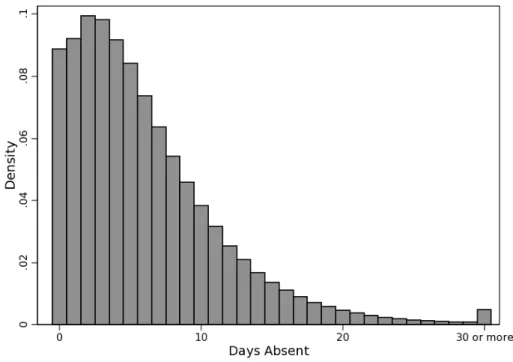
Table 1 presents descriptive information on the sample of students in grades 3 to 5. Students are absent on average 6.13 days of school prior to the exam. Figure 1 depicts the distribution of absences in the data. While the distribution is centered around 5 days of class, a sizable proportion of students are absent for much longer; 25% percent of students miss nine days (just under two weeks) of class and 10% miss 13 days or more prior to the day of the exam in each year. Interpretation of results typically focuses on the effect of the average number of absences on performance. However, it is important to recognize that for a sizable share of the sample, 30More information on North Carolina’s attendance policies can be found at:
reducing absences would have a much larger impact.
North Carolina has an ethnically diverse student body with 25.3% black and over 10% Hispanic. Relative to the United States in the 2010 Census, North Carolina has a greater share of black school-age children and a slightly smaller Hispanic population. Males and females are equally represented in the data. Just under half of elementary school students are eligible for the free or reduced price lunch subsidy program, a measure of low-income status. In addition, 13.98% of students are categorized as special education students and 6.4% are English language learners. Finally the proportion of students that has ever been suspended is 6.64%, where the average number of days suspended is 3.05. Note that North Carolina ranks third nationally in the rate of school suspensions behind South Carolina and Delaware.
Table 1: Descriptive Statistics for North Carolina Public School Students
Mean
s.d.
Days Absent
6.13
5.53
Days of Class
166.30
3.48
Suspensions:
Ever Suspended (%)
6.64
24.89
Days Suspended*
3.05
4.22
Race (%):
White
56.90
49.52
Black
25.32
43.49
Hispanic
10.33
30.44
Asian
2.32
15.04
Other
5.13
22.07
Gender (%):
Male
49.94
50.00
Female
50.06
50.00
Other characteristics (%):
Free/reduced lunch eligible
46.65
49.89
Special education
13.98
34.68
English language learner
6.40
24.48
N
1,001,032
Source: NCERDC, 2006-2010. End of grade test scores are standardized by year and grade level. Samples are based on students having two or more observations with required test scores and total absences information, linked to a teacher with at least 5 and no more than 30 students. Final analytical samples also require non-missing information for all included variables.
*Conditional on suspension.
As younger students are less likely to skip school without parental knowledge, by limiting the
sample of analysis to grades 3 to 5 we are able to minimize issues of endogeneity.31 In addition,
31In the NCERDC data, middle school students do in fact exhibit slightly more absences, driven largely by a greater
students in these grades are more likely to enjoy self-contained classrooms and therefore the link between teachers and students is more reliable as compared to those in higher grades.
Figure 1: Distribution of Absences
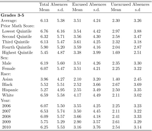
Researchers have demonstrated that students with greater attendance than their classmates perform better on standardized achievement tests and that schools with higher rates of daily attendance tend to generate students who perform better on achievement tests than do schools with lower daily attendance rates [Roby (2004); Sheldon (2007)]. Table 2 examines absences
by student characteristics, including quintile of last year’s prior math score.32 Students with
lower prior year test scores generally have a greater number of absences. This result is largely driven by unexcused absences which exhibits a stronger negative relationship with math test
scores.33 This suggests that students who are less capable are also more likely to miss school.
Simple ordinary least squares (OLS) will therefore result in biased coefficient estimates; without adequate controls, part of any estimated effects of absences will reflect a downward ability bias due to endogenous selection.
Table 2 also highlights racial and gender differences in total number of absences as well as their distribution between excused and unexcused types. White students have a greater number 32
Scores are comparable across time and grades through the use of a developmental scale. The developmental scale is created from the number of correctly answered questions on the standardized test. Each point of the developmental scale measures the same amount of learning. For example, a student who shows identical growth on this scale in two consecutive grades is interpreted as having learned equal amounts in each year.
33
Table 2: Average Number of Absences
Total Absences
Excused Absences
Unexcused Absences
Mean
s.d.
Mean
s.d.
Mean
s.d
Grades 3-5
Average:
6.13
5.38
3.51
4.24
2.30
3.26
Prior Math Score:
Lowest Quintile
6.76
6.16
3.54
4.42
2.97
3.88
Second Quintile
6.32
5.71
3.56
4.30
2.58
3.47
Third Quintile
6.13
5.47
3.61
4.25
2.32
3.18
Fourth Quintile
5.90
5.20
3.59
4.16
2.04
2.87
Highest Quintile
5.45
4.87
3.38
3.99
1.69
2.51
Sex:
Male
6.19
5.60
3.51
4.26
2.35
3.30
Female
6.07
5.47
3.51
4.21
2.25
3.22
Race:
Asian
3.96
4.27
2.10
3.20
1.40
2.45
Black
5.52
5.51
2.52
3.66
2.67
3.69
Hispanic
5.27
4.95
2.55
3.49
2.50
3.35
White
6.59
5.58
4.17
4.49
2.11
3.02
Year:
2006
6.07
5.50
3.55
4.25
2.25
3.23
2007
6.53
5.74
3.50
4.45
2.11
3.22
2008
6.09
5.57
3.66
4.18
2.41
3.33
2009
5.75
5.29
2.90
3.57
2.61
3.29
2010
6.25
5.53
3.16
3.76
2.54
3.14
Source: NCERDC, 2006-2010. Samples are based on students having two or more observations with required test scores and total absences information, linked to a teacher with at least 5 and no more than 30 students. The sum of excused and unexcused absences do not sum to total absences as absence counts by type are only available for about two-thirds of the student-year observations. When missing, absences by type are generally missing at the school, rather than student, level.
of absences than other racial groups with an average of 6.59 days a year. Blacks and Hispanics are absent 5.52 and 5.27 days respectively. However, a greater share of absences are excused for white students relative to both the other two racial groups. Males have slightly more absences than do females due to a greater number of unexcused absences. There does not appear to be any time trend in absences.
Although students may have varying quantities of instructional time prior to end of grade tests resulting from absences, schools also differ in the number of actual class days prior to exam administration. During the sample period, the Department of Education mandated 180 days
of class.34 However, the North Carolina Department of Public Instruction dictates a window
of time for exam administration with the specific testing date chosen by the local education 34Only two districts, Forsyth and Guilford Counties, had additional days of class.
Figure 2: Distribution of Days of Class, 2009-2010
agency (LEA).35 As a result, students at different schools may have had differing number of
instructional days at the time academic performance was measured, as can be seen in Figure 2. While schools are not actually extending the school year, the number of instructional days prior to the test are adjusted when the LEA sets the school’s EOG testing date. This variation in
instructional days,36 coupled with data on absences allows for the separate identification of the
effect of absences from additional days of schooling.37 Since schools with more days prior to
the exam are those that are more interested in making use of the additional class time as North Carolina schools face pressure from both state and federal accountability policies [Aucejo and Romano (2014)], the estimated effects on school days are likely an upper bound once we control
for student and school characteristics.38,39
35
http://www.ncpublicschools.org/accountability/calendars/archive lists the testing windows for all tests adminis-tered in North Carolina since 2001. A LEA in North Carolina is typically a county.
36
The number of days of class prior to the EOG exam varies between 158 and 180 days.
37
The exam date is set at the beginning of the school year. Therefore, schools cannot extend the number of days of class until the day of the exam based on shocks that occur during the academic year.
38
All schools should not be expected to set the same testing date as administering the test later in the year is more costly due to administrative reasons.
39
The fact that the North Carolina Department of Public Instruction dictates a window of time for exam admin-istration leads to some concerns regarding cheating (i.e. schools that take the exam earlier may provide information about the test to schools that take it later). While NC public school system has adopted many measures to avoid this type of behavior, it is difficult to completely rule out this possibility. However, if cheating were driving our results we would expecte large effects on days of class (i.e. taking the exam later), but this is not the case.
4
Methodology
The data enable us to observe the EOG test score, the number of class days, and the absence of students in each year for grades 3 through 5 until the day of the test. Our primary aim is twofold; to estimate the causal effect of both absence and an additional day of instruction on performance. The number of instructional days prior to the exam varies across schools and years and therefore enables the identification of the effect of absences separately from additional instructional time.
In analyzing the effect of absences on performance, there are potential problems of endo-geneity bias. As shown in Table 2, more able and motivated students appear more likely to both attend school and score highly in their courses and on standardized tests. Therefore, without adequate controls part of any estimated effects of absences will reflect a downward bias due to endogenous selection. This bias could be minimized with good proxies for ability,
engagement/motivation, or other individual characteristics.40
Our first strategy to deal with the potential problem of ability bias is to use the panel prop-erties of the data. Student fixed effects are employed to control for all observed and unobserved student characteristics that are constant over time. This potentially includes student effort, motivation and ability, as well as familial factors such as parental willingness for their child to miss school or their efforts to help with school work at home.
School fixed effects are also included in the model to control for the common influences of a school by capturing systematic differences across institutions. This includes curriculum, hiring practices, school neighborhood, and the quality of leadership. These effects are identified by students who switch schools during grades 3 through 5. Teacher fixed effects are included to control for the common influences of a teacher. Finally, fixed effects for grade and year will parse out the effect of schools and teachers from other common influences that occur across the population in a given year and for a given cohort.
The main estimating equation is:
yigkst“β0`β1ait`β2dist`β3Xit`β4Gig`β5Tt`αi`θk`δs`igkst (1)
whereyigkstdenotes the test score of studenti, in gradeg, teacherk, schools, and yeartwhere
the test score is standardized by grade, year and subject. The main explanatory variables of
interest areait anddist;ait is the number of absences over the course of the school year up to
40
The data contains information on the students’ prior year test score which is also included in several specifications of the model.
the day of the exam;dist is the number of days of instruction prior to the examination day. X
is a vector of student covariates,Gare grade fixed effects, andT are time fixed effects. αi, θk,
andδsdenote student, teacher, and school fixed effects respectively.
A value-added model of student achievement is also implemented. The feature of including a lagged achievement score at the individual level means that under the assumptions of the model, it is no longer necessary to incorporate additional measures of ability or a full historical panel of information on any particular student.
Estimating Equation 1 by ordinary least squares solves:
min β,α,θ,δ N ÿ i“1 K ÿ k“1 S ÿ s“1 pyigkst´β0´β1ait´β2dist´β3Xit´β4Gig´β5Tt´αi´θk´δsq2 (2)
Given the large number of students (382,835), teachers (29,202) and schools (1,305) in our data, after using student fixed effects to control for individual heterogeneity, incorporating a dummy variable for each teacher and for each school would be infeasible. We employ an iterative fixed-effects estimator introduced by Arcidiacono, Foster, Goodpaster, and Kinsler (2012) to reduce the computational cost of estimating the multi-level fixed effects model of student achievement. This method yields OLS estimates of the parameters of interest while circumventing the dimensionality problem. The algorithm begins with an initial guess of the
parametersαpi0q, θkp0q, δsp0q. It then iterates on the following steps with themthiteration:
• Step 1: Using the initial guesses of the student, teacher, and school fixed effects, calculate
Zigkstpmq “yigkst´αp mq i ´θ pmq k ´δ pmq
s and solve the least squares problem:
! β01pmq, β11pmq, β21pmq, β13pmq, β41pmq, β51pmq ) “ arg min β N ÿ i“1 K ÿ k“1 S ÿ s“1 pZigkstpmq ´β0´β1ait´β2dist´β3Xit´β4Gig´β5Ttq2 • Step 2: Using ! β01pmq, β11pmq, β21pmq, β31pmq, β41pmq, β51pmq, θkpmq, δpsmq ) calculate αpim`1q based
on the following expression (kPidenotes teachers of studenti)
αpim`1q“ ř kPi pyigkst´β 1pmq 0 ´β 1pmq 1 ait´β 1pmq 2 dist ´β13pmqXit´β 1pmq 4 Gig´β 1pmq 5 Tt´θp mq k ´δ pmq s q ř k IpkPiq
where the previous expression avoids the minimization over all the α1
ex-pression is obtained from the first order condition of the least squares problem with respect to
αi
• Step 3: Using!β01pmq, β11pmq, β21pmq, β31pmq, β41pmq, β51pmq, αpim`1q, δpsmq
)
calculateθpkm`1qin an
analogous way to step 2.
• Step 4: Using!β10pmq, β11pmq, β21pmq, β31pmq, β41pmq, β51pmq, αpim`1q, θkpm`1q)calculateδspm`1q in an analogous way to step 2.
• Step 5: Repeat steps 1 to 4 until convergence of the parameters.
5
Baseline Results
Table 3 presents the regression results for math and reading, based on Equation 1. Specification (1) is a simple OLS regression of standardized test scores without any fixed effects or controls
for student ability.41 The coefficients on absences for both math and reading are negative,
sig-nificant and large in magnitude. However, since there are no controls for unobserved individual characteristics which is likely to be negatively correlated with absences, the coefficient is bi-ased downward; we expect that once adequate controls are included, the coefficient on absences will increase. Similarly, the coefficient on days of class is the opposite sign from what was hypothesized and likely also suffers from omitted variable bias.
Specification (2) includes student fixed effects, thereby controlling for observed and unob-served student characteristics that are constant over time. An additional absence results in math (reading) scores declining by 0.66% (0.35%) of a standard deviation. Therefore, a student
with the average number of absences42 would see their math (reading) score decline by 4.05%
(2.15%) of a standard deviation. Additional days of class has a positive, but insignificant effect on both math and reading performance. The addition of school fixed effects (specification (3))
has little effect to the magnitude of the coefficient of interest for either subject.43
Specification (4), our preferred specification, includes triple fixed effects and finds signifi-cant, although slightly smaller coefficients on days absent relative to the previous specifications. Reducing absences by the average (6.13 days) results in scores declining 3.56% and 1.84% of a standard deviation respectively for math and reading. Additionally, the effect of days of class on math test scores is now significant, although smaller in magnitude relative to absences, with test 41
In addition to the regressors specified in Equation 1, controls for gender and ethnicity are also included.
42The average student in grades 3-5 is absent 6.13 days of school. 43
Table 13 (in the appendix) provides an alternative specification where number of days absent is divided by days of class. Results remain very similar.
T
able
3:
Bas
elin
e
Regression
Math T est Score Readin g T est Score (1) (2) (3) (4) (5) (1) (2) (3) (4) (5) Da ys Absen t -0.0192*** -0.0066*** -0.0065*** -0.0058*** -0.0076*** -0.0104*** -0.0035*** -0.0034*** -0.0030*** -0.0039*** (0.0002) (0.0002) (0.0002) (0.0002) (0.0001) (0.0002) (0.0002) (0.0002) (0.0002) (0. 0001) Da ys of Class -0.0075*** 0.0002 0.0000 0.0008** 0.0011** -0.0056*** 0.0003 0.0001 0.0002 0.0016*** (0.0003) (0.0003) (0.0002) (0.0004) (0.0004) (0.0003) (0.0003) (0.0003) (0.0004) (0. 0004) Studen t FE No Y es Y es Y es No No Y es Y es Y es No Sc ho ol FE No No Y es Y es Y es No No Y es Y es Y es T eac her FE No No No Y es Y es No No No Y es Y es Lagged Studen t Score No No No No Y es No No No No Y es N 1,001,032 1, 001,032 1,001,032 1,000,904 872,860 1,001,032 1,001,032 1,001,032 1,000,904 872,860 Source: NCERDC, 2006-2010, grades 3-5. Dep enden t v ariable is standardized b y grad e and y ear. All sp ecifications include dumm y v ariables fo r grade, y ear, and free/reduced price lunc h status. Sp ecifications without studen t fixed effects also include dumm y v ariables for race and gender. Bo otstra pp ed standard errors are rep orted in pare n thesis. Significanc e lev e ls: ˚ ˚ ˚ denotes 1%; ˚˚ denotes 5%; ˚ denotes 10%.scores increasing 0.49% of a standard deviation for an equivalent increase in school days.
Spec-ifications (5) examines a model with lagged achievement, and teacher and school fixed effects.44
The results are slightly larger in magnitude relative to the preferred specification; reducing ab-sences by the average results in scores declining by 4.66% and 2.39% of a standard deviation for math and reading respectively. The equivalent increase in school days would increase math scores by 0.67% and reading scores by 0.98% of a standard deviation.
In summary, the absolute value of the effect of each additional absence on test scores appears to be larger relative to extra days of class. Additional days of class seem to have a positive effect on math scores, although on reading the effects appear smaller according to specifications 3 and 4. Similarly, Lee and Barro (2001) and Sims (2008) find small or no effect on reading scores. That both absences and additional days of class seem to have a greater effect on math achievement than on reading achievement is consistent with the general finding that educational inputs and policy have relatively larger impact on math achievement [Hanushek and Rivkin (2010); Jacob (2005); Rivkin, Hanushek, and Kain (2005)], perhaps because children are more likely to be exposed to reading and literacy outside of school, particularly at home where parents may be more apt to help their children learn and develop reading skills [Currie and Thomas (2001)].
6
Robustness Checks
Despite the set of controls that have been included in Table 3 (i.e. student, teacher, and school fixed effects, previous year test score and free-reduce price lunch status), our results on absences may still be driven by confounding effects. For example, student engagement may not be fixed over time or family/health shocks could affect absences and test score performance in a way that may not be captured by our extensive set of controls. In this regard, this section provides a series of robustness checks.
6.1
Student Disengagement
The fact that students may lose interest in classroom activities during their schooling career, suggests that the dynamic component of this type of behavior cannot be captured by the addition of student fixed effects. This may cause concern that our results on absences are in fact driven by a correlation between “lack of interest in school” and the decision to not attend class. To this 44
The sample size is smaller in this specification because for a given year we do not have data on previous year test scores for students (except in grade 3). Running a specification with triple fixed effects on this sample provides similar results as the ones currently reported in specification 4 (i.e. the change in the sample size is not driving the difference in results).
end, we present several pieces of evidence that assess the importance of this potential threat to our identification strategy.
First, recall that our sample corresponds to students from grades 3 to 5. Therefore, the decision to be absent from school needs to be (at least tacitly) supported by their parents. This suggests that endogeneity issues should be of a less concern relative to a sample of high school students.
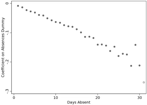
Second, if student disengagement is the main driver of our results, then it is likely to have a nonlinear effect on absences. For example, the effect of being absent 10 days at school during the academic year due to (for instance) disengagement is expected to be disproportionally larger than the effect of being absent just 2 days at school. To explore this, we saturated the variable absences with dummies for each day absent from 1 to 30 and another for 31 or more. The
coefficients on each of the days absent dummies are plotted in Figure 3.45 The pattern of the
coefficients indicates that the effect on test scores is in fact roughly linear through 30 absences. The lack of nonlinear effects suggests that disengagement effects are not likely to be driving our results on absences.
Figure 3: Coefficients on Days Absent Dummy Variables
4645
These coefficients are obtained after controlling for student heterogeneity with standardized math scores as the dependent variable. Results are similar for reading scores.
46
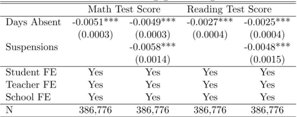
Table 4: Student Disengagement Regression
Math Test Score
Reading Test Score
Days Absent
-0.0051***
-0.0049***
-0.0027***
-0.0025***
(0.0003)
(0.0003)
(0.0004)
(0.0004)
Suspensions
-0.0058***
-0.0048***
(0.0014)
(0.0015)
Student FE
Yes
Yes
Yes
Yes
Teacher FE
Yes
Yes
Yes
Yes
School FE
Yes
Yes
Yes
Yes
N
386,776
386,776
386,776
386,776
Source: NCERDC, 2006-20008, grades 3-5. Dependent variable is standardized by grade and year. All specifications include days of class and dummy variables for grade, year, and free/reduced lunch participation. Bootstrapped standard errors are reported in parenthesis. The sample is smaller than our main estimating sample as suspensions are only available until year 2008 and for approximately two-thirds of the student-year observations. Suspensions are generally missing at the school level. Significance levels: ˚ ˚ ˚denotes 1%;˚˚denotes 5%;˚denotes 10%.
Third, we include a proxy for student disengagement to our baseline specifications. More specifically, a measure of misbehavior, total days suspended, is added. The total days suspended
is the sum of in-school and out-of-school suspensions.47 If student disengagement is affecting our
results, we should expect a large decline in the effect of absences once controlling for suspensions. Table 4 shows that the coefficient on absences are in fact fairly constant across specifications.
The first column for both math and reading corresponds to the baseline specification in Table 3.48
For math (reading), the effect on absences only changes from -0.0051 (-0.0027) in our baseline specification to -0.0049 (-0.0025) after controlling for suspensions (see columns 2 and 4).
Finally, we follow an instrumental variables approach, where we instrument number of ab-sences with data on flu outbreaks at the county level in North Carolina. The flu is a contagious respiratory illness that affects all ages; however, school-aged children are the group with the
highest rates of flu illness.49 In this regard, we make use of data from the North Carolina
Dis-ease Event Tracking and Epidemiolgic Collection Tool (NC DETECT) provided by the North
Carolina Division of Public Health50 which has been collecting the number of influenza-like
47
In-school suspensions are usually served in an in-school suspension classroom. When a school does not have an in-school suspension program or when offenses are more serious or chronic, they may be dealt with through short-term, out-of-school suspensions. Long-term suspensions are more than ten days in length may be used for more serious offenses and are served out-of-school. Approximately 6.6% of our sample has been suspended at some point in time.
48
The sample size is smaller as not all schools report suspensions (around one third of the sample), and data on suspensions is only reported for approximately 1% of the sample after 2008; as a result, we exclude those years.
49
Center for Disease Control, http://www.cdc.gov/flu/school/guidance.htm
50
NC DETECT is an advanced, statewide public health surveillance system. NC DETECT is funded with fed-eral funds by North Carolina Division of Public Health (NC DPH), Public Health Emergency Preparedness Grant (PHEP), and managed through a collaboration between NC DPH and the University of North Carolina at Chapel Hill Department of Emergency Medicine’s Carolina Center for Health Informatics (UNC CCHI).
illnesses (ILI) affecting kids between the age of 5 and 12 years since January of 2008.51,52
In order for a measure of flu activity to be an appropriate instrument for absences, it must be correlated with absences and only impact test score performance through missing days of schooling. While one may be concerned that the flu has a direct impact on EOG scores, the
flu season commonly peaks in January, February, or March53 well before the EOG tests are
administered.54 Moreover, our data shows low flu activity during the months exams take place.55
Therefore, this is not likely to be an important threat to our identification strategy. However, even though our data corresponds to flu cases in children between the ages of 5 and 12, a possible concern is that flu outbreaks may also affect teacher attendance, and therefore may confound the effects of student and teacher absences. Unfortunately, we only have data on teacher absences due to sickness through the 2008 school year, while our data on flu outbreaks starts in January of 2008. However, as we show in the appendix (Table 15), adding teacher sick days to our baseline
specification does not affect our coefficient on either days absent or school days.56 Furthermore,
it does not have a substantial effect on students performance. This result is consistent with the fact that the availability of substitute teachers in North Carolina is likely to lessen the potential harm from teacher absences.
We define the instrument as:
IVf lu,c,yr“ ¨ ˝ ř m ILIc,m Nc,yr 10,000 ˛ ‚
whereILIc,m is the number of influenza-like illness cases in countyc in monthm(the analysis
only uses data from August to June, which corresponds to the academic year) and Nc,yr is
51
ILI cases are reported by N.C. hospital emergency departments.
52More specifically, NC DETECT has provided the total number of ILI cases per month in each N.C. county
affecting kids between the age 5 to 12 (the total number of counties in N.C. is 100). If the number of cases in a given county-month data cell is greater than 0 but less than 10, then the information is censored. We use multiple imputation techniques [Royston (2007)] in order to deal with those values that we do not observe but we know are in the range between 1 and 9 visits. Table 14 (in the appendix) shows that results are similar if instead of using multiple imputation techniques, we just replace the censored values with specific numbers (i.e. 1, 5, or 9). Finally, we aggregate the data at the academic year level (i.e. August to June); the resulting proportion of ILI cases that are imputed is small (i.e. 7.9% across both the 2008/09 and 2009/10 seasons).
53
According to CDC, in the last thirty years flu activity most often peaked in February (45% of the time), followed by December, January and March (which each peaked 16% of the time). It has never peaked after March. Source: http://www.cdc.gov/flu/about/season/flu-season.htm
54EOG tests are generally administered at the end of May or later. The inclusion of controls for ILI activity in
May and June in our baseline regressions do not alter the results.
556.3% of yearly flu visits occurred in May and 5.8% in June. 56
The results do not change across specifications (with or without teacher sick days) but the coefficient on school days becomes insignificant due to the fewer number of years that we can use in this regression (i.e. only years 2006-2008), therefore leading to less variability over time.
number of students in elementary school in county c during the academic year yr.57 The IV
then is the number of ILI cases per 10,000 school-aged children.58
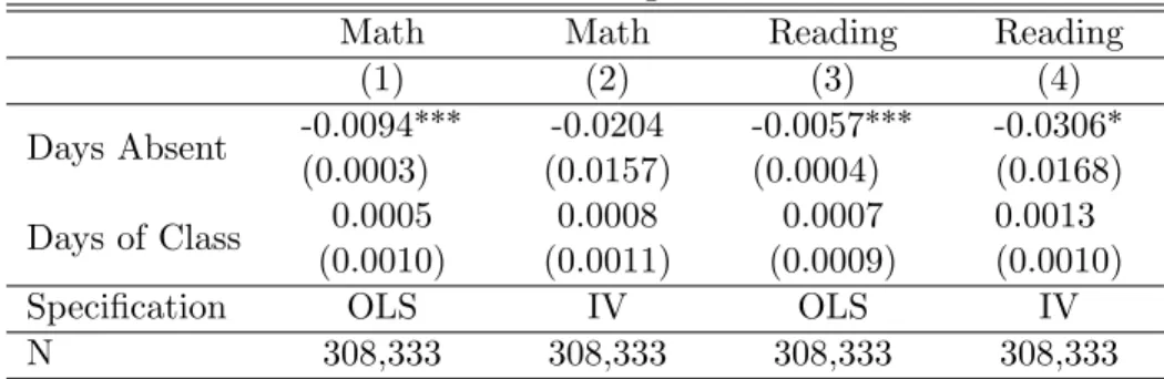
Table 5 shows the results of OLS (benchmark case) and IV regression specifications for math
and reading.59 Columns (2) and (4) indicate that the effect of absences after instrumenting
with flu outbreaks is larger than days of class.60,61However, the IV specifications indicate that
a one day reduction in excused absences would lead to increases of 2.0% and 3.1% of a standard deviation in math and reading respectively. This is approximately twice our benchmark OLS
specification results for math, and a five-fold increase for reading.62
To sum up, the linearity in the effect of absences, in addition to the fact that including suspensions and instrumenting absences with flu data are not affecting our main results (i.e. larger effect of absences than days of class) suggest that disengagement effects are not likely to be driving our results.
Table 5: IV Regression
Math
Math
Reading
Reading
(1)
(2)
(3)
(4)
Days Absent
-0.0094
˚˚˚(0.0003)
-0.0204
(0.0157)
-0.0057
˚˚˚(0.0004)
-0.0306
˚(0.0168)
Days of Class
0.0005
(0.0010)
0.0008
(0.0011)
0.0007
(0.0009)
0.0013
(0.0010)
Specification
OLS
IV
OLS
IV
N
308,333
308,333
308,333
308,333
Source: NCERDC, 2009-2010, grades 3-5. Dependent variable is standardized by grade and year. All specifications include lagged test score and dummy variables for grade, year, gender, race, and free/reduced-price lunch status. Notice that the sample size is smaller because we only have flu data for the years 2009-2010. Columns (1) and (3) show OLS results (serving as a benchmark case), while columns (2) and (4) show the IV regression results. Bootstrapped standard errors clustered at the school level are reported in parenthesis. Significance levels: ˚ ˚ ˚ denotes 1%;˚˚denotes 5%;˚denotes 10%.
57
The number of students in elementary school in a county is the sum of all students in grades K through 8, which generally corresponds to ages 5-12.
58
The IV variable is defined per 10,000 school-aged children to be consistent with the rest of the literature which typically defines ILI rates per 10,000 or 100,000 population.
59All 2SLS specifications in this paper have very strong first stages (see Table 16 in the appendix). The coefficient
on the instrument has a p-value of 0.000 in all specifications. Figure 4 (in the appendix) shows the presence of substantial variability in the number of flu cases across counties.
60
Though, the math coefficient is (marginally) not statistically significant.
61The exam date is set at the beginning of the school year. Therefore, schools cannot extend the number of
instructional days prior to the exam in response to a severe flu season.
62
Given that IV recovers LATE effects, it is not surprising that the magnitude of the coefficients is larger than in the OLS specifications.
Table 6: Siblings Fixed Effects Regression
Math Score
Reading Score
Days Absent
-0.0072***
-0.0024***
(0.0008)
(0.0008)
Sibling Year FE
Yes
Yes
Lagged Student Score
Yes
Yes
N
86,660
86,660
Source: NCERDC, 2006-2010, grades 3-5. Dependent variable is standardized by grade and year. All specifications include dummy variables for grade. Standard errors are reported in parenthesis. The sample is smaller than our main estimating sample as identification relies on observing at least two children from the same family in a given year. Significance levels: ˚ ˚ ˚denotes 1%;˚˚denotes 5%;˚denotes 10%.
6.2
Family Shocks
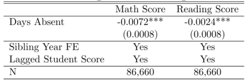
Our baseline specifications thus far have been assuming that family shocks/inputs that are correlated with absences and affect performance are constant across time and therefore taken care of with the inclusion of student fixed effects. However, these estimates may still be biased if there are potentially time varying unobserved family factors that may be influencing both student absences and testing performance. As mentioned previously, we follow Caetano and Macartney (2013) in utilizing the geocoded address data to construct a family ID variable. Table 6 incorporates a family-year fixed effect, which captures all observed and unobserved characteristics that are common to a family-year and is identified off of different incidence of
absences within that year for a family.63 Lagged test score is incorporated in the specification
as a proxy for ability as that is likely to be different even across siblings. The family-year fixed effects specification controls for any family shock, such as parental divorce or a death in the family, that impacted both absences and test scores. Since siblings attend the same school, the coefficient on days of class cannot be well identified. The coefficient on absences in Table 6 indicates that an additional absence decreases scores by 0.72% and 0.24% for math and reading respectively, which is similar to our previous findings. This suggests that family specific shocks are not driving the results.
63
The information in the data does not provide the biological relationship between children living in the same household. Regardless, since the students are residing in the same household and are therefore exposed to shared family characteristics, children living at the same address will be considered family. There are 31,856 sibling groups that are observed in grades 3-5 in the same year. For those sibling groups of size two (over 95% of the siblings sample) observed in the same year, the mean absolute value of the difference in days absent is 2.88 days, with a standard deviation of 3.35 days.
6.3
Health Shocks
Even after all of the controls to guard against endogeneity concerns, fixed effects do not guard against absences that are, for example, the result of a major/chronic illness; which is an excused absence and might be expected to have a direct effect on test scores. If this was driving our results, then after disaggregating absences into the two types, excused absences would be
ex-pected to be more negative relative to unexcused absences.64 Specification (1) of Table 7 is our
preferred specification from Table 3.65 Specifications (2) and (3) examine the effect of absences
and days of class independently of the other; there is little difference in the magnitude of the effects when comparing to specification (1). The final two columns utilize the sample for which
absences disaggregated by types are available.66 For comparison purposes, specification (4) is
the same as specification (1) but with the sample of students for which there are data on absences disaggregated by type. The results are similar for both absences and days of class. Specification (5) presents results disaggregating absences by type. An additional excused absence lowers math (reading) scores by 0.43% (0.22%) of a standard deviation, while unexcused absences have an effect of 0.74% (0.46%) of a standard deviation. Therefore, these results indicate that health problems do not seem to bias our results.
The evidence presented in this section indicates that our baseline findings on the effect of students’ absences on test scores performance are robust to several specifications, suggesting that possible expected threats to our identification strategy are not driving the results.
7
Heterogeneous Effects
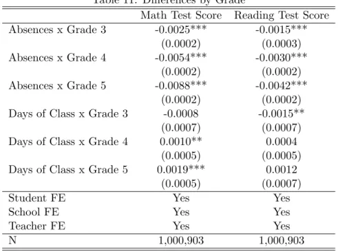
On average, absences have a negative effect on test scores, while the positive impact of an additional day of class within the observed range is much smaller. However, these effects may differ based on student characteristics. As noted earlier, catching up after an absence is likely to be more difficult for a low performing student. Understanding the heterogeneous effects of an absence will help to inform the policy discussion by identifying groups of the population that are likely to disproportionately benefit from particular interventions.
To examine how the effect of attending school differs by student ability, students are grouped based on their test score from the prior year. Table 8 shows the regression results with absences 64Gottfried (2009) also examines disaggregated absences and finds that students with a higher proportion of
unex-cused absences places them at academic risk, particularly in math achievement.
65Specifications (1)-(3) only use years 2006-2008 as those are the years in which we have absences by type
infor-mation.
66As mentioned previously, absences by type are not available for the full sample. They are generally missing at
T
able
7:
Absences
b
y
T
yp
e
Regression
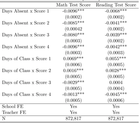
Math T est Score Reading T est Score (1) (2) (3) (4) (5) (1) (2) (3) (4) (5) Da ys of Class -0.0005 -0.0008 -0.0005 -0. 0006 0.0005 0.0003 0.0004 0.0004 (0.0009) (0.0009) (0.0009) (0.0009) (0.0008) (0.0008) (0.0009) (0.0009) Da ys Absen t -0.0055*** -0.0055*** -0.0056*** -0.0031*** -0.0031*** -0.0031*** (0.0002) (0.0002) (0.0002) (0.0002) (0.0002) (0.0002) Excused Absences -0.0043*** -0.0022*** (0.0003) (0.0002) Unexcused Absences -0.0074*** -0.0046*** (0.0004) (0.0004) Studen t FE Y es Y e s Y es Y es Y es Y es Y es Y es Y es Y es Sc ho ol FE Y e s Y es Y es Y es Y es Y es Y es Y e s Y es Y es T eac her FE Y es Y es Y es Y es Y es Y es Y es Y es Y es Y es N 509,890 509,890 509,890 486,694 486,694 509,890 509,890 509,890 486,694 486,694 Source: NCERDC, 2006-2008, grades 3-5. Dep enden t v ariable is standardized b y grad e and y ear. All sp ecifications include dumm y v ariables fo r grade, y ear, and free/reduced price lunc h status. Bo otstrapp ed standard errors are rep orted in paren thesis. Significance lev els: ˚ ˚ ˚ denotes 1%; ˚˚ denotes 5%; ˚ denotes 10%.and days of class interacted with a dummy for the quartile of the prior year’s score. Score 1 denotes the lowest quartile and score 4 the highest. These results indicate that students in the
lowest quartile are most adversely affected by an additional absence in both math67and reading;
consistent with the hypothesis that lower ability students have a harder time making up missed work. A similar pattern can be found when considering days of class, i.e. low achieving students benefit the most from spending more time at school. Results also show the same pattern as before when comparing the effect of an absence relative to an extra day of class within achievement level. Namely, absences have larger effects than days of class. In order to provide a robustness check, given that just controlling for quartiles of previous year achievement may not be enough to account for student heterogeneity, Table 9 estimates Equation 1 with absences and days of class interacted with student fixed effects. The estimation outcomes show that the effects of both absences and additional days of class are muted for higher ability students which is consistent with our earlier results. For example, the effect of an absence in math (reading) performance for
a student in the 25th percentile of the student fixed effect distribution68is 18.6% (69.4%) larger
than for a student in the 75th percentile. To sum up, the findings in Tables 8 and 9 suggest that policies aiming to extend time spent at school (either through reducing absences or extending the school calendar) are likely to have larger impact on low achieving students, helping to close current gaps in performance.
Table 10 further explores the relationship between absences and the quality of students, teachers, and schools by regressing days absent on the three fixed effects from our preferred
specification of the baseline regression (specification (4) in Table 3).69 As expected from our
previous results, lower ability students have more absences than their higher ability peers. However, we also find that worse schools (teachers) have a positive relationship with absences. More specifically, an increase in school (teacher) quality from the 25th percentile to the 75th
percentile is associated with 0.14 (0.13) fewer days absent.70 This is a relatively large effect given
the sample average of 6.13 absences. In this regard, improving the quality of schools and teachers could not only benefit students by providing them with a better educational environment, but 67
The lowest quartile interacted with absences is significantly different from the middle two quartiles. The top of the distribution has similarly negative effects on math scores. The highest quartile is not significantly different from the lowest quartile, but is from the others. Notice that this specification is controlling for quartile of previous year test score performance, instead of using a continuous measure of performance as in Table 3.
68
The 25th and 75th percentile of the math (reading) student fixed effect distribution are -0.937 (-0.997) and 0.996 (1.108), respectively.
69Given that the fixed effects from the math and reading regressions are different, we present two set of results (i.e.
the first column includes fixed effects from the math specification while the second column includes the fixed effects from the reading specification).
70
This result corresponds to the specification that includes the fixed effects obtained from the regressions that use as dependent variable math test score.