3-2018
Using the multivariate spatio-temporal Bayesian
model to analyze traffic crashes by severity
Chenhui Liu
Iowa State University, [email protected] Anuj Sharma
Iowa State University, [email protected]
Follow this and additional works at:https://lib.dr.iastate.edu/ccee_pubs
Part of theCivil Engineering Commons,Multivariate Analysis Commons, and the Transportation Engineering Commons
The complete bibliographic information for this item can be found athttps://lib.dr.iastate.edu/ ccee_pubs/179. For information on how to cite this item, please visithttp://lib.dr.iastate.edu/ howtocite.html.
This Article is brought to you for free and open access by the Civil, Construction and Environmental Engineering at Iowa State University Digital Repository. It has been accepted for inclusion in Civil, Construction and Environmental Engineering Publications by an authorized administrator of Iowa State University Digital Repository. For more information, please [email protected].
crashes by severity
AbstractUnobserved heterogeneity across space, time, and crash type is often non-negligible in crash frequency modeling. When multiple crash types with spatial and temporal features are analyzed, multivariate spatio-temporal models should be considered. For this study, we analyzed the yearly county-level fatal, major injury, and minor injury crashes in Iowa from 2006 to 2015 using a multivariate spatio-temporal Bayesian model. The model adopted a multivariate spatial structure, a multivariate temporal structure, and a multivariate spatio-temporal interaction structure to account for possible correlations across injury severities over space, time, and spatio-temporal interaction, respectively. Income and weather indicators were found to have no significant effects on crash frequencies in the presence of vehicle miles traveled and unemployment rate. Both spatial and temporal effects were found to be important, and they played nearly the same roles for all three crash types in the studied dataset. Counties located in north and southwest Iowa were found to tend to have fewer crashes than the remaining counties. All three crash types generally showed descending trends from 2006 to 2015. They also had significantly positive correlations between each other in space but not in time. The crude crash rates and predicted crash rates were generally consistent for major injury and minor injury crashes but not for low-count fatal crashes. High-risk counties were identified using the posterior expected rank by the predicted crash cost rate, which was more able to truly represent the underlying traffic safety status than the rank by the crude crash cost rate.
Keywords
Multivariate spatio-temporal, Bayesian, Crash frequency, Posterior expected rank, Crash cost rate Disciplines
Civil Engineering | Multivariate Analysis | Transportation Engineering Comments
This is a manuscript of an article published as Liu, Chenhui, and Anuj Sharma. "Using the multivariate spatio-temporal Bayesian model to analyze traffic crashes by severity."Analytic Methods in Accident Research17 (2018): 14-31. DOI:10.1016/j.amar.2018.02.001. Posted with permission.
Creative Commons License
This work is licensed under aCreative Commons Attribution-Noncommercial-No Derivative Works 4.0 License.
Using the Multivariate Spatio-Temporal Bayesian Model to
Analyze Traffic Crashes by Severity
Chenhui Liuab*, Anuj Sharmaa
aDepartment of Civil, Construction, and Environmental Engineering, Iowa State University.
InTrans, 2711 South Loop Drive, Suite 4700, Ames, IA 50010-8664
bDepartment of Statistics, Iowa State University
* Corresponding author
Email addresses: [email protected] (C. Liu), [email protected] (A. Sharma)
Abstract
Unobserved heterogeneity across space, time, and crash type is often non-negligible in crash frequency modeling. When multiple crash types with spatial and temporal features are analyzed, multivariate spatio-temporal models should be considered. For this study, we analyzed the yearly county-level fatal, major injury, and minor injury crashes in Iowa from 2006 to 2015 using a multivariate spatio-temporal Bayesian model. The model adopted a multivariate spatial structure, a multivariate temporal structure, and a multivariate spatio-temporal interaction structure to account for possible correlations across injury severities over space, time, and spatio-temporal interaction, respectively. Income and weather indicators were found to have no significant effects on crash frequencies in the presence of vehicle miles traveled and unemployment rate. Both spatial and temporal effects were found to be important, and they played nearly the same roles for all three crash types in the studied dataset. Counties located in north and southwest Iowa were found to tend to have fewer crashes than the remaining counties. All three crash types generally showed descending trends from 2006 to 2015. They also had significantly positive correlations between each other in space but not in time. The crude crash rates and predicted crash rates were generally consistent for major injury and minor injury crashes but not for low-count fatal crashes. High-risk counties were identified using the posterior expected rank by the predicted crash cost rate, which was more able to truly represent the underlying traffic safety status than the rank by the crude crash cost rate.
Keywords: multivariate spatio-temporal, Bayesian, crash frequency, posterior expected rank
1 Introduction
Traffic crashes have been one of the major sources of fatalities and injuries in the United States. Crash frequency analysis is often used to identify key factors influencing the propensity of crashes, which is important for policymakers as they propose interventions to prevent road traffic crashes. However, unobserved heterogeneity is often an issue in crash frequency modeling, because many crash-related elements are often unavailable. Neglecting unobserved heterogeneity may produce biased and inefficient results (Mannering et al., 2016).
Unobserved heterogeneity may come from many sources. Crashes are usually classified into multiple types by different criteria, and their underlying correlations may produce some unobserved heterogeneity across observations when they are analyzed simultaneously (Mannering and Bhat, 2014; Mannering et al., 2016). Thus, multivariate models, such as the multivariate Poisson log-normal (MVPLN) model, are often adopted (Ma et al., 2008; El-Basyouny and Sayed, 2009; Aguero-Valverde and Jovanis, 2010; El-Basyouny et al., 2014; Zhao et al., 2017). In addition, crash frequency data are always aggregated over space and time, which may also produce unobserved heterogeneity, as crashes that occur close in space or time are very likely to share some unobserved characteristics (Lord et al., 2005; Lord and Mannering, 2010; Savolainen et al., 2011; Mannering and Bhat, 2014; Mannering et al., 2016). Previous studies have shown that spatial correlations of traffic crashes may exist across states/provinces (Erdogan, 2009; Truong et al., 2016), counties (Aguero-Valverde and Jovanis, 2006; Song et al., 2006; Eckley and Curtin, 2013), census tracts (Wang and Kockelman, 2013), traffic analysis zones (Matkan and Mohaymany, 2013), intersections (Ahmed and Abdel-Aty, 2015; Liu et al., 2015) and segments (Aguero-Valverde and Jovanis, 2008; Wang et al., 2009, 2011; Aguero-(Aguero-Valverde, 2011; Jiang et al., 2014; Zeng and Huang, 2014). The similarity of economy, culture, land use, weather, traffic laws, and driving behavior within a given region may explain the spatial correlations in traffic crashes. When multiple crash types with spatial correlations need to be analyzed, multivariate spatial models have been proved to be more powerful than univariate spatial models, as multivariate spatial models can account for correlations across crash types in space in addition to spatial correlations (Miaou and Song, 2005; Song et al., 2006; Valverde, 2013; Wang and Kockelman, 2013; Aguero-Valverde et al., 2016; Barua et al., 2016). Temporal correlations of traffic crashes may exist across year (Wang and Abdel-Aty, 2006; Brijs et al., 2008; Andrey, 2010; Wang et al., 2011; Yannis et al., 2011; Matkan and Mohaymany, 2013; El-Basyouny et al., 2014), month (Quddus, 2008a; Hu et al., 2013), week (Kilamanua et al., 2011; Sukhai et al., 2011; Liu et al., 2015), and day (Brijs et al., 2008). Temporal correlations occur because many traffic-related factors, such as driver behavior, economy, weather, environment, law, and travel demand, often exhibit some temporal features. Similarly, when multiple crash types with temporal correlations need to be analyzed, multivariate temporal models should be considered, as they can account for correlations across crash types in time in addition to temporal correlations (Serhiyenko et al., 2014; Michalaki et al., 2016).
Crashes often have both spatial and temporal features. When only one crash type is analyzed, the univariate spatio-temporal modeling has been proved in some studies to be superior (Miaou et al., 2003; Aguero-Valverde and Jovanis, 2006; Truong et al., 2016; Liu and Sharma, 2017). When multiple crash types need to be analyzed, a multivariate spatio-temporal model may be needed. Ma et al. (2017) used the bivariate spatio-temporal model to analyze the daily non-injury and injury crash rates on 100 roadway segments of I70 in one year at the micro level, and Boulieri et al. (2017) used the bivariate spatio-temporal model to analyze the yearly low severity and high severity accidents of 7932 electoral wards in England from 2005-2013 considering only vehicle miles traveled (VMT). Both studies showed the superiority of the bivariate spatio-temporal model to the univariate spatio-temporal model in terms of goodness of fit.
In this study, we used the multivariate spatio-temporal Bayesian model to analyze the yearly county-level fatal, major injury, and minor injury crash frequencies in Iowa. The goal of this study was to accurately identify the long-term effects of economy and weather on crash frequency in Iowa and to explore the spatial and temporal correlations of crashes. Additionally, the counties were ranked to identify high-risk areas for safety improvement programs, as funding available for safety improvements are often limited and proper ranking can significantly influence the appropriate distribution of safety funding toward areas with more critical needs. Raw crash data-based ranking is easy to use but crude and inefficient (Miaou and Song, 2005). In Bayesian cases, one statistical ranking method is the posterior expected rank (PER), i.e. the posterior mean of the rank by ranking indicators (Miaou and Song, 2005). When rankings are the main interest, the PER method is recommended (Shen and Louis, 1998). The most common ranking indicator is crash rate, but crash rate considering crash cost by injury severity, called the “crash cost rate” in the following analysis, is strongly recommended when injury severity and associated costs are the main concerns (Miaou and Song, 2005). Thus, the PER of the crash cost rate would be used to rank the studied areas based on the predicted results of the multivariate spatio-temporal Bayesian model in this study.
2 Data Description
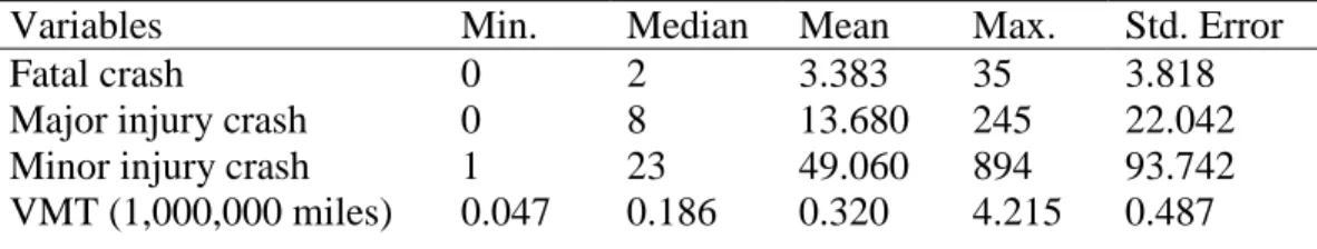
Traffic crash data from Iowa’s 99 counties from 2006 to 2015 were obtained from the Iowa Department of Transportation. Crashes were divided into five categories by severity: fatal, major injury, minor injury, possible injury/unknown, and property damage only. Fatal crashes, major injury crashes, and minor injury crashes were analyzed in this study, as these three types of crashes often lead to significant economic loss and casualties. VMT data for each county in each year from 2006 to 2015 were downloaded from the website of the Iowa Department of Transportation (2016). In addition, unemployment rate data were downloaded from the website of Iowa Community Indicators Program (2016), and per capita personal income data were downloaded from the website of the U.S. Bureau of Economic Analysis (2016) of the U.S. Department of Commerce. Meanwhile, weather data regarding rainfall, snowfall, and the number of days with minimum temperature exceeding 32°F (TH32) were downloaded from the website of the Iowa Environmental Mesonet (2017). These weather data are collected based on the daily climate observations from the National Weather Service’s Cooperative Observer Program. A summary of the variables is given in Table 1. All three crash types have over-dispersion, as their variances are much larger than their means. Additionally, the highest correlation among the covariates was -0.338 (between snowfall and TH32). Thus, no explanatory variables showed strong positive or negative correlations.
Table 1 Descriptive statistics of collected variables
Variables Min. Median Mean Max. Std. Error
Fatal crash 0 2 3.383 35 3.818
Major injury crash 0 8 13.680 245 22.042 Minor injury crash 1 23 49.060 894 93.742 VMT (1,000,000 miles) 0.047 0.186 0.320 4.215 0.487
Unemployment rate (%) 2.000 4.600 4.846 10.200 1.347 Income ($10,000) 2.247 3.877 3.877 6.464 0.666 Rainfall (inch) 17.850 38.610 38.390 64.990 8.570 Snowfall (inch) 0 35 34.560 85.100 14.377 TH32 (days) 174 221 222.600 272 15.733
Note: VMT, vehicle miles traveled; TH32, number of days with minimum temperature exceeding 32°F.
The Pearson correlation coefficients of fatal, major injury, and minor injury crashes were shown in Table 2. All three crash types were highly positively correlated. That is, locations where many fatal/major injury/minor injury crashes were observed likely also had many crashes of the other two types.
Table 2 Pearson correlation coefficients of crash counts
Pearson correlation coefficient Fatal crash Major injury crash Major injury crash 0.837
Minor injury crash 0.835 0.971
The county-level yearly average fatal, major injury, and minor injury crash counts in Iowa are shown in Figure 1. A cluster of high fatal crash frequencies can be observed in the central counties around the dark red-shaded area, where the largest city in Iowa, Des Moines, is located. A cluster of low crash frequencies can be observed in the northern and southwestern regions of Iowa (lightly shaded areas). A cluster of comparatively higher numbers of major injury crashes can also be observed in the central counties. However, no obvious clustering trends can be observed for minor injury crashes. Next, spatial correlations of crashes are examined statistically.
Figure 1 County-level yearly average fatal, major injury, and minor injury crash counts (2006– 2015)
Moran’s I statistic is commonly used to test spatial correlations in traffic crash analyses (Quddus, 2008b; Guo et al., 2010; Xie et al., 2014; Zeng and Huang, 2014). The global Moran’s I is defined as (Anselin, 1988):
𝐼𝐼 =𝑛𝑛 ∑ ∑ 𝜔𝜔𝑖𝑖 𝑖𝑖 𝑖𝑖𝑖𝑖(𝑦𝑦𝑖𝑖−𝑦𝑦�)�𝑦𝑦𝑖𝑖−𝑦𝑦��
∑𝑖𝑖≠𝑖𝑖𝜔𝜔𝑖𝑖𝑖𝑖∑𝑖𝑖(𝑦𝑦𝑖𝑖−𝑦𝑦�)2 (1)
where n is the total number of observations; 𝑦𝑦𝑖𝑖 and 𝑦𝑦𝑗𝑗 are the values of observation 𝑖𝑖 and observation 𝑗𝑗, respectively; 𝑦𝑦� is the average value of observations; and 𝜔𝜔𝑖𝑖𝑗𝑗 is the spatial weight between observations 𝑖𝑖 and 𝑗𝑗.
Negative Moran’s I values indicate negative spatial autocorrelation, positive Moran’s I values indicate positive spatial autocorrelation, and zero indicates no spatial autocorrelation. The z-score of Moran’s I shows if the spatial autocorrelation is significant.
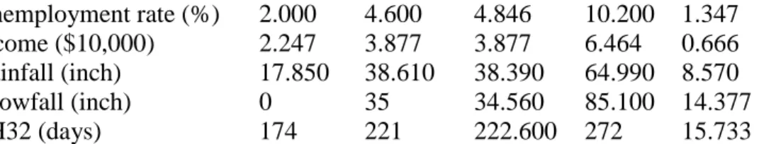
The global Moran’s I statistics of crashes in each year from 2006 to 2015 were calculated using the “spdep” package (Bivand and Piras, 2015) in the R platform (R Core Team, 2016) with queen contiguity spatial weights, where counties with a shared border or vertex were considered neighbors. When areas were neighbors, the spatial weights were 1; otherwise, they were 0. The results are shown in Table 3.
Table 3 Global Moran's I statistics of crash counts in each year
Year
Fatal crash Major injury crash Minor injury crash Standardized Moran's I p-value Standardized Moran's I P-value Standardized Moran's I p-value 2006 1.986 0.024* 1.752 0.041* 0.971 0.166 2007 2.091 0.018* 1.555 0.060 1.141 0.127 2008 1.520 0.064 0.688 0.246 0.871 0.192 2009 1.661 0.048* 1.181 0.119 0.764 0.222 2010 2.486 0.006* 1.586 0.056 1.106 0.134 2011 1.919 0.027* 1.883 0.031* 1.101 0.136 2012 1.240 0.108 2.017 0.022* 1.108 0.134 2013 2.387 0.009* 2.218 0.013* 1.555 0.060 2014 1.241 0.107 1.877 0.030* 1.252 0.105 2015 2.300 0.011* 2.770 0.003* 1.468 0.071 Note: * significant at p = 0.05.
Fatal crash and major injury crash counts showed significant spatial autocorrelations in seven and six out of 10 years, respectively, at a 95% confidence level, but minor injury crash counts did not show any significant spatial autocorrelations at a 95% confidence level in any year. Additionally, the p-values of fatal crash and major injury crash counts were much smaller than those for minor injury crashes. Thus, fatal crashes and major injury crashes were highly likely to be spatially correlated compared to minor injury crashes. These trends may be site specific. As an example, Aguero-Valverde and Jovanis (2006) found injury crash frequencies to have a significant spatial correlation and fatal crash frequencies to not be significantly correlated in counties of Pennsylvania. Although minor injury crash frequencies did not show significant spatial autocorrelations, it does not mean the absence of spatial autocorrelation for minor injury crashes; they may still have weak spatial correlations. The different strengths of spatial autocorrelations imply that the three crash types may have different spatial model parameters.
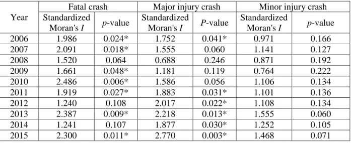
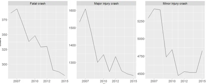
Temporal correlation was not directly tested, as there were only 10 time points for each crash type. However, as shown in Figure 2 by the yearly state-level counts of all three crash types from 2006 to 2015, they all generally exhibited descending trends, with some dipping and heaving and different descending rates.
Figure 2 Iowa state-level yearly crash counts (2006-2015)
3
Methodology
3.1 Statistical Framework
The statistical framework used a Bayesian hierarchical architecture, including both spatial and temporal as well as spatio-temporal interaction components. The statistical model is presented in equations (2) and (3) (Ma et al., 2017):
𝑦𝑦𝑠𝑠𝑠𝑠𝑠𝑠~𝑃𝑃𝑃𝑃𝑖𝑖𝑃𝑃𝑃𝑃𝑃𝑃𝑃𝑃(𝜆𝜆𝑠𝑠𝑠𝑠𝑠𝑠) (2)
log(𝜆𝜆𝑠𝑠𝑠𝑠𝑠𝑠) =𝛼𝛼𝑠𝑠+ 𝑋𝑋𝑠𝑠𝑠𝑠𝑇𝑇∗ 𝛽𝛽𝑠𝑠+υ𝑠𝑠𝑠𝑠+ 𝜈𝜈𝑠𝑠𝑠𝑠+𝜑𝜑𝑠𝑠𝑠𝑠 +𝜃𝜃𝑠𝑠𝑠𝑠 +𝜂𝜂𝑠𝑠𝑠𝑠𝑠𝑠 (3)
where 𝑃𝑃 is the space number, i.e. county number in this case, 1, 2, …, 99; 𝑡𝑡 is the time point, i.e. year number in this case, 1 (2006), 2 (2007), …, 10 (2015); 𝑘𝑘 is the crash injury severity number, 1 (fatal crash), 2 (major injury crash), 3 (minor injury crash); 𝑦𝑦𝑠𝑠𝑠𝑠𝑠𝑠 is the crash count of injury severity 𝑘𝑘 of space 𝑃𝑃 in time 𝑡𝑡; 𝜆𝜆𝑠𝑠𝑠𝑠𝑠𝑠 is the mean crash frequency of injury severity 𝑘𝑘 of space 𝑃𝑃 in time 𝑡𝑡; 𝛼𝛼𝑠𝑠 is the intercept term of crash type 𝑘𝑘; 𝛽𝛽𝑠𝑠 = (𝛽𝛽𝑠𝑠1,𝛽𝛽𝑠𝑠2, … ,𝛽𝛽𝑠𝑠𝑘𝑘) is the m-dimensional regression coefficient vector of crash type 𝑘𝑘 and 𝑚𝑚 is the number of covariates; 𝑋𝑋𝑠𝑠𝑠𝑠 =
(𝑋𝑋𝑠𝑠𝑠𝑠1,𝑋𝑋𝑠𝑠𝑠𝑠2, … ,𝑋𝑋𝑠𝑠𝑠𝑠𝑘𝑘) is the m-dimensional covariate vector of space 𝑃𝑃 in time 𝑡𝑡; υ𝑠𝑠𝑠𝑠 is the structured spatial random effect of crash type 𝑘𝑘 in space 𝑃𝑃; 𝜈𝜈𝑠𝑠𝑠𝑠 is the unstructured spatial random effect of crash type 𝑘𝑘 in space 𝑃𝑃; 𝜃𝜃𝑠𝑠𝑠𝑠 is the structured temporal random effect of crash type 𝑘𝑘 in time 𝑡𝑡; 𝜙𝜙𝑠𝑠𝑠𝑠 is the unstructured temporal random effect of crash type 𝑘𝑘 in time 𝑡𝑡; and 𝜂𝜂𝑠𝑠𝑠𝑠𝑠𝑠 is the spatio-temporal interaction effect of crash type 𝑘𝑘 in space 𝑃𝑃 and time 𝑡𝑡.
The spatial component of each observation consisted of two parts: υ𝑠𝑠𝑠𝑠+ 𝜈𝜈𝑠𝑠𝑠𝑠, and the temporal component also consisted of two parts: 𝜑𝜑𝑠𝑠𝑠𝑠 +𝜃𝜃𝑠𝑠𝑠𝑠.
3.1.1 Spatial Component
3.1.1.1 Univariate Spatial Model
The spatial component of each observation, υ𝑠𝑠𝑠𝑠+ 𝜈𝜈𝑠𝑠𝑠𝑠, was assumed to follow the Besag-York-Mollie (BYM) model (Besag et al., 1991). The BYM model has been proved to be powerful in traffic crash analysis (Aguero-Valverde and Jovanis, 2006; Wang et al., 2013; Xie et al., 2014; Boulieri et al., 2017; Ma et al., 2017). For the BYM model, the structured spatial effect, υ𝑠𝑠𝑠𝑠, is modeled using an intrinsic conditional autoregressive (ICAR) structure, and the unstructured spatial effect, 𝜈𝜈𝑠𝑠𝑠𝑠, follows a normal distribution.
υ𝑠𝑠𝑠𝑠|υ(𝑖𝑖≠𝑠𝑠)𝑠𝑠 ~ 𝑁𝑁(∑𝑖𝑖∈𝑁𝑁#𝑁𝑁((𝑠𝑠𝑠𝑠))υ𝑖𝑖𝑖𝑖,σ
2𝜐𝜐𝑖𝑖
#𝑁𝑁(𝑠𝑠)) (4)
𝜈𝜈𝑠𝑠𝑠𝑠~𝑁𝑁(0,σ2𝜈𝜈𝑠𝑠) (5)
where 𝑁𝑁(𝑃𝑃) is the neighbors of space 𝑃𝑃; #𝑁𝑁(𝑃𝑃) is the number of neighbors of space 𝑃𝑃, and σ2𝜐𝜐𝑠𝑠 and σ2𝜈𝜈𝑠𝑠 are two independent variances of crash injury severity 𝑘𝑘 in space.
Two counties adjacent to each other were considered to be neighbors; otherwise, they were not neighbors. The ICAR part accounted for unobserved heterogeneity produced by possible spatial correlations between counties, and the unstructured part was responsible for county-specific heterogeneity. In the univariate BYM model, both the structured and unstructured spatial effects across crash injury severities were assumed to be independent for each observation.
3.1.1.2 Multivariate Spatial Model
The multivariate BYM (MBYM) model, shown in equations (6) and (7), is the extension of the BYM model in multivariate cases (Boulieri et al., 2017; Ma et al., 2017):
υ𝑠𝑠.|υ(𝑖𝑖≠𝑠𝑠). ~ 𝑁𝑁(∑𝑖𝑖∈𝑁𝑁#𝑁𝑁((𝑠𝑠𝑠𝑠))υ𝑖𝑖.,#𝑁𝑁Σ𝜐𝜐(𝑠𝑠)) (6)
𝜈𝜈𝑠𝑠.~𝑁𝑁(0,Σ𝜈𝜈) (7)
where υ𝑠𝑠.= (υ𝑠𝑠1, … ,υ𝑠𝑠𝑠𝑠) is the k-dimensional structured spatial random effects of space 𝑃𝑃; 𝜈𝜈𝑠𝑠. =
(𝜈𝜈𝑠𝑠1, … ,𝜈𝜈𝑠𝑠𝑠𝑠) is the k-dimensional unstructured spatial random effects of space 𝑃𝑃; 𝑁𝑁(𝑃𝑃) is the
neighbors of space 𝑃𝑃; #𝑁𝑁(𝑃𝑃) is the number of neighbors of space 𝑃𝑃; and Σ𝜐𝜐 and Σ𝜈𝜈 are the two independent 𝑘𝑘 ∗ 𝑘𝑘 variance–covariance matrices in space.
The MBYM model consisted of a multivariate ICAR component and a multivariate normal (MVN) component. Different from the univariate BYM model, both the structured and unstructured spatial random effects of each observation are correlated across crash injury severities. Thus, they could account for possible unobserved heterogeneity across crash injury severities in space for each observation.
3.1.2 Temporal Component
3.1.2.1 Univariate Temporal Model
The structured temporal effect of each observation, 𝜑𝜑𝑠𝑠𝑠𝑠, was modeled with the 1st order random walk (RW1) structure. The unstructured temporal effect of each observation, 𝜃𝜃𝑠𝑠𝑠𝑠, followed a
normal distribution. This temporal component was still called the RW1 model in the following analysis, although it actually consisted of a RW1 model and an error term.
𝜑𝜑𝑠𝑠𝑠𝑠|𝜑𝜑(−𝑠𝑠)𝑠𝑠~ ⎩ ⎪ ⎨ ⎪ ⎧ 𝑁𝑁 �𝜑𝜑(𝑠𝑠+1)𝑠𝑠,𝜎𝜎2𝜑𝜑𝑠𝑠� 𝑓𝑓𝑃𝑃𝑓𝑓𝑡𝑡= 1 𝑁𝑁 �𝜑𝜑(𝑡𝑡−1)𝑖𝑖+𝜑𝜑(𝑡𝑡+1)𝑖𝑖 2 , 𝜎𝜎2𝜑𝜑𝑖𝑖 2 � 𝑓𝑓𝑃𝑃𝑓𝑓𝑡𝑡 = 2,3, … ,9 𝑁𝑁 �𝜑𝜑(𝑠𝑠−1)𝑠𝑠,𝜎𝜎2𝜑𝜑𝑠𝑠� 𝑓𝑓𝑃𝑃𝑓𝑓𝑡𝑡= 10 (8) 𝜃𝜃𝑠𝑠𝑠𝑠~𝑁𝑁(0,σ2𝜃𝜃𝑠𝑠), (9)
where σ2𝜑𝜑𝑠𝑠 and σ2𝜃𝜃𝑠𝑠 are two independent variances of crash injury severity 𝑘𝑘 in time.
It was easy to find that the RW1 model was a special case of applying the ICAR model shown in equation (4) in time. In the univariate RW1 model, both the structured and unstructured temporal effects across crash injury severities were assumed to be independent for each observation. 3.1.2.2 Multivariate Temporal Model
The multivariate RW1 (MRW1) model is the extension of the RW1 model to multivariate cases (Boulieri et al., 2017; Ma et al., 2017) and is defined as:
𝜑𝜑𝑠𝑠.|𝜑𝜑(−𝑠𝑠).~ ⎩ ⎨ ⎧ 𝑁𝑁�𝜑𝜑(𝑠𝑠+1).,Σ𝜑𝜑� 𝑓𝑓𝑃𝑃𝑓𝑓𝑡𝑡= 1 𝑁𝑁 �𝜑𝜑(𝑡𝑡−1).+𝜑𝜑(𝑡𝑡+1). 2 , Σ𝜑𝜑 2� 𝑓𝑓𝑃𝑃𝑓𝑓𝑡𝑡 = 2,3, … ,9 𝑁𝑁�𝜑𝜑(𝑠𝑠−1).,Σ𝜑𝜑� 𝑓𝑓𝑃𝑃𝑓𝑓𝑡𝑡 = 10 (10) 𝜃𝜃𝑠𝑠.~𝑁𝑁(0,Σ𝜃𝜃) (11)
where φ𝑠𝑠. = (φ𝑠𝑠1, … ,φ𝑠𝑠𝑠𝑠) is the k-dimensional structured temporal random effects of time t; 𝜃𝜃𝑠𝑠. =
(𝜃𝜃𝑠𝑠1, … ,𝜃𝜃𝑠𝑠𝑠𝑠) is the k-dimensional unstructured temporal random effects of time 𝑡𝑡, and Σ𝜑𝜑 and Σ𝜃𝜃
are the two independent 𝑘𝑘 ∗ 𝑘𝑘 variance–covariance matrices in time.
The MRW1 model consists of a multivariate RW1 component and a MVN component. Different from the univariate RW1 model, both the structured and unstructured temporal random effects of each observation were also correlated across crash injury severities. Thus, they could account for possible unobserved heterogeneity across crash injury severities in time for each observation. 3.1.3 Spatio-Temporal Component
The spatio-temporal interaction effect of each observation across crash injury severities, 𝜂𝜂(𝑠𝑠𝑠𝑠)., was used to account for unobserved heterogeneity not explained by other components. It was assumed to follow a zero-mean multivariate normal distribution.
𝜂𝜂(𝑠𝑠𝑠𝑠).~𝑁𝑁�0,Σ𝜂𝜂� (12)
where 𝜂𝜂(𝑠𝑠𝑠𝑠). = (𝜂𝜂𝑠𝑠𝑠𝑠1, … ,𝜂𝜂𝑠𝑠𝑠𝑠𝑠𝑠) is the k-dimensional spatio-temporal interaction effect of each observation and Σ𝜂𝜂 is a 𝑘𝑘 ∗ 𝑘𝑘 variance–covariance matrix.
The structure of Σ𝜂𝜂 could account for the remaining possible correlations across crash injury severities for each observation.
To select an appropriate model, there were four models built in this study, as shown in Table 4. Table 4 Summary of models developed in this study
No Model Spatial component Temporal component Spatio-temporal component
1 𝑆𝑆𝐵𝐵𝐵𝐵𝐵𝐵𝑇𝑇𝑅𝑅𝑅𝑅1 BYM RW1 MVN
2 𝑆𝑆𝐵𝐵𝐵𝐵𝐵𝐵𝑇𝑇𝐵𝐵𝑅𝑅𝑅𝑅1 BYM MRW1 MVN
3 𝑆𝑆𝐵𝐵𝐵𝐵𝐵𝐵𝐵𝐵𝑇𝑇𝑅𝑅𝑅𝑅1 MBYM RW1 MVN
4 𝑆𝑆𝐵𝐵𝐵𝐵𝐵𝐵𝐵𝐵𝑇𝑇𝐵𝐵𝑅𝑅𝑅𝑅1 MBYM MRW1 MVN
Note: BYM, Besag-York-Mollie; MBYM, multivariate BYM; RW1, 1st order random walk; MRW1, multivariate RW1; MVN, multivariate normal.
3.2 Priors Settings
All four models were built within the Bayesian hierarchical structure. The priors of parameters were set as:
𝛼𝛼𝑠𝑠~𝑈𝑈𝑃𝑃𝑖𝑖𝑓𝑓𝑃𝑃𝑓𝑓𝑚𝑚(−∞, +∞) (13)
β.𝑗𝑗 ~ 𝑁𝑁(0,Σ𝛽𝛽) (14)
σ2
𝜐𝜐𝑠𝑠,σ2𝜈𝜈𝑠𝑠,σ2𝜑𝜑𝑠𝑠,σ2𝜃𝜃𝑠𝑠𝑖𝑖𝑖𝑖𝑖𝑖~ 𝐼𝐼𝑃𝑃𝐼𝐼𝐼𝐼𝑓𝑓𝑃𝑃𝐼𝐼 − 𝐺𝐺𝐺𝐺𝑚𝑚𝑚𝑚𝐺𝐺(1,0.0005) (15)
Σ𝛽𝛽,Σ𝜐𝜐,Σ𝜈𝜈,Σ𝜑𝜑,Σ𝜃𝜃,Σ𝜂𝜂𝑖𝑖𝑖𝑖𝑖𝑖~𝐼𝐼𝑃𝑃𝐼𝐼𝐼𝐼𝑓𝑓𝑃𝑃𝐼𝐼 − 𝑊𝑊𝑖𝑖𝑃𝑃ℎ𝐺𝐺𝑓𝑓𝑡𝑡(𝐼𝐼𝑠𝑠,𝑘𝑘) (16)
where 𝑘𝑘(= 1, 2, 3) is the crash injury severity number, 1 for fatal, 2 for major injury, and 3 for minor injury; j(= 1, 2, 3, 4, 5, 6) is the 𝑗𝑗th covariate number; β.𝑗𝑗 =�β1𝑗𝑗,β2𝑗𝑗,β3𝑗𝑗�𝑇𝑇 is the regression coefficient vector of the 𝑗𝑗th covariate across crash injury severities; Σ𝛽𝛽 is the variance– covariance matrix of the regression coefficients of covariates across crash injury severities; σ2𝜐𝜐𝑠𝑠,
σ2
𝜈𝜈𝑠𝑠, σ2𝜑𝜑𝑠𝑠, and σ2𝜃𝜃𝑠𝑠 are independent variances of the structured spatial effects, unstructured
spatial effects, structured temporal effects, and unstructured temporal effects of crash injury severity 𝑘𝑘 in univariate models, respectively; Σ𝜐𝜐,Σ𝜈𝜈, Σ𝜑𝜑, and Σ𝜃𝜃 are independent variance– covariance matrices of the structured spatial effects, unstructured spatial effects, structured temporal effects, unstructured temporal effects in multivariate models, respectively; Σ𝜂𝜂 is the spatio-temporal interaction effects; and 𝐼𝐼𝑠𝑠 is the k-dimension identity matrix.
The regression coefficients (𝛽𝛽) were given a multivariate normal prior with means being zero to accommodate their possible correlations across crash injury severities. A flat prior was set for intercept terms (𝛼𝛼) to ensure identifiability of the model (MRC Biostatistics Unit, 2004). All the variances were set to have a minimally informative prior of 𝐼𝐼𝑃𝑃𝐼𝐼𝐼𝐼𝑓𝑓𝑃𝑃𝐼𝐼–𝐺𝐺𝐺𝐺𝑚𝑚𝑚𝑚𝐺𝐺(1,0.0005) (Blangiardo et al., 2013), which also had been proved to be effective in our former study (Liu and
Sharma, 2017). All the variance–covariance matrices were assigned an inverse-Wishart prior with the scale matrix being an identity matrix and a degree of freedom of 𝑘𝑘 to provide weak information. 3.3 Initial Values Settings
Markov chain Monte Carlo (MCMC) simulation was used to get the posterior distributions of parameters and desired latent variables for this study. To start MCMC simulations, initial values have to be given for each unknown parameter and latent variable. Good initial values help MCMC simulation converge quickly to the true distributions of parameters, whereas bad initial values may make MCMC simulation converge slowly and even become stuck at some data points. OpenBUGS, a popular Bayesian analysis software using MCMC simulation, was used in this study (Lunn et al., 2009). When initial values are not given, OpenBUGS randomly generates initial values, which usually works after long MCMC iterations. However, that was not the case in this study, as some variances and variance–covariance matrices of some chains were often stuck at some points using the randomly generated initial values of OpenBUGS. Thus, the posterior distributions of parameters did not converge well. Finally, we ran the MCMC simulation twice. The results of the first MCMC simulation were used as the initial values for the second MCMC simulation, which converged very well. Based on the first MCMC simulation result, initial values of the second MCMC simulation were set as:
σ2 𝜐𝜐 =�σ2𝜐𝜐1,σ2𝜐𝜐2,σ2𝜐𝜐3�= �15,15001 ,15001 �, σ2𝜈𝜈 = �σ2𝜈𝜈1,σ2𝜈𝜈2,σ2𝜈𝜈3�= �18001 ,15,6001 �,σ2𝜑𝜑 = �σ2 𝜑𝜑1,σ2𝜑𝜑2,σ2𝜑𝜑3�= �20001 ,20001 ,20001 �,σ2𝜃𝜃 = �σ2𝜃𝜃1,σ2𝜃𝜃2,σ2𝜃𝜃3�= �20001 ,20001 ,20001 �,Σ𝜐𝜐−1 = �10 00 10 00 0 0 10� , Σ𝜈𝜈−1=� 10 0 0 0 10 0 0 0 10� , Σ𝜑𝜑−1= � 11 0 0 0 11 0 0 0 11� , and Σ𝜃𝜃−1=� 18 0 0 0 18 0 0 0 18� .
3.4 Model Checking and Comparison
Deviance information criteria (DIC) is a generalized version of Akaike information criterion (AIC) for evaluating hierarchical models (Spiegelhalter et al., 2002). The deviance is defined as 𝐷𝐷(𝜃𝜃) =
−2𝑙𝑙𝑃𝑃𝑙𝑙�𝑝𝑝(𝑦𝑦|𝜃𝜃)�, where y is the data, 𝜃𝜃 is the unknown parameters, and 𝑝𝑝(𝑦𝑦|𝜃𝜃) is the likelihood function. DIC is defined as (Spiegelhalter et al., 2002):
𝐷𝐷𝐼𝐼𝐷𝐷 =𝐷𝐷(𝜃𝜃̅) + 2𝑝𝑝𝐷𝐷= 𝐷𝐷�+𝑝𝑝𝐷𝐷 (17) where 𝜃𝜃̅ is the posterior mean of the parameters; 𝐷𝐷(𝜃𝜃̅) is the deviance at the posterior mean of the parameters, a measure of data fit; 𝑝𝑝𝐷𝐷 is the effective number of the model, a measure of complexity computed as the difference between 𝐷𝐷� and 𝐷𝐷(𝜃𝜃̅); and 𝐷𝐷� is the mean of the sampled deviances from MCMC simulations.
Bayesian models with smaller DIC values are desired. Roughly, differences of more than 10 might definitely rule out the model with the higher DIC, differences between 5 and 10 are substantial, and differences less than 5 might mean that the models are not significantly different (MRC Biostatistics Unit, 2004).
Although DIC can be used for model comparison, it cannot evaluate the quality of fit of a model with observed data. Posterior predictive density is often used for checking the assumptions of a
model and its goodness of fit. Assume there is a test statistic 𝐷𝐷(𝑦𝑦,𝜃𝜃), which is a summary function. If the model is correct, one can use the posterior predictive distribution to generate replicated values 𝑦𝑦𝑟𝑟𝑟𝑟𝑟𝑟, which are expected to be close to the observed data 𝑦𝑦𝑜𝑜𝑜𝑜𝑠𝑠. The test statistic is used to check the assumption under investigation and measure discrepancies between the data and the model (Gelman et al., 1996). Based on the posterior predictive distribution, the posterior predictive
p-value is defined as (Meng, 1994)
𝑃𝑃𝑃𝑃𝑃𝑃𝑡𝑡𝐼𝐼𝑓𝑓𝑖𝑖𝑃𝑃𝑓𝑓𝑝𝑝 − 𝐼𝐼𝐺𝐺𝑙𝑙𝑣𝑣𝐼𝐼 = 𝑃𝑃(𝐷𝐷(𝑦𝑦𝑟𝑟𝑟𝑟𝑟𝑟,𝜃𝜃) >𝐷𝐷(𝑦𝑦𝑜𝑜𝑜𝑜𝑠𝑠,𝜃𝜃)|𝑦𝑦𝑜𝑜𝑜𝑜𝑠𝑠) (18)
P-values around 0.5 indicate that the distributions of the replicated and observed data are close, whereas values close to zero or one indicate differences between them (Gelman et al., 1996). In this study, the mean values of crash frequencies were used as the test statistic, as the mean is the major parameter for a Poisson model.
3.5 Random Effects Analysis 3.5.1 Spatial Fraction Analysis
For spatial analysis, one point of interest is to identify the contribution of the structured spatial effects, 𝜎𝜎𝜐𝜐2, over the total marginal spatial variability, 𝜎𝜎𝜐𝜐2+𝜎𝜎𝜈𝜈2 (Boulieri et al., 2017). The spatial fraction of interest is given by
𝑓𝑓𝑓𝑓𝐺𝐺𝑓𝑓𝜐𝜐 = 𝜎𝜎𝜐𝜐
2
𝜎𝜎𝜐𝜐2+𝜎𝜎𝜈𝜈2 (19)
When the spatial fraction is close to 1, the structured spatial effects explain most of the variability of the model in space. Otherwise, the unstructured spatial effects play the main role.
3.5.2 Temporal Fraction Analysis
Similarly, the temporal fraction is defined as the variance of structured temporal effects, 𝜎𝜎𝜑𝜑2, over the total marginal temporal variability, 𝜎𝜎𝜑𝜑2+𝜎𝜎𝜙𝜙2:
𝑓𝑓𝑓𝑓𝐺𝐺𝑓𝑓𝜑𝜑= 𝜎𝜎𝜑𝜑
2
𝜎𝜎𝜑𝜑2+𝜎𝜎𝜃𝜃2 (20)
When the temporal fraction is close to 1, the structured temporal effects explain most of the variability of the model in time. Otherwise, the unstructured temporal effects play the main role. 3.5.3 Spatial and Temporal Effects Comparison
When both spatial and temporal effects exist, it is also of interest to determine their relative importance. The relative importance of spatial effects is defined as the variance of spatial effects over the marginal variability of spatial and temporal effects:
𝑓𝑓𝑓𝑓𝐺𝐺𝑓𝑓 𝑆𝑆 𝑆𝑆+𝑇𝑇 =
𝜎𝜎𝜐𝜐2+𝜎𝜎𝜈𝜈2
𝜎𝜎𝜐𝜐2+𝜎𝜎𝜈𝜈2+𝜎𝜎𝜑𝜑2+𝜎𝜎𝜃𝜃2 (21)
3.6 PER by Total Crash Cost Rate
In the “safety improvement candidate location” methods of Iowa (Pawlovich, 2007), the costs of fatal, major injury, and minor injury crashes were set as 200, 100, and 10 units, respectively. They were adopted to calculate the total crash cost rate as shown in equation (22), where crash rate was
the crash count per million VMT. The PER using the predicted total crash cost rate as well as the crude rank using the crude total crash cost rates would be computed and compared, respectively. The county ranked as 1st had the largest total crash cost rate.
𝑇𝑇𝑃𝑃𝑡𝑡𝐺𝐺𝑙𝑙𝑓𝑓𝑓𝑓𝐺𝐺𝑃𝑃ℎ𝑓𝑓𝑃𝑃𝑃𝑃𝑡𝑡𝑓𝑓𝐺𝐺𝑡𝑡𝐼𝐼= 𝐹𝐹𝐺𝐺𝑡𝑡𝐺𝐺𝑙𝑙𝑓𝑓𝑓𝑓𝐺𝐺𝑃𝑃ℎ𝑓𝑓𝐺𝐺𝑡𝑡𝐼𝐼 ∗200 +𝑀𝑀𝐺𝐺𝑗𝑗𝑃𝑃𝑓𝑓𝑖𝑖𝑃𝑃𝑗𝑗𝑣𝑣𝑓𝑓𝑦𝑦𝑓𝑓𝑓𝑓𝐺𝐺𝑃𝑃ℎ𝑓𝑓𝐺𝐺𝑡𝑡𝐼𝐼 ∗100 +
𝑀𝑀𝑖𝑖𝑃𝑃𝑃𝑃𝑓𝑓𝑖𝑖𝑃𝑃𝑗𝑗𝑣𝑣𝑓𝑓𝑦𝑦𝑓𝑓𝑓𝑓𝐺𝐺𝑃𝑃ℎ𝑓𝑓𝐺𝐺𝑡𝑡𝐼𝐼 ∗10 (22)
4
Results
All fours models were implemented in OpenBUGS in R (R Core Team, 2016) through “R2OpenBUGS” (Sturtz et al., 2005). OpenBUGS uses the Metropolis-Hastings algorithm to sample data. Three simulation chains were run with 50,000 iterations for each chain, the first 25,000 samples were discarded as burn-in and the remaining 25,000 samples were retained to get the posterior distributions of parameters with a thinning interval of 5. Thus, 5,000 samples were recorded per chain. On an Intel(R) Xeon(R) CPU at 3.70 GHz with 16 GB random access memory, it took about 3.5 hours to run each model. The trace plots of estimated parameters showed that posterior samples converged well after the burn-in iterations. In addition, the Gelman and Rubin’s convergence diagnostic, i.e. potential scale reduction factors of variables, was also calculated to check the convergence of multiple chains (Gelman and Rubin, 1992). The DIC values for the four models listed in Table 4 are shown in Table 5.
Table 5 DIC values of four models
No Model DIC
1 𝑆𝑆𝐵𝐵𝐵𝐵𝐵𝐵𝑇𝑇𝑅𝑅𝑅𝑅1 14,330 2 𝑆𝑆𝐵𝐵𝐵𝐵𝐵𝐵𝑇𝑇𝐵𝐵𝑅𝑅𝑅𝑅1 8,519 3 𝑆𝑆𝐵𝐵𝐵𝐵𝐵𝐵𝐵𝐵𝑇𝑇𝑅𝑅𝑅𝑅1 10,970 4 𝑆𝑆𝐵𝐵𝐵𝐵𝐵𝐵𝐵𝐵𝑇𝑇𝐵𝐵𝑅𝑅𝑅𝑅1 8,371
Compared to the SBYMTRW1 model, the DIC values of both the SMBYMTRW1 and the SBYMTMRW1
models were much smaller. In addition, the DIC value of the SMBYMTMRW1 model was much
smaller than that for the SMBYMTRW1 and the SBYMTMRW1 models. This implied that unobserved
heterogeneity across crash injury severities existed in both space and time, thus the SMBYMTMRW1
model was preferred for this study. In addition, the posterior p-values of the mean values of fatal, major injury, and minor injury crashes were 0.500, 0.497, and 0.495, respectively, close to 0.5, which meant that the SMBYMTMRW1 model matched the data well. Mean and 95% credible interval
(CI) values of estimated parameters of the SMBYMTMRW1 model are shown in Table 6.
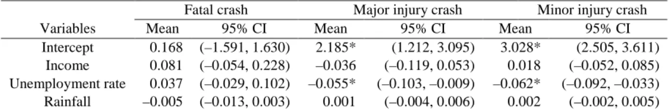
Table 6 Estimated parameters of the SMBYMTMRW1 model with all covariates
Variables
Fatal crash Major injury crash Minor injury crash
Mean 95% CI Mean 95% CI Mean 95% CI
Intercept 0.168 (–1.591, 1.630) 2.185* (1.212, 3.095) 3.028* (2.505, 3.611)
Income 0.081 (–0.054, 0.228) –0.036 (–0.119, 0.053) 0.018 (–0.052, 0.085)
Unemployment rate 0.037 (–0.029, 0.102) –0.055* (–0.103, –0.009) –0.062* (–0.092, –0.033) Rainfall –0.005 (–0.013, 0.003) 0.001 (–0.004, 0.006) 0.002 (–0.002, 0.005)
Snowfall –0.002 (–0.006, 0.003) –0.001 (–0.004, 0.002) 0.000 (–0.002, 0.001) TH32 0.001 (–0.005, 0.008) 0.000 (–0.004, 0.004) 0.000 (–0.002, 0.002) VMT 0.732* (0.538, 0.903) 0.970* (0.746, 1.160) 1.132* (0.893, 1.301) 𝜎𝜎2 𝜐𝜐 0.305 (0.103, 0.644) 0.412 (0.116, 0.903) 0.491 (0.136, 1.088) 𝜎𝜎2 𝜈𝜈 0.124 (0.067, 0.203) 0.188 (0.100, 0.299) 0.231 (0.124, 0.362) 𝑓𝑓𝑓𝑓𝐺𝐺𝑓𝑓𝜐𝜐 0.681 (0.383, 0.890) 0.651 (0.314, 0.889) 0.643 (0.305, 0.887) 𝜎𝜎2 𝜑𝜑 0.261 (0.081, 0.759) 0.253 (0.078, 0.708) 0.246 (0.078, 0.698) 𝜎𝜎2 𝜃𝜃 0.229 (0.074, 0.634) 0.214 (0.071, 0.576) 0.218 (0.072, 0.589) 𝑓𝑓𝑓𝑓𝐺𝐺𝑓𝑓𝜑𝜑 0.527 (0.219, 0.816) 0.533 (0.228, 0.820) 0.525 (0.226, 0.809) 𝑓𝑓𝑓𝑓𝐺𝐺𝑓𝑓 𝑆𝑆 𝑆𝑆+𝑇𝑇 0.487 (0.235, 0.718) 0.573 (0.314, 0.792) 0.618 (0.368, 0.813) 𝜎𝜎2 𝜂𝜂 0.047 (0.031, 0.067) 0.029 (0.022, 0.037) 0.018 (0.014, 0.022)
Note: CI, credible interval; TH32, number of days with minimum temperature exceeding 32°F; VMT, vehicle miles traveled; 𝜎𝜎2𝜐𝜐, 𝜎𝜎2𝜈𝜈, 𝜎𝜎2𝜑𝜑, 𝜎𝜎2𝜃𝜃, and 𝜎𝜎2𝜂𝜂 are variances; 𝑓𝑓𝑓𝑓𝐺𝐺𝑓𝑓𝜐𝜐 is the spatial fraction; 𝑓𝑓𝑓𝑓𝐺𝐺𝑓𝑓𝜑𝜑 is the temporal fraction; 𝑓𝑓𝑓𝑓𝐺𝐺𝑓𝑓 𝑆𝑆
𝑆𝑆+𝑇𝑇
is the relative importance of spatial effects; *covariates significant at the 95% credible interval.
4.1 Regression Coefficients Analysis
The intercept term was insignificant for fatal crashes but was significant for major injury and minor injury crashes. As expected, VMT showed significant positive effects for all three crash types. In addition, both intercept and VMT coefficients increased as crash injury severity decreased, which was consistent with the magnitude of crash counts.
Income was statistically insignificant for all three crash types, although income had generally increased for counties in Iowa from 2006 to 2015. Unemployment rate did not have significant effects on fatal crash counts but did have significantly negative effects on major injury and minor injury crash counts; that is, the number of major and minor injury crashes decreased as the unemployment rate increased. The unemployment rate has been thought to have mixed effects on traffic crash frequencies (Wagenaar, 1983; Leigh and Waldon, 1991). On one hand, high unemployment is associated with more mental stress in the population, related to both job loss and fear of job loss, which could lead to more aggressive driving patterns and more traffic crashes (Wagenaar, 1983). On the other hand, high unemployment also brings with it less driving and thus fewer traffic crashes (Wagenaar, 1983; Leigh and Waldon, 1991). The latter seemed to predominate in Iowa, which was consistent with what was found in Michigan, where unemployment had negative effects on crash counts (Wagenaar, 1983).
Rainfall, snowfall, and TH32 did not show significant effects on any crash type. Although these weather indicators had great variability within the time span studied, they were not related to traffic safety problems in the long term. Adverse weather, such as snowstorms and flooding, may result in more crashes in the short term but may also reduce people’s travel in the following time, leading to lower crash numbers. The two opposite effects seemed to offset each other.
It should be noted that all regression coefficients were assumed to be fixed for this study as shown in equation (3). That is, the effects of covariates on crash frequencies were thought to be homogeneous over space and time. However, these effects might be heterogeneous in practice in the presence of spatial instability and temporal instability, where fixed parameters models might
produce biased coefficient estimates and incorrect inferences (Mannering et al., 2016; Mannering, 2018). For example, snowfall might affect crash frequencies differently in rural areas and urban
areas due to different travel demands and travel modes. Thus, spatio-temporal-varying parameter
models might be considered to get more accurate results in future studies.
Because most covariates were found to be insignificant, the SMBYMTMRW1 model was re-run with
significant variables, and the results were shown in Table 7. The posterior p-values of the mean values of fatal, major injury, and minor injury crash counts for the new model were 0.493, 0.495, and 0.500, respectively, which meant it fitted the data well. Mean and 95% CI values of estimated parameters were found to be generally consistent with those shown in Table 6.
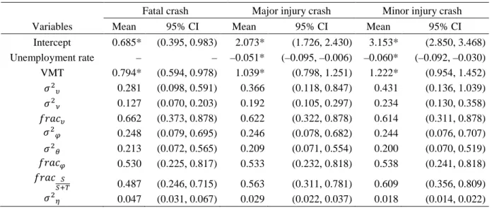
Table 7 Estimated parameters of the SMBYMTMRW1 model with significant covariates
Variables
Fatal crash Major injury crash Minor injury crash
Mean 95% CI Mean 95% CI Mean 95% CI
Intercept 0.685* (0.395, 0.983) 2.073* (1.726, 2.430) 3.153* (2.850, 3.468) Unemployment rate – – –0.051* (–0.095, –0.006) –0.060* (–0.092, –0.030) VMT 0.794* (0.594, 0.978) 1.039* (0.798, 1.251) 1.222* (0.954, 1.452) 𝜎𝜎2 𝜐𝜐 0.281 (0.098, 0.591) 0.366 (0.118, 0.847) 0.431 (0.136, 1.039) 𝜎𝜎2 𝜈𝜈 0.127 (0.070, 0.203) 0.192 (0.105, 0.297) 0.234 (0.130, 0.358) 𝑓𝑓𝑓𝑓𝐺𝐺𝑓𝑓𝜐𝜐 0.662 (0.373, 0.878) 0.622 (0.322, 0.878) 0.614 (0.311, 0.878) 𝜎𝜎2 𝜑𝜑 0.248 (0.079, 0.695) 0.246 (0.078, 0.682) 0.244 (0.076, 0.707) 𝜎𝜎2 𝜃𝜃 0.213 (0.072, 0.565) 0.209 (0.071, 0.554) 0.200 (0.070, 0.519) 𝑓𝑓𝑓𝑓𝐺𝐺𝑓𝑓𝜑𝜑 0.530 (0.225, 0.817) 0.533 (0.232, 0.818) 0.538 (0.241, 0.818) 𝑓𝑓𝑓𝑓𝐺𝐺𝑓𝑓 𝑆𝑆 𝑆𝑆+𝑇𝑇 0.487 (0.246, 0.715) 0.563 (0.311, 0.781) 0.609 (0.356, 0.809) 𝜎𝜎2 𝜂𝜂 0.047 (0.031, 0.067) 0.029 (0.022, 0.037) 0.018 (0.014, 0.022)
Note: CI, credible interval; VMT, vehicle miles traveled; 𝜎𝜎2𝜐𝜐, 𝜎𝜎2𝜈𝜈, 𝜎𝜎2𝜑𝜑, 𝜎𝜎2𝜃𝜃, and 𝜎𝜎2𝜂𝜂 are variances; 𝑓𝑓𝑓𝑓𝐺𝐺𝑓𝑓𝜐𝜐 is the spatial fraction; 𝑓𝑓𝑓𝑓𝐺𝐺𝑓𝑓𝜑𝜑 is the temporal fraction; 𝑓𝑓𝑓𝑓𝐺𝐺𝑓𝑓 𝑆𝑆
𝑆𝑆+𝑇𝑇
is the relative importance of spatial effects; *covariates significant at the 95% credible interval.
4.2 Random Effects Analysis
4.2.1 Spatial Random Effects Analysis
For the SMBYMTMRW1 model, the spatial fraction values for fatal, major injury, and minor injury
crashes were 0.662, 0.622, and 0.614, respectively. This means that, for all three crash types, unobserved heterogeneity in space existed both between counties and within individual counties, and the structured spatial effects played slightly more important roles than did the unstructured spatial effects. Shown in Figure 3 are the exponentials of the posterior means of the structured spatial effects (exp(υ𝑠𝑠𝑠𝑠)) for each county for all three crash types; counties with exp(υ𝑠𝑠𝑠𝑠) lower than 1 tended to have fewer crashes and counties with exp(υ𝑠𝑠𝑠𝑠) greater than 1 tended to have more crashes. It is found that the counties located in the north and southwest regions of Iowa tended to have fewer fatal, major injury, and minor injury crashes. For fatal crashes, this finding is generally consistent with the empirically observed fatal crash distribution shown in Figure 1(a). However, for major injury and minor injury crashes, it is not obvious to see these trends in Figure 1(a) and
Figure 1(b). This finding is a good example showing that one main benefit of spatial analysis is the identification of the underlying spatial clustering of crashes.
Figure 3 Exponential posterior means of the structured spatial effect (𝐼𝐼𝑒𝑒𝑝𝑝(υ𝑠𝑠𝑠𝑠)) of crashes in Iowa
Moran’s I statistics of residuals of the SMBYMTMRW1 model were calculated to see if they still had
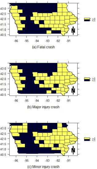
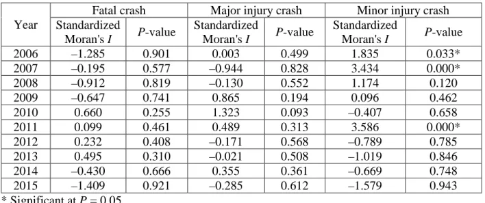
spatial correlations. As shown in Table 8, the residuals of fatal and major injury crashes did not show any significant spatial correlation at a 5% significance level for any year. In addition, the p -values were considerably larger than those shown in Table 3, which meant that unobserved heterogeneity in space was nearly completely covered by the spatial component. The p-values of Moran’s I test for the residuals of minor injury crashes also increased considerably in most years, which meant that the weak spatial autocorrelations of minor injury crashes were also eliminated. However, there were some exceptions in 2006, 2007, and 2011 for minor injury crashes, when the raw crash data did not show significant spatial autocorrelations, whereas their residuals showed significant spatial autocorrelations. It is thought that minor injury crashes might have trivial spatial autocorrelation in these three years but did have non-trivial spatial correlations in other years.
However, because the SMBYMTMRW1 model assigned fixed spatial random effects to the data for
each year, the residuals would also have spatial effects as the complement in these three years. This needs further investigation to determine the true reason. This finding implies the importance of checking the necessity of adopting spatial models in crash analysis. We suggest making spatial tests before and after spatial analysis to justify the utilization of spatial models. In general, the spatial component covered nearly all unobserved heterogeneity of crashes in space. The results also generally verified the effectiveness of the spatial model.
Table 8 Moran's I test results for the residuals of the 𝑆𝑆𝐵𝐵𝐵𝐵𝐵𝐵𝐵𝐵𝑇𝑇𝐵𝐵𝑅𝑅𝑅𝑅1 model Year
Fatal crash Major injury crash Minor injury crash Standardized Moran's I P-value Standardized Moran's I P-value Standardized Moran's I P-value 2006 –1.285 0.901 0.003 0.499 1.835 0.033* 2007 –0.195 0.577 –0.944 0.828 3.434 0.000* 2008 –0.912 0.819 –0.130 0.552 1.174 0.120 2009 –0.647 0.741 0.865 0.194 0.096 0.462 2010 0.660 0.255 1.323 0.093 –0.407 0.658 2011 0.099 0.461 0.489 0.313 3.586 0.000* 2012 0.232 0.408 –0.171 0.568 –0.789 0.785 2013 0.495 0.310 –0.021 0.508 –1.019 0.846 2014 –0.430 0.666 0.355 0.361 –0.669 0.748 2015 –1.409 0.921 –0.285 0.612 –1.579 0.943 * Significant at P = 0.05.
4.2.2 Temporal Random Effects Analysis
For the SMBYMTMRW1 model, the temporal fraction values for fatal, major injury, and minor injury
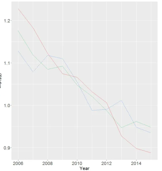
crashes were 0.530, 0.533, and 0.538, respectively. The structured temporal effects and the unstructured temporal effects played nearly the same roles for all three crash types. Thus, unobserved heterogeneity in time existed both between years and in individual years. Shown in Figure 4 are the exponentials of the posterior means of the structured temporal effects (exp(φ𝑠𝑠𝑠𝑠)) in each year for all three crash types. All three crash types generally showed descending trends from 2006 to 2015, whereas major injury and minor injury crashes had some fluctuations.
Figure 4 Exponential posterior means of the structured temporal effects (𝐼𝐼𝑒𝑒𝑝𝑝(φ𝑠𝑠𝑠𝑠)) of the SMBYMTMRW1 model
4.2.3 Spatial and Temporal Random Effects Comparison The 𝑓𝑓𝑓𝑓𝐺𝐺𝑓𝑓 𝑆𝑆
𝑆𝑆+𝑇𝑇
values for fatal, major injury, and minor injury crashes were 0.487, 0.563, and 0.609, respectively. This means that temporal effects played slightly more important roles for fatal crashes, whereas spatial effects played slightly more important roles for major injury and minor injury crashes. That is, the relative importance of spatial effects and temporal effects varied slightly by crash injury severity.
4.2.4 Unobserved Heterogeneity across Crash Injury Severities
The estimated variance–covariance matrices for all the random effects and the corresponding 95% credible intervals of the SMBYMTMRW1 model are shown in Table 9.
Table 9 Estimated variance-covariance matrices of the SMBYMTMRW1 model
Structured spatial effects (υ𝑠𝑠.)
Σ𝜐𝜐 Fatal crash Major injury crash Minor injury crash
Fatal crash 0.281 (0.098, 0.591)
Major injury crash 0.235 (0.035, 0.594) 0.366 (0.118, 0.847)
Minor injury crash 0.253 (0.035, 0.661) 0.322 (0.063, 0.850) 0.431 (0.136, 1.039) Unstructured spatial effects (𝜈𝜈𝑠𝑠.)
Σ𝜈𝜈 Fatal crash Major injury crash Minor injury crash
Fatal crash 0.127 (0.070, 0.203)
Major injury crash 0.110 (0.046, 0.190) 0.192 (0.105, 0.297)
Minor injury crash 0.121 (0.051, 0.207) 0.173 (0.082, 0.279) 0.234 (0.130, 0.358) Structured temporal effects (𝜑𝜑𝑠𝑠.)
Σ𝜑𝜑 Fatal crash Major injury crash Minor injury crash Fatal crash 0.248 (0.079, 0.695)
Major injury crash 0.001 (–0.223, 0.231) 0.246 (0.078, 0.682)
Minor injury crash –0.003 (–0.235, 0.227) –0.009 (–0.257, 0.208) 0.244 (0.076, 0.707) Unstructured temporal effects (𝜃𝜃𝑠𝑠.)
Σ𝜃𝜃 Fatal crash Major injury crash Minor injury crash
Fatal crash 0.213 (0.072, 0.565)
Major injury crash –0.002 (–0.193, 0.191) 0.209 (0.071, 0.554)
Minor injury crash –0.003 (0.182, 0.173) –0.007 (–0.186, 0.159) 0.200 (0.070, 0.519) Spatio-temporal interaction effects (𝜂𝜂(𝑠𝑠𝑠𝑠).)
Σ𝜂𝜂 Fatal crash Major injury crash Minor injury crash Fatal crash 0.047 (0.031, 0.067)
Major injury crash 0.002 (–0.007, 0.010) 0.029 (0.022, 0.037)
Minor injury crash 0.000 (–0.005, 0.006) 0.006 (0.002, 0.010) 0.018 (0.014, 0.022) Note: Values shown are the posterior mean with the 95% credible interval in parentheses; Σ𝜐𝜐, Σ𝜈𝜈,
Σ𝜑𝜑, Σ𝜃𝜃, Σ𝜂𝜂 are variance–covariance matrices of structured spatial effects, unstructured spatial
effects, structured temporal effects, unstructured temporal effects, and spatio-temporal interaction effects, respectively.
For the SMBYMTMRW1 model, unobserved heterogeneity across crash injury severities had three
sources: space, time, and spatio-temporal interaction. All the off-diagonal elements of Σ𝜐𝜐 and Σ𝜈𝜈 were significantly positive, which meant there were strong positive correlations across crash injury severities for both structured and unstructured spatial effects. That is, with the increase of fatal crash counts in one county, the major injury and minor injury crash counts of this county, and the fatal, major injury, and minor injury crash counts of its neighboring counties were also expected to increase. This proves the necessity of using multivariate spatial models from another viewpoint. However, none of the off-diagonal elements of Σ𝜑𝜑 and Σ𝜃𝜃 were significantly different from zero, which implied that there were no strong correlations across crash injury severities for either structured or unstructured temporal effects. However, the DIC value of the SMBYMTMRW1 model
was still much smaller than that for the SMBYMTRW1 model (shown in Table 5). This implies that,
although crashes may not show strong correlations in time, their correlations may still not be ignored, as weak correlations may still explain some variability in the data. For the spatio-temporal interaction effects, major injury crashes showed significantly positive correlations with minor injury crashes, but fatal crashes did not show significant correlations with the other two crash types. For each observation, because Σ𝜐𝜐, Σ𝜈𝜈, Σ𝜑𝜑, Σ𝜃𝜃, 𝐺𝐺𝑃𝑃𝑖𝑖Σ𝜂𝜂 are independent, the Pearson’s correlation coefficients of random effects across crash injury severities can be calculated as follows:
𝜌𝜌12= Σ𝜐𝜐12+Σ𝜈𝜈12+Σ𝜑𝜑12+Σ𝜃𝜃12+Σ𝜂𝜂12 �σ2𝜐𝜐1+σ2𝜈𝜈1+σ2𝜑𝜑1+σ2𝜃𝜃1+σ2𝜂𝜂1�σ2𝜐𝜐2+σ2𝜈𝜈2+σ2𝜑𝜑2+σ2𝜃𝜃2+σ2𝜂𝜂2 (23) 𝜌𝜌13= Σ𝜐𝜐13+Σ𝜈𝜈13+Σ𝜑𝜑13+Σ𝜃𝜃13+Σ𝜂𝜂13 �σ2𝜐𝜐1+σ2𝜈𝜈1+σ2𝜑𝜑1+σ2𝜃𝜃1+σ2𝜂𝜂1�σ2𝜐𝜐3+σ2𝜈𝜈3+σ2𝜑𝜑3+σ2𝜃𝜃3+σ2𝜂𝜂3 (24) 𝜌𝜌23 = Σ𝜐𝜐23+Σ𝜈𝜈23+Σ𝜑𝜑23+Σ𝜃𝜃23+Σ𝜂𝜂23 �σ2𝜐𝜐2+σ2𝜈𝜈2+σ2𝜑𝜑2+σ2𝜃𝜃2+σ2𝜂𝜂2�σ2𝜐𝜐3+σ2𝜈𝜈3+σ2𝜑𝜑3+σ2𝜃𝜃3+σ2𝜂𝜂3 (25)
where 𝜌𝜌12 is the Pearson correlation coefficient of random effects between fatal and major injury crashes, 𝜌𝜌13 is the Pearson correlation coefficient of random effects between fatal and minor injury crashes, and 𝜌𝜌23 is the Pearson correlation coefficient of random effects between major injury and minor injury crashes.
The posterior means and 90% credible intervals of Pearson correlation coefficients of random effects are shown in Table 10. The Pearson correlation coefficient between any two crash types was significantly positive at a 90% credible interval, but the Pearson correlation coefficient between major injury and minor injury crashes was generally larger than the other two values. That is, major injury and minor injury crashes had a stronger correlation compared to fatal crashes, which was consistent with the Pearson correlation coefficients of crash counts shown in Table 2.
Table 10 Pearson correlation coefficients of random effects across crash injury severities Pearson correlation coefficient Mean 90% CI
𝜌𝜌12 0.357 (0.047, 0.605)
𝜌𝜌13 0.366 (0.066, 0.605)
𝜌𝜌23 0.453 (0.145, 0.689)
Note: CI, credible interval; 𝜌𝜌12, 𝜌𝜌13, 𝜌𝜌23, Pearson correlation coefficients between fatal and major injury crashes, between fatal and minor injury crashes, and between major injury and minor injury crashes, respectively.
4.3 Site Ranking Results Analysis
The crude crash rates and the predicted crash rates for all three crash types, which were calculated by dividing the crash counts by VMT, are shown in Figure 5. A linear regression model was built to check their correlation.
Figure 5 Crude crash rate versus predicted crash rate of fatal, major injury, and minor injury crashes
The 𝑅𝑅2 value was 0.929, which means that the crude crash rates were generally consistent with the predicted crash rates. Specifically, for major injury and minor injury crashes, these two rates were very consistent, but for fatal crashes, they were inconsistent. Major injury and minor injury crash counts were very large, but fatal crash counts were very small, as shown in Table 1. Thus, occurrences of fatal crashes were more stochastic than major injury and minor injury crashes. It is thought that the multivariate structure could borrow information from major injury and minor injury crashes to estimate fatal crashes stably (Boulieri et al., 2017). Thus, the predicted data from the SMBYMTMRW1 model are expected to be smoother for unstable low-frequency fatal crashes, and
could represent the underlying true distribution of fatal crashes better than the crude data could. The crash cost rates directly influenced the ranking results shown in Figure 6, where x-axis showed the crude rank by the crude crash cost rate and y-axis showed the PER by the predicted crash cost rate. The two ranking methods produced consistent results for major injury and minor injury crashes but had large differences for fatal crashes, which led to different ranking results for total crashes.
Figure 6 County rank by crude crash cost rate versus county posterior expected rank by predicted crash cost rate in 2015
The top 10 risky counties using the two ranking methods are shown in Figure 7. Of the counties ranked by these two methods, seven appeared in the top 10 for both methods, whereas three counties appeared only in the top 10 of one or the other method; Lyon, Hamilton, and Mahaska Counties were in the top 10 list using the predicted crash cost rate PER but not in the crude crash cost rate ranking. Moreover, the rank orders of the seven counties appearing in both top 10 lists were also very different. For example, the highest ranked county by the crude crash cost rate, Marion County, was ranked only eighth by the PER of the predicted crash cost rate. The big differences between the two ranking methods show the importance of the multivariate spatio-temporal Bayesian model, which is expected to better identify the underlying true status quo of traffic safety. The top 10 risky counties shown in Figure 7(b) should be the focus of future safety improvement programs.
5
Discussion and Conclusions
Unobserved heterogeneity of crashes over space and time is often a big issue in crash frequency analysis. When multiple crashes are analyzed, correlations across crash types may also produce unobserved heterogeneity, which may exist in space, time, and space–time interactions. In this study, we used the multivariate spatio-temporal Bayesian model to analyze the yearly county-level fatal, major injury, and minor injury crash counts in Iowa from 2006 to 2015. Income, rainfall, snowfall, and temperature did not have significant influences on the frequencies of any of the three crash types, whereas unemployment rate showed significantly negative influences on major injury and minor injury crash counts, and VMT showed significantly positive influences on all three crash types.
All three crash types showed very strong spatial correlations. The counties located in northern and southwestern Iowa tended to have fewer crashes, whereas the remaining counties tended to have more crashes. All three crash types generally showed descending trends from 2006 to 2015. Both spatial and temporal effects were non-negligible, and they played nearly the same roles for all three crash types with slight differences. In addition, all three crash types showed significantly positive correlations between each other across space but not across time. The crude data and the predicted data were generally consistent for major injury and minor injury crashes but were very different for fatal crashes, the crude data of which were more stochastic due to the low counts. The predicted data from the multivariate spatio-temporal model were smoother than were the crude data. The crash cost rates were calculated based on crash rates and crash costs by injury severity and were used as ranking indicators. Two ranking methods, crude rank by the crude crash cost rate and PER by the predicted crash cost rate, were presented to identify the counties with higher risks for traffic safety. The two methods produced very different ranking results, and the latter method was thought to be able to better represent the true status quo of traffic safety. The ranking results would be helpful for transportation agencies drawing up traffic safety improvement programs in the future. In future research, the data may be analyzed using smaller space and time scales, which would produce more targeted and practical findings. In addition, as shown in Table 3, the spatial correlations of all three crashes were different in different years. That is, the spatial correlations may evolve dynamically over time. Similar situations may also appear in temporal correlations, whereby the descending rates of crashes in different counties may be different. Thus, dynamic spatio-temporal models should be considered in future studies. Meanwhile, in this study, only random effects were thought to be correlated in space and time, but regression coefficients might also be correlated in space and time. Thus, future researchers may want to consider spatio-temporal-varying coefficient models. It is suggested that the review by Mannering (2018) about temporal instability in accident analysis be consulted for more ideas. All the above-mentioned directions would need more data or more complex statistical models, so computation may be a big concern, especially when using MCMC simulation to estimate Bayesian models. Some emerging fast Bayesian estimation tools, such as integrated nested Laplace approximation (Rue et al., 2009), should be considered. As was shown in this study, care should also be taken in the selection of appropriate priors and initial values for MCMC simulations. Finally, for this study we adopted two common spatial and temporal models; however, there are many other spatial and temporal models
available. Future researchers may also explore the effectiveness of other models in crash frequency analysis.
6
References
Aguero-Valverde, J., 2011. Direct spatial correlation in crash frequency models. 3rd International Conference on Road Safety and Simulation, Indianapolis, IN, USA.
Aguero-Valverde, J., 2013. Multivariate spatial models of excess crash frequency at area level: Case of Costa Rica. Accident Analysis and Prevention 59, 365–373.
Aguero-Valverde, J., Jovanis, P.P., 2006. Spatial analysis of fatal and injury crashes in Pennsylvania. Accident Analysis and Prevention 38 (3), 618–625.
Aguero-Valverde, J., Jovanis, P.P., 2008. Analysis of road crash frequency with spatial models. Transportation Research Record 2061, 55–63.
Aguero-Valverde, J., Jovanis, P.P., 2010. Bayesian multivariate Poisson lognormal models for crash severity modeling and site ranking. Transportation Research Record 2136, 82–91. Aguero-Valverde, J., Wu, K.F., Donnell, E.T., 2016. A multivariate spatial crash frequency model
for identifying sites with promise based on crash types. Accident Analysis and Prevention 87, 8–16.
Ahmed, M.M., Abdel-Aty, M., 2015. Evaluation and spatial analysis of automated red-light running enforcement cameras. Transportation Research Part C 50, 130–140.
Andrey, J., 2010. Long-term trends in weather-related crash risks. Journal of Transport Geography 18 (2), 247–258.
Anselin, L., 1988. Spatial Econometrics: Methods And Models. Springer, Netherlands.
Barua, S., El-Basyouny, K., Islam, M.T., 2016. Multivariate random parameters collision count data models with spatial heterogeneity. Analytic Methods in Accident Research 9, 1–15. Besag, J., York, J., Mollié, A., 1991. Bayesian image restoration, with two applications in spatial
statistics. Annals of the Institute of Statistical Mathematics 43 (1), 1–20.
Bivand, R., Piras, G., 2015. Comparing implementations of estimation methods for spatial econometrics. Journal of Statistical Software 63 (18), 1–36.
Blangiardo, M., Cameletti, M., Baio, G., Rue, H., 2013. Spatial and spatio-temporal models with R-INLA. Spatial and Spatio-temporal Epidemiology 4, 33–49.
Boulieri, A., Liverani, S., Hoogh, K. de, Blangiardo, M., 2017. A space–time multivariate
Bayesian model to analyse road traffic accidents by severity. Journal of the Royal Statistical
Society Series A 180 (1), 119–139.
Brijs, T., Karlis, D., Wets, G., 2008. Studying the effect of weather conditions on daily crash counts using a discrete time-series model. Accident Analysis and Prevention 40 (3), 1180–1190.
Eckley, D.C., Curtin, K.M., 2013. Evaluating the spatiotemporal clustering of traffic incidents. Computers, Environment and Urban Systems 37, 70–81.
El-Basyouny, K., Barua, S., Islam, M.T., 2014. Investigation of time and weather effects on crash types using full Bayesian multivariate Poisson lognormal models. Accident Analysis and Prevention 73, 91–99.
El-Basyouny, K., Sayed, T., 2009. Collision prediction models using multivariate Poisson-lognormal regression. Accident Analysis and Prevention 41 (4), 820–828.
Erdogan, S., 2009. Explorative spatial analysis of traffic accident statistics and road mortality among the provinces of Turkey. Journal of Safety Research 40 (5), 341–351.
Gelman, A., Meng, X.-L., Stern, H., 1996. Posterior predictive assessment of model fitness via realized discrepancies. Statistica Sinica 6 (4), 733–807.
Gelman, A., Rubin, D.B., 1992. Inference from iterative simulation using multiple sequences. Statistical Science 7 (4), 457–511.
Guo, F., Wang, X., Abdel-Aty, M.A., 2010. Modeling signalized intersection safety with corridor-level spatial correlations. Accident Analysis and Prevention 42 (1), 84–92.
Hu, S., Ivan, J.N., Ravishanker, N., Mooradian, J., 2013. Temporal modeling of highway crash counts for senior and non-senior drivers. Accident Analysis and Prevention 50, 1003–1013. Iowa Community Indicators Program, 2016. Iowa Community Indicators Program (ICIP).
http://www.icip.iastate.edu/ (accessed 2.20.17).
Iowa Department of Transportation, 2016. Vehicle-miles traveled (VMT). http://www.iowadot.gov/maps/msp/vmt/vmt.html (accessed 10.20.16).
Iowa Environmental Mesonet, 2017. Iowa Environmental Mesonet (IEM). https://mesonet.agron.iastate.edu/ (accessed 2.20.17).
Jiang, X., Abdel-Aty, M., Alamili, S., 2014. Application of Poisson random effect models for highway network screening. Accident Analysis and Prevention 63, 74–82.
Kilamanua, W., Xia, J., Caulfieldb, C., 2011. Analysis of spatial and temporal distribution of single and multiple vehicle crash in Western Australia: a comparison study. 19th International Congress on Modelling and Simulation, Perth, Australia.
Leigh, J.P., Waldon, H.M., 1991. Unemployment and highway fatalities. Journal of Health Politics, Policy and Law 16 (1), 135–156.
Liu, C., Gyawali, S., Sharma, A., Smaglik, E., 2015. A methodological approach for spatial and temporal analysis of red light running citations and crashes: a case-study in Lincoln, Nebraska. Transportation Research Board 94th Annual Meeting, Washington, D.C., USA.
Liu, C., Sharma, A., 2017. Exploring spatio-temporal effects in traffic crash trend analysis. Analytic Methods in Accident Research 16, 104–116.
Lord, D., Mannering, F., 2010. The statistical analysis of crash-frequency data: a review and assessment of methodological alternatives. Transportation Research Part A 44 (5), 291–305.