Inverse Correspondence Analysis
Patrick J.F. Groenen
∗Michel van de Velden
†September 10, 2002
Econometric Institute Report EI 2002-31
∗Econometric Institute, Erasmus University Rotterdam, The Netherlands, P.O. Box
1738, 3000 DR Rotterdam, The Netherlands (e-mail: [email protected]).
Abstract
In correspondence analysis, rows and columns of a data matrix are depicted as points in low-dimensional space. The row and column profiles are approximated by minimizing the so-called weighted chi-squared distance between the original profiles and their approxima-tions, see or example, Greenacre (1984). In this paper, we will study the inverse correspondence analysis problem, that is, the possibili-ties of retrieving one or more data matrices from a low dimensional correspondence analysis solution. We will show that there exists a nonempty closed and bounded polyhedron of such matrices. We also present an algorithm to find the vertices of the polyhedron. A proof that the maximum of the Pearson chi-squared statistic is attained at one of the vertices is given. In addition, it is discussed how extra equality constraints on some elements of the data matrix can be im-posed on the inverse correspondence analysis problem. As a special case, we present a method for imposing integer restrictions on the data matrix as well. The approach to inverse correspondence analysis fol-lowed here is similar to the one employed by De Leeuw and Groenen (1997) in their inverse multidimensional scaling problem.
Keywords: Correspondence Analysis, Inverse Problems, Maximum Chi-Square.
1
Introduction
In correspondence analysis (CA), the rows and columns of a data matrixFare depicted as points in low-dimensional space. Most often, Fis a contingency matrix, but this need not be the case. The only restriction on F is that its elements are nonnegative. A CA solution is obtained by simultaneously approximating the row and column profiles through minimization of the so-called chi-squared distance. It is well known that the CA solution for both the rows and columns can be obtained immediately from the singular value decomposition of the scaled data matrix.
Much is known about the properties of CA, see, for example, Greenacre (1984), Gifi (1990), and Van de Velden (2000). In this paper, we concentrate on a problem that has not been treated before. Given a low dimensional CA solution, which matricesFwould have produced the current solution as a CA solution? We call this problem the inverse correspondence analysis problem. There are several reasons to investigate the inverse CA problem. First of all, the size of the set of matrices F may reveal information about the uniqueness of the original solution. If this set is large, then there are many nonnegative matrices Fthat yield the same CA solution. Thus, even though the data have lead to a perfectly normal correspondence analysis solution, it is good to realize that there are many other data sets that would have led to exactly the same solution. On the other hand, if the set is small, there are much less nonnegative matrices F yielding the solution of the original prob-lem. In particular, if the set only consists of the original data, then we know that there is a unique relation between the correspondence analysis solution and the data. Second, when CA solutions are reported in the literature, the original data are not always presented. The solution of the inverse CA problem enables us to generate data that has the original CA solution as its CA solution. These generated data can then be used in simulation studies. Thirdly, we believe that the study of inverse CA deepens our understanding of CA. Finally, through inverse CA, we are able to prove the upper bound of the Pearson chi-square given marginal frequencies but unknown data.
To study the inverse CA problem, we will follow a similar approach to the one proposed by De Leeuw and Groenen (1997), in their treatment of the inverse multidimensional scaling problem (see also, Groenen, De Leeuw, & Mathar, 1996).
This paper is organized as follows. First, we introduce notation for CA. Then we formalize the inverse CA problem. Next, we present a computational method for computing the inverse CA solution. Then, we discuss where the upper bound of the Pearson chi-square statistic is attained. The next section discusses how additional equality and integer constraints can be imposed.
We illustrate our method by an example. This paper is ended with some concluding remarks.
2
The Correspondence Analysis Problem
Before we start with the inverse CA problem, let us introduce notation needed for CA. Let F denote an nr ×nc matrix of nonnegative elements on which
CA is performed. Let r be the vector of row sums ofF, that is, r =F1 and c the vector of columns sums, c=F01, where 1 denotes a vector of ones of
appropriate length. Furthermore, define n as the sum of all elements of F, that is, n=10F1.
Define the scaled data matrixF˜ asF˜ =D−1/2
r FD−c1/2, where Dr and Dc
are diagonal scaling matrices with, respectively, the elements of r and c on their diagonal. The task of correspondence analysis is to find k-dimensional coordinates matrices R and Cfor row and column points such that the loss function
φ(Rk,Ck) =kF˜−Dr1/2RkC0kD1c/2k2 (1)
is minimized, where kAk2 denotes the sum of squared elements of A. Con-sider the (complete) singular value decomposition
˜
F=UΛV0, where U0U=I
nr,V
0V =I
nc, (2)
whereIi denotes thei×iidentity matrix. Then, by Eckart and Young (1936)
we can minimize φ(Rk,Ck) by
Rk =D−r1/2UkΛαk and Ck =D−c1/2VkΛ1k−α,
where Uk and Vk are respectively the nr×k andnc×k matrices of singular
vectors corresponding to the k largest singular values gathered in the k×k
diagonal matrix Λk, and α is a nonnegative scalar. Clearly,
R0kDrRk =Λ2kα and C0kDcCk=Λ2(1k −α).
For α = 1, we obtain row principal coordinates and for α = 0 column prin-cipal coordinates.
Now, suppose that the marginalsrand cand the coordinatesRkand Ck
are given. Then, the inverse correspondence analysis problem is concerned with the question what matrix F could have produced Rk and Ck as its
CA solution. In other words, given a CA solution, can we find one or more matrices Fthat have the given CA solution as its CA solution?
In the next section, we shall investigate the properties of the setF satisfy-ing the requirements for inverse CA. Necessarily, F must contain the original data matrix F as an element. We assume, without loss of generality, that
nr ≥ nc, so that the rank of F equals nc or less. If k = nc, the inverse
CA problem is trivial and set F only contains F. For k < nc, however, the
problem is not trivial and is discussed below.
3
Formalizing the Inverse Correspondence
Anal-ysis Problem
Suppose that we have a correspondence analysis solution Rk and Ck in k
dimensions. In addition, we will assume throughout this paper that the row and column sums of F are known, so that the scaling matrices Dr and Dc
are known. Note that these vectors of row and column totals are of great importance in correspondence analysis. Not only do they provide the proper scaling for the coordinates, they are also referred to as the called trivial so-lution, see, e.g., Greenacre (1984). Typically, one ignores this trivial soso-lution, which can be done by simply discarding the solution, or by considering the singular value decomposition of D−1/2
r (F−n−1rc0)D−c1/2 rather than that
of D−1/2
r FD−c1/2. In the following, we will assume that the trivial solution
is contained in the coordinate matrices Rk and Ck. Hence, we will consider
the singular value decomposition of F˜ for 1≤k ≤nc.
In the inverse CA problem, we look for all Fthat have
1. column sum c and row sum r, that is, F1=cand 10F=r,
2. Rk and Ck in its CA solution, and
3. only nonnegative elements.
Note that condition 2 does not imply that CA on a particularFyieldsRkand
Ckas thefirstkdimensions. Condition 2 only tells us thatRk andCkwill be
among the CA dimensions. In the strict inverse CA problem, the additional condition imposed is that Rk and Ck must be the first k dimensions. In the
remainder of this section, we investigate properties of the (strict) inverse CA problem.
Recall the complete singular value decomposition ˜ F=UΛV0, where U0U=I nr,V 0V =I nc. (3) Let U= [Uk | Uc], V = [Vk | Vc] and Λ= " Λk 0 0 Λc # ,
whereUcisnr×(nr−k),Vc isnc×(nc−k) andΛcis an (nr−k)×(nc−k)
matrix that can be partitioned asΛc= [Λ˜c 0]0 whereΛ˜c is diagonal of order
(nc−k)×(nc−k) and, generically,0denotes a matrix of zeros of appropriate
order. Furthermore, as U0U=I
nr and V
0V=I
nc it follows that
U0kUc=0and V0kVc=0. (4)
Assuming for the moment that Fis known, then the complete singular value decomposition for the scaled matrix F˜ = D−1/2
r FD−c1/2 can be expressed in
the following way ˜
F=UΛV0 =UkΛkV0k+UcΛcVc0.
Now assume that F and thus F˜ are unknown, but Rk,Ck,Dr,Dc and thus
UkΛkV0k are known. From the orthogonality restrictions (4) we can obtain
matrices U˜c = UcT and V˜c =VcQ, where T and Q are unknown
orthog-onal matrices of the appropriate orders. Then, F˜ is decomposed into two orthogonal parts
˜
F=UkΛkVk0 +U˜cG ˜Vc0, (5)
where G= T0Λ
cQ. From (5) it can easily be derived that F can be
recon-structed as
F=D1r/2(UkΛkVk0 +U˜cG ˜Vc0)D1c/2. (6)
Therefore, in the inverse correspondence analysis problem, we search for those matrices Gfor which F reconstructed by (6) satisfies the three earlier mentioned conditions.
Lemma 1 For anyG, the matrix F˜ reconstructed by (5) has singular values
Λk and corresponding matrices of singular vectors Uk and Vk.
Proof. The matrices of singular vectors Uk and Vk, are matrices of
eigen-vectors ofF˜˜F0 andF˜0F˜ respectively. From (4) it follows immediately that for
any F˜ reconstructed using (5) we haveF˜˜F0U
k =UkΛ2k andF˜0FV˜ k =VkΛ2k.
Lemma 2 For anyG, the matrixFreconstructed by (6) has row sums equal to r and column sums equal to c.
Proof. This follows immediately from Lemma 1 and the fact that the trivial solution in correspondence analysis (that is, the first dimension) is equal to
λ1u1v01 =n−1Dr1/2110Dc1/2. Pre multiplying byD1r/2 and post multiplying by
D1/2
r gives n−1Dr110Dc = n−1rc0, so that the row sums equal n−1rc01 = r
Lemma 1 tells us that any G inserted in (6) gives a CA decomposition that includes the original Rk and Ck. However, without any additional
constraints on Gsome of the elements ofF may become negative. Thus, we have additional restrictions on G to make the elements of F nonnegative. Note that ifG is constrained so that all elements ofF˜ are nonnegative, then F must have nonnegative elements as well, since F=D−1/2
r FD˜ −c1/2 and Dr
and Dc have nonnegative elements only. To meet these extra constraints
all elements of U˜cG ˜V0c must be larger than (or equal to) the elements of
−UkΛkVk0.
Let g = vec(G), where the vec operator stacks the columns of G below each other. Using the relationship
vec(ABC) = (C0⊗A) vec(B) (7)
between the vec operator and the Kronecker product, we can express the nonnegativity restrictions as
Cg≥ −d (8)
where C=V˜c⊗U˜c and d = vec(UkΛkV0k).
Lemma 3 The system of inequalities (8) is consistent.
Proof. Choosing G = T0Λ
cQ reconstructs the original F. Therefore, the
set of matrices Gor vectors g satisfying (8) is nonempty. Thus, the system of inequalities (8) is consistent.
Theorem 4 The solution setF of the inverse correspondence analysis prob-lem is a convex set.
Proof. Each inequality in (8) defines a convex half space. The intersection of convex sets is convex, so that F is convex, too.
Theorem 5 The set F is a bounded closed polyhedron.
Proof. The fact that F is a closed polyhedron follows immediately since it is an intersection of half spaces defined by the system of inequalities (8). Boundedness can be established if it can be proved that F does not contain a ray. If F contains a ray, then there exists a G1 in F such that βG1 ∈ F for β > 0. Let Ft denote the trivial solution, that is, Ft =n−1D1r/2110D1c/2,
and let Fc =U˜cG ˜Vc0. From (4) it follows that F0tFc= 0(nc×nc) and FtF
0
c=
0(nr×nr). As Ft is strictly positive, that is, all its elements are greater than
zero, it follows immediately that each row and column of Fcmust contain at
least one negative element. MultiplyingFc =UcGV0cwith a sufficiently large
β will make F contain one or more negative values so that F falls outside the polyhedron. Therefore, F does not contain a ray and is consequently bounded.
Lemma 6 EachF at the hull of the polyhedron has at least(nr−k)(nc−k)
values equal to zero.
Proof. The system of inequalities (8) is derived from the nonnegativity restrictions on the elements of F. Since G is an (nr−k)×(nc−k) matrix,
there are (nr−k)(nc−k) independent elements in g. Thus, any F at the
hull of the polyhedron corresponds to a g for which at least (nr−k)(nc−k)
of the inequalities are equalities. Since an equality in (8) corresponds to a zero element in F, there are at least (nr−k)(nc−k) zero elements in F at
the hull of the polyhedron.
Theorem 7 The setFstrict defined by strict inverse CA is a bounded convex
set.
Proof. Set Fstrict is an intersection between F and the set G of matricesG with singular values smaller than or equal to λk. To prove that the latter set
is convex, we use a result of Magnus and Neudecker (1988, p. 205) stating that the largest eigenvalueλ2
maxofG0Gdefines a convex function. Therefore, the set G of matrices Gwith λ2
max≤λ2k is convex. This property also holds
for strict monotone functions of λ2
max such as the square root. Therefore, the setGofG’s withλmax≤λk is convex as well. The intersection of two convex
sets is also convex, so that the intersection of F and G is convex. SinceF is bounded, Fstrict must also be bounded.
4
Computing the Inverse Map
In De Leeuw and Groenen (1997), a similar problem was investigated, the so-called inverse multidimensional scaling problem. Here, we take a similar computational approach.
The basic idea is to check all possible vertices of the system of inequalities defined by Cg ≥ −d. Let m = (nr −k)(nc−k) be the length of vector g.
Then, check for all ³nrnc
m
´
combinations of rows whether the combination defines a valid vertex.
The Inverse Correspondence Analysis Algorithm:
1. Let the set of vertices V be empty. 2. Do for all³nrnc
m
´
combinations ψ:
• Letgψ be the solution of the system Cψg=dψ.
• Check if Cgψ ≥d. If so, then add gψ to the set of vertices V.
4. End do.
Note that if someCψ is not of full rank, thenψ cannot be a vertex, so it
is simply discarded.
5
A strict upper bound for the Pearson
chi-squared statistic
Let χ2 denote the Pearson chi-squared statistic for testing independence. That is, χ2(F) = P
i
P
j(fij − eij)2/eij with eij = ricj/n. Note that the
r and c are known in advance. Now we can make use of the results for inverse CA to obtain the upper bound of the chi-squared statistic under the independence model. However, we first consider the general case of the maximum chi-squared statistic in inverse CA.
Theorem 8 The maximum χ2 over the inverse CA set F is attained at one
of the vertices.
Proof. Clearly, χ2(F) is quadratic in F so it is a convex function. Because Fis determined by Gthrough (6) andGmust be in the convex setF,Flies in a convex set too. Rockafellar (1970, Theorem 32.3, p. 344) states that the maximum of a convex function over a convex set is obtained at an extremal point. An extremal point of a convex set is a point that cannot be expressed as a convex combination of other points in the convex set (Rockafellar, 1970, p. 162). The extremal points of a polyhedron are the vertices. Because F is a polyhedron, the maximum χ2 is obtained at a vertex.
This theorem can also be used to obtain the maximum χ2 under the independence model, where only the the marginal frequencies r and c are given and no other CA dimension is known. In the independence case, too, the value χ2 is bounded above and the maximum is attained at one of the vertices. This situation arises in the inverse CA problem when only the trivial dimension is given so that k = 1. To obtain the maximum value, the algorithm from Section 4 can be used, although computationally (much) faster methods may exist that make efficient use of the additional structure in the restrictions.
6
Additional Constraints in Inverse CA
We now consider the case where, in addition to the marginals, extra infor-mation concerning elements ofFis available. First we discuss the case where one or more elements ofFare known. Then we present an algorithm that can be used to reduce the original set F under the restriction that the elements of the original matrix need to be integers.
6.1
Equality Constraints
It may occur that one or more elements ofFare knowna priori. For example, if a certain event cannot occur, the corresponding value in F must be zero. Assume thatpvalues ofF, and hence, ofF˜,are known. Letφ denote the row indices of Cfor which the equality constraints are imposed, so that the rows of the p×m matrix Cφ match the constrained rows of C. Furthermore, let
˜fφ denote the p×1 vector of corresponding (known) values of F˜ and let dφ
denote the corresponding rows of d. The new constraints can be expressed as
Cφg=˜fφ−dφ. (9)
Theorem 9 The solution of constrained inverse CA is a bounded convex polyhedron that may be empty.
Proof. By Theorem 5, the solution of the inverse CA problem defines a bounded convex polyhedron. The equality constraints defined by (9) are linear and thus convex. The union of a bounded polyhedron and a linear subspace is again a bounded polyhedron. Because the subspace may fall outside the polyhedron, e.g., by imposing an invalid constraint such as con-straining fij to be larger than either of the corresponding marginals ri or ci,
the union of the two sets may be empty.
We distinguish three cases that may occur with respect to the constraints as expressed in (9):
(a) p < m: There are fewer constraints than free elements in g. We can implement the restrictions in our algorithm in the following way.
The Constrained Inverse Correspondence Analysis Algorithm:
2. Do for all³nrnc−p
m−p
´
combinationsψ∗, where each combination
con-tains φ, i.e. ψ∗ = Ã φ ψ ! : 3. Let Cψ∗ = Ã Cφ Cψ ! and dψ∗ = Ã ˜fφ−dφ −dψ ! be the m rows of C and d, defined by ψ∗ and the constrained values˜f
φ.
• Letgψ∗ be the solution of the system Cψ∗g=dψ∗.
• Check if Cgψ∗ ≥d. If so, then add gψ∗ to the set of vertices
V. 4. End do.
(b) p=m: The number of constraints is equal to the number of unknown elements. Therefore, if the corresponding matrix Cφ is nonsingular,
that is, if C−1
φ exists, we obtain a unique solution for g. Thus, if F
reconstructed using (6) is nonnegative, we have a valid unique solu-tion. Else, if an element of the reconstructed matrix Fis negative, the solution set F is empty.
If Cφ is singular, that is, if some constraints are linearly dependent
and hence redundant, we cannot uniquely determine g. We thus have a similar situation as in (a). We can obtain vertices satisfying the equality and nonnegativity constraints in the following way: Let p∗
denote the rank ofCφ. Then, consider for all
³
nrnc−p
m−p∗ ´
combinations of rows of Cthat contain Cφ, the following system of equations:
Cφ∗g=˜fφ∗−dφ∗
where Cφ∗ is a (2p−p∗)×m matrix with as first p rows independent
rows of C corresponding to the equality constraints, ˜fφ∗ is the vector
˜fφ supplemented with p−p∗ zeros anddφ∗ is the vector of appropriate
elements of d. Then, for each Cφ∗ that has rank m, we can calculate
g as g= (C0
φ∗Cφ∗)−1Cφ0∗(˜fφ∗−dφ∗). Upon checking the nonnegativity
constraintsCg≥d, we add or discard the vertices to our solution set. Note that, if Cφ∗ is not of full column rank then φ∗ cannot be a vertex
and we can simply discard it.
(c) p > m: There are more constraints than free elements, so that the matrix Cφ has more rows than columns. Then, assuming that Cφ has
full column rank,g can be calculated asg= (C0
φCφ)−1C0φ(˜fφ−dφ). In
order for g to be a valid solution, F reconstructed using (6) must be nonnegative. Else, the solution set F is empty.
If the rank of Cφ is smaller than m, we have essentially the same
situation as described under (b) and we can apply the same procedure to obtain vertices.
Note that, by imposing the additional constraints, we have decreased the number of inequalities to be checked. Therefore, with a sufficient number of constraints even large inverse CA problems become computationally feasible.
6.2
Integer constraints
Suppose we know that the elements of the original matrix F are integers. For example, we may know F to be a contingency matrix. This information can be used to reduce the solution set F in the following way.
Let Fh denote the reconstructed matrix for the h-th vertex g
h, that is
Fh = D−1/2
r (UkΛkV0k +U˜cGhV˜0c)D−c1/2, where vec(Gh) = gh and let fijh
denote the ij-th element of Fh. Define int
+(x) as the first integer larger than x and int−(x) as the first integer smaller than x. Also, let Fmin be the matrix with elements int+(minh(fijh)) (that is, the smallestij-th element
over all vertices) andFmaxhave elements int−(maxh(fijh)) (that is, the largest
ij-th element over all vertices).
Theorem 10 When F is restricted to have elements fij that are integer,
then elements of F are bounded below by Fmin and bounded above by Fmax. Proof. This follows directly from the convexity of the solution set F in Theorem 4 and the integer constraint for the elements of F.
DefineF˜min =D−r1/2FminD−c1/2,F˜max=Dr−1/2FmaxDc−1/2,˜fmax= vec(F˜max), and˜fmin = vec(F˜min). Using (6), we must have
˜
Fmin−UkΛkV0k ≤U˜cG ˜Vc0 ≤F˜max−UkΛkV0k,
or in vec notation
˜fmin−d≤Cg≤˜fmax−d.
These additional integer restrictions can be implemented as follows:
The Integer Constrained Inverse Correspondence Analysis Algorithm:
1. Find an initial set of verticesV by the Inverse Correspondence Analysis Algorithm of Section 4.
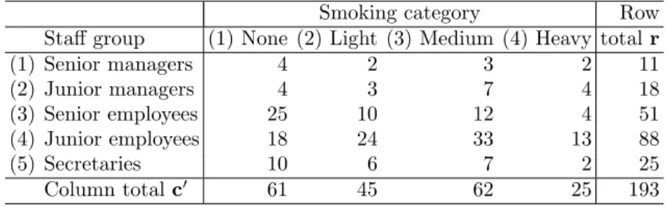
Table 1: Artificial smoking data of Greenacre (1984).The Pearson Chi-squared statistic for indepence is χ2 = 16.44.
Smoking category Row
Staff group (1) None (2) Light (3) Medium (4) Heavy totalr
(1) Senior managers 4 2 3 2 11 (2) Junior managers 4 3 7 4 18 (3) Senior employees 25 10 12 4 51 (4) Junior employees 18 24 33 13 88 (5) Secretaries 10 6 7 2 25 Column totalc0 61 45 62 25 193
2. Repeat until V does not change:
(a) Compute˜fmin and˜fmax as described above. (b) Do for all³nrnc
m
´
combinations ψ:
(c) LetCψ and dψ be the rows of Cand d defined by ψ.
• Letgψ1 be the solution of the system Cψg =
³
˜fmax−d
´
ψ
• Check if (˜fmin−d)≤Cgψ1 ≤(˜fmax−d). If so, then add gψ1 to the set of verticesV.
• Letgψ2 be the solution of the system Cψg = (˜fmin−d)ψ
• Check if (˜fmin−d)≤Cgψ2 ≤(˜fmax−d). If so, then add gψ2 to the set of verticesV.
(d) End do.
As this procedure imposes additional restrictions, the number of vertices may increase. The solution space, however, becomes smaller. Moreover, the matrices Fmin and Fmax provide us with lower and upper bounds for the integer elements of F.
7
An Illustrative Example
To illustrate our method, consider the artificial smoking data of Greenacre (1984), see Table 1.
Suppose that in addition to the marginals r and c, we have the 2-dimensional CA solution for these data. That is, in our notation, k = 3 and Rk and Ck are 5×3 and 4×3 matrices with as their first column the
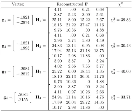
Table 2: Vertices and reconstructedFby (6) of inverse correspondence anal-ysis of the smoking data using k = 3.
Vertex ReconstructedF χ2 g1= · −.1821 −.2974 ¸ H1= 4.11 .00 6.21 0.68 3.87 5.43 3.09 5.61 25.11 8.00 15.22 2.67 18.15 21.22 37.47 11.16 9.76 10.36 .00 4.88 χ 2 1= 39.83 g2= · −.1821 .1993 ¸ H2= 4.11 .00 6.21 0.68 3.96 3.74 5.80 4.49 24.83 13.14 6.95 6.08 17.94 25.13 31.18 13.75 10.17 2.98 11.86 .00 χ 2 2= 30.43 g3= · .2084 −.2812 ¸ H3= 3.90 3.87 0 3.24 4.02 2.66 7.55 3.77 25.22 6.00 18.44 1.35 18.10 22.13 36.01 11.76 9.76 10.36 0 4.88 χ 2 3= 40.00 g4= · .2084 .2155 ¸ H4= 3.90 3.87 .00 3.24 4.11 0.97 10.26 2.66 24.94 11.14 10.16 4.76 17.89 26.04 29.72 14.35 10.17 2.98 11.86 .00 χ 2 4= 33.71
trivial solutions. We can derive U˜c and V˜c fromR0kU˜c=0 and C0kV˜c =0.
Applying the Inverse Correspondence Analysis Algorithm described in Sec-tion 4 with C=V˜c⊗U˜c and d = vec(Dr1/2RkC0kD1c/2), four valid solutions
for g are obtained. Tabel 2 contains the four vertices and the corresponding reconstructed F matrices. Thus, any convex combination of these four ver-tices yields a CA solution withRk andCk, the marginals arerandc, and the
elements of F are nonnegative. It may be verified that the convex combina-tion .1962H1+.2866H2+.2134H3+.3038H4 yields the original contingency matrix in Table 1.
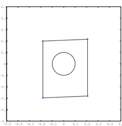
Because g only contains two elements, a visual representation of the in-verse CA solution can easily be obtained (see Figure 1). The axes represent the elements of g, that is,g1 andg2. The area inside the polyhedron is 0.194. For a g of this size, the set with λmax< λk can be graphed as circle.
For the same data, suppose that we want to impose the additional re-striction that element i = 1 and j = 4 is fixed to 2. Clearly, the problem becomes the constrained inverse CA problem. The vertices of the constrained inverse CA solution is presented in Table 3. Again it may be verified that
-0.5 -0.4 -0.3 -0.2 -0.1 0 0.1 0.2 0.3 0.4 0.5 -0.5 -0.4 -0.3 -0.2 -0.1 0 0.1 0.2 0.3 0.4 0.5
Figure 1: Polyhedron defined by inverse CA on the smoking data usingk = 3. The vertices are indicated by crosses. The dimensions are g1 and g2. The circle indicates those g that satisfy the strict inverse CA condition.
for every convex combination of the two vertices the marginals are r and c, a CA solution contains Rk and Ck, the elements of F are nonnegative, and
element i= 1 and j = 4 equals 2.
Finally, suppose it is known that the original matrix is a contingency matrix. Then, using Theorem 10 we can obtain matrices with lower and upper (integer) bounds for the values ofF. These matrices, based on the four reconstructed F matrices from Table 2, are presented in Table 4. Applying the algorithm described in Section 6.2 immediately yields one vertex g = [.0199, .0043]0, with as corresponding F matrix the original contingency
table in Table 1.
8
Conclusion and Discussion
In this paper, we have specified the set of matrices that all yield a given low dimensional configuration in its correspondence analysis solution. This set is a nonempty bounded closed polyhedron. Computing the vertices of the poly-hedron is a computationally very demanding task, even for relatively small CA problems. This task is reduced if the number of additional constraints on the elements is sufficiently large. We also specified a strict upper bound for the Pearson chi-squared statistic, not limited to inverse correspondence analysis, but also to the special case of the independence model where only the margins of the data matrix are available. Furthermore, we showed that if the data matrix is known to have integer values (as in a contingency table), then lower and upper integer bounds for the elements of the origina unknown contingency table can be obtained. In this case, the inverse CA solution set
Table 3: Vertices and reconstructed F by (6) of constrained inverse corre-spondence analysis of the smoking data using k = 3, where element i = 1 and j = 4 is fixed to 2. Vertex ReconstructedF χ2 g1= · .0199 −.2890 ¸ H1= 4.00 2.00 3.00 2.00 3.95 4.00 5.40 4.66 25.17 6.96 16.88 1.99 18.13 21.69 36.72 11.47 9.76 10.36 .00 4.88 χ 2 1= 32.56 g2= · .0199 .2077 ¸ H2= 4.00 2.00 3.00 2.00 4.04 2.31 8.11 3.54 24.88 12.11 8.61 5.40 17.91 25.60 30.42 14.06 10.17 2.98 11.86 .00 χ 2 2= 24.76
Table 4: Lower and upper bounds for the smoking data.
Lower Bounds Upper Bounds
Staff group None Light Medium Heavy None Light Medium Heavy
Senior managers 4 0 0 1 4 3 6 3
Junior managers 4 1 4 3 4 5 10 5
Senior employees 25 6 7 2 25 13 18 6
Junior employees 18 22 30 12 18 26 37 14
may be significantly reduced and can be unique.
Throughout this paper, we have assumed that the row and column marginals were known in advance together with the low dimensional CA solution. This choice can easily be justified by recognizing that the marginals can be di-rectly derived from the trivial CA dimension. However, an extension of the inverse CA problem to a situation where the marginals are unknown a priori, would lead to a much more complicated situation with a set that does not have the nice mathematical properties as in this paper.
The specification of the inverse set is available for some other multivariate analysis techniques such as multidimensional scaling (De Leeuw & Groenen, 1997; Groenen et al., 1996) and principal components analysis (Ten Berge & Kiers, 1999), or could be developed in the same spirit as the present paper. We believe that investigation of the inverse set yields better understanding of the original problem.
References
De Leeuw, J., & Groenen, P. J. F. (1997). Inverse multidimensional scaling.
Journal of Classification, 14, 3–21.
Eckart, C., & Young, G. (1936). Approximation of one matrix by another of lower rank. Psychometrika, 1, 211–218.
Gifi, A. (1990). Nonlinear multivariate analysis. Chichester: Wiley.
Greenacre, M. J. (1984). Theory and applications of correspondence analysis.
New York: Academic Press.
Groenen, P. J. F., De Leeuw, J., & Mathar, R. (1996). Least squares multidimensional scaling with transformed distances. In W. Gaul & D. Pfeifer (Eds.),Studies in classification, data analysis, and knowledge organization (p. 177-185). Berlin: Springer.
Magnus, J. R., & Neudecker, H. (1988). Matrix differential calculus with appilications in statistics and econometrics. Chichester: Wiley.
Rockafellar, R. T. (1970). Convex analysis. Princeton, NJ: Princeton Uni-versity Press.
Ten Berge, J. M. F., & Kiers, H. A. L. (1999). Retrieving the correlation ma-trix from a truncated PCA solution: The inverse principal component solution. Psychometrika, 64, 317–324.
Van de Velden, M. (2000). Topics in correspondence analysis. Amsterdam: Tinbergen Institute, University of Amsterdam.