for the k-means Problem
and Related Clustering Objectives
Dissertation
zur Erlangung des Grades eines
Doktors der Naturwissenschaften
der Technischen Universität Dortmund
an der Fakultät für Informatik
von
Melanie Schmidt
Dortmund
Dezember 2014
Gutachter: Prof. Dr. Christian Sohler, Prof. Dr. Johannes Blömer
Abstract
The continuing technological advances in different areas represent a challenge for re-searchers in computer science and in particular in the area of algorithms and theory. The gap between processing speed and data volume increases constantly, even though the per-formance of computers and their central processing units increases at a fast rate. This is because the data that surrounds us multiplies at an even more rapid pace. One example for the phenomenon is the Large Hadron Collider (CERN) that generates more than half a gigabyte of data every second. Even algorithms with linear running time are here too slow if they need random access to the data. Data stream algorithms are algorithms that only need one pass over the data to (approximately) solve a problem. Their memory usage is usually polynomial in the logarithm of the input size. Ideally, a data stream algorithm can process the data directly while it is created.
In my thesis, I consider k-means clustering. Given n points in the d-dimensional
Eu-clidean space Rd, the k-means problem is to compute k centers which minimize the sum of the squared distances of all points to their closest center. The centers can be chosen arbitrarily from Rd. For a given solution, i. e., a set of k centers, we say that the sum of the squared distances is the k-means cost of this solution. The k-means problem has been
studied for sixty years and often occurs in machine learning, also as a subproblem.
In the context of data streams, a popular technique to solve thek-means problem is the
computation of coresets. A coreset for a point setP is a (usually much smaller) point set S which has approximately the same cost as P for any possible solution. More precisely
and defined for the k-means problem, a (1 +ε)-coreset for an ε ∈ (0,1) is a set S that
satisfies that the cost ofS for any set of k centers C is at least an ε-fraction off the cost of P with the same centers C.
A coreset computation is often first designed as a polynomial algorithm with random access to the data. Then, the algorithm is converted into a data stream algorithm by using a technique which is known as Merge-and-Reduce. By using Merge-and-Reduce, the memory usage of the algorithm is usually increased by a factor which is polynomial in logn. In
joint work with Hendrik Fichtenberger, Marc Bury (né Gillé), Chris Schwiegelshohn and Christian Sohler, I developed a data stream algorithm for the k-means problem which
does not use Merge-and-Reduce. It processes the input points one by one and directly inserts them into an appropriate data structure. We use a data structure which is used in BIRCH (Zhang, Ramakrishnan, Livny, 1997), an algorithm which is very popular in practical applications. By analyzing and improving the data structure, we could develop an algorithm which computes a (1 +ε)-coreset in the data stream model and that uses
pointwise updates. Our algorithm is named BICO as a combination of BIRCH and the term coreset. The memory usage of BICO is bounded by O(k·logn·ε−(d+1)) if the dimension of the input points is a constant. We implemented a slightly modified version of BICO and combined it with an algorithm for the k-means problem which is known for its good
results in practical applications. In an experimental study, we verified that the combined implementation computes solutions with high quality while it is much faster than other implementations that compute solutions of high quality. Our work was published at the
European Symposium on Algorithms 2013.
Joint work with Dan Feldman and Christian Sohler led to an important result on thek
-means problem which was published at the ACM-SIAM Symposium on Discrete Algorithms 2013. It is a dimensionality reduction. If data is high dimensional, then reducing the dimension is as useful as reducing the number of points. We showed that it is possible to reduce the dimension of any k-means input to O(k/ε2) while preserving the cost function
up to anε-fraction. The number of dimensions is in particular independent of the number
of input points. The dimensionality reduction uses the singular value decomposition, a tool which is often used in practical applications. By combining the dimensionality result with known coreset constructions, we developed a construction that computes coresets of a size which is independent of the dimensionand of the number of input points. To achieve this,
we extended the usual coreset definition by allowing to store an additional constant. This does not increase the memory usage by much. This extension has the potential to allow for powerful coreset constructions. We develop an additional independent coreset construction for the k-means problem which also computes coresets of a size which is independent of
the dimension and number of input points. The size of the computed coresets is larger, but it is applicable to at least one additional clustering problem which can (probably) not be solved by applying the singular value decomposition.
The results described so far are the core of the first part of this thesis. The second part contains results on related objective functions, including a so-called projective clustering problem. Additionally, the second part considers a probabilistic k-median problem which
is joint work with Christiane Lammersen and Christian Sohler. The k-median problem is
defined with Euclidean distances that are not squared, other than that it is identical to the k-means problem. In the probabilistic version we assume that the input points can
appear at different locations. The probability for a point to appear at a certain location is given by a discrete probablity distribution. The task is to compute k centers that
minimize the expectedk-median cost. We develop a definition of a coreset for probabilistic
clustering and show how to compute a coreset. This result was published at the Workshop on Approximation and Online Algorithms 2012.
Zusammenfassung
Die technologischen Weiterentwicklungen in verschiedensten Bereichen bringen neue Her-ausforderungen für die Informatik und insbesondere auch für die Algorithmik und die theoretische Informatik. Obwohl Prozessorgeschwindigkeiten und rechnerinterne Kommu-nikationsgeschwindigkeiten schnell anwachsen, vergrößern sich die Datenmengen um uns herum so viel rasanter, dass Algorithmen, die man klassischerweise als effizient bezeich-nen würde, ungeeignet werden. Ein Beispiel dafür ist der Large Hadron Collider (‚Großer Hadronen-Speicherring‘, CERN), der über ein halbes Gigabyte an Daten pro Sekunde produziert. Selbst Algorithmen mit linearer Laufzeit können zu langsam sein, wenn sie wahlfreien Zugriff auf die Daten benötigen. Datenstromalgorithmen sind Algorithmen, die für die (approximative) Lösung eines Problems nur einen einzigen Durchlauf durch die gegebenen Daten benötigen, und deren Speicherplatz im Vergleich zur verarbeiteten Datenmenge sehr klein ist, üblicherweise ein Polynom im Logarithmus der Eingabegröße. Im Idealfall können Daten mit einem Datenstromalgorithmus direkt während der Entste-hung verarbeitet werden.
In meiner Dissertation beschäftige ich mich mit sogenanntemk-means Clustering, unter
anderem im Datenstrommodell. Für eine Menge von Punkten im d-dimensionalen
Euk-lidischen RaumRdist die Aufgabe,k Zentren zu finden, so dass die Summe der quadrierten Distanzen aller Punkte zu den ihnen jeweils nächsten Zentren minimiert wird. Die Zentren können dabei frei aus demRd gewählt werden. Für eine mögliche Lösung, also eine Menge von k Zentren C, bezeichnen wir die Zielfunktion im Folgenden auch alsk-means Kosten
von P mit ZentrenC. Dask-means Problem wird seit über sechzig Jahren untersucht und
tritt im maschinellen Lernen häufig auf, z.B. auch als Teilproblem.
Eine häufig verwendete Technik, um das k-means Problem im Datenstrommodell zu
lösen, ist die Berechnung von Kernmengen. Eine Kernmenge für eine Punktmenge P ist
eine (normalerweise deutlich kleinere) PunktmengeS, die approximativ für jeden möglichen
Lösungskandidaten die gleichen Kosten hat wie P. Genauer gesagt und spezifisch für das k-means Problem formuliert ist eine (1+ε)-Kernmenge für einε∈(0,1) eine Menge S, für
die die k-means Kosten von S für jede mögliche Zentrenmenge C aus k Zentren höchstens
um einen -Anteil von den k-means Kosten von P mit denselben Zentren C abweichen.
Für die Berechnung einer Kernmenge wird häufig erst ein polynomieller Algorithmus entworfen, der die Daten auch mehrfach lesen kann. Dieser wird dann mit Hilfe einer Technik, die als Merge-and-Reduce bekannt ist, in einen Datenstromalgorithmus
umge-wandelt. Dadurch erhöht sich in der Regel der Speicherbedarf um einen Faktor, der poly-nomiell in logn ist. Zusammen mit Hendrik Fichtenberger, Marc Bury (geb. Gillé), Chris
Schwiegelsohn und Christian Sohler habe ich einen Datenstromalgorithmus für dask-means
Problem entwickelt, der ohne die Merge-and-Reduce Technik auskommt. Dieser verarbeitet die Punkte im Eingabestrom einzeln und nimmt sie direkt in eine geeignete Datenstruktur. Wir verwenden eine Datenstruktur, die bereits in einem in der praktischen Anwendung sehr beliebten Algorithmus, BIRCH (Zhang, Ramakrishnan, Livny, 1997), ihre Schnelligkeit demonstriert hat. Durch eine Analyse und Weiterentwicklung dieser Datenstruktur waren wir in der Lage, einen Algorithmus zu entwickeln, der im Datenstrommodell eine (1 +ε
)-Kernmenge berechnet und nur punktweise Aktualisierungen der Datenstruktur benötigt. Der Name unseres Algorithmus ist BICO, was eine Kombination aus BIRCH und dem en-glischen Wort für Kernmenge,coreset, ist. Der Speicherbedarf von BICO ist für Eingaben
mit konstanter Dimension durchO(k·logn·ε−(d+1)) beschränkt. Wir haben BICO in einer leichten Abwandlung implementiert und mit einem Algorithmus für dask-means Problem,
der für seine guten Ergebnisse in praktischen Anwendungen bekannt ist, kombiniert. In einer experimentellen Studie konnten wir belegen, dass die kombinierte Implementierung Lösungen von hoher Qualität berechnet und sehr viel schneller ist als andere bekannte Implementierungen von Algorithmen, die Lösungen von hoher Qualität berechnen. Die Arbeit wurde auf dem European Symposium on Algorithms 2013 veröffentlicht.
Ein grundlegendes Ergebnis zum k-Means Problem ist in Zusammenarbeit mit Dan
Feldman und Christian Sohler entstanden und wurde auf dem ACM-SIAM Symposium on Algorithms 2013 veröffentlicht. Unser erstes Resultat ist eine Dimensionsreduktion. Im Falle von hochdimensionalen Daten ist es nicht nur hilfreich, die Anzahl der Punkte zu reduzieren, sondern noch viel mehr, ihre Dimension zu verkleinern. Wir zeigen, dass man die Dimension einer k-Means Eingabe aufO(k/ε2) reduzieren kann, während sich die
Zielfunktion maximal um einenε-Anteil ändert. Die Anzahl der Dimensionen ist
insbeson-dere unabhängig von der ursprünglichen Dimension. Die niedrigdimensionalen Punkte kann man mit einer Singulärwertzerlegung berechnen, ein Werkzeug, das auch in der praktischen Anwendung häufig verwendet wird. Durch eine Kombination mit vorherigen Kernmengenkonstruktionen konnten wir einen Algorithmus entwerfen, der eine Kernmenge berechnet, deren Größe unabhängig von der Anzahlund der Dimension der Eingabepunkte
ist. Wir erweitern dazu die übliche Kernmengendefinition, indem wir das Speichern einer zusätzlichen Konstanten erlauben. Dadurch entsteht kein signifikanter zusätzlicher Spe-icheraufwand. Das Potential dieser Erweiterung demonstrieren wir auch durch den Entwurf einer zweiten vollkommen unabhängigen Konstruktion für dask-means Problem, die
eben-falls eine Kernmenge mit zusätzlicher Konstante berechnet, deren Größe unabhängig von der Anzahl und Dimension der Eingabepunkte ist. Die Größe dieser Kernmenge ist größer als die aus der ersten Konstruktion, dafür lässt sich die Konstruktion auf mindestens ein anderes verwandtes Clusteringproblem übertragen, für das die Anwendung einer Singulär-wertzerlegung (wahrscheinlich) nicht möglich ist.
Die bisher beschriebenen Ergebnisse sind der Kern des ersten Teils meiner Arbeit. Im zweiten Teil beschreibe ich Ergebnisse für verwandte Zielfunktionen, unter anderem aus dem Bereich des sogenannten projektiven Clusterings. Außerdem enthält dieser Teil ein gemeinsames Resultat mit Christiane Lammersen und Christian Sohler für das probabilis-tische k-median Problem. Das k-median Problem verwendet Euklidische Distanzen, die
nicht quadriert werden, und ist ansonsten identisch zum k-means Problem. In der
proba-bilistischen Version nehmen wir an, dass die Eingabepunkte keine feste Koordinaten haben, sondern als diskrete Wahrscheinlichkeitsverteilung über mögliche Positionen gegeben sind. Das Problem ist nun, k Zentren zu berechnen, für die die erwarteten k-median Kosten
minimal sind. Wir entwickeln eine Kernmengendefinition für diesen Fall und zeigen, wie man eine Kernmenge berechnen kann. Diese Arbeit haben wir auf dem Workshop on Approximation and Online Algorithms 2012 veröffentlicht.
Acknowledgements
First of all, I would like to thank my advisor Prof. Dr. Christian Sohler from whom I have learned a lot about how to choose reseach questions and how to solve them. Thank you for advising and supporting me, for pointing me to plenty interesting research questions and for giving me the opportunity to visit summer schools and other researchers.
During the majority of my PhD time, I worked on the project ‘A practical theory for clustering algorithms’ in the DFG Priority Programme 1307 ‘Algorithm Engineering’. I thank the DFG for the funding. It was a joint project with the group of Prof. Dr. Johannes Blömer in Paderborn. I thank him and Kathrin Bujna, Dr. Daniel Kuntze and Dr. Marcel R. Ackermann for a creative environment and an enjoyable collaboration. Prof. Dr. Johannes Blömer also agreed to assess my thesis and I thank him for that, too.
I thank Marc Bury, Hendrik Fichtenberger, Dr. Martin Groß, Dr. Jan-Philipp Kapp-meier, Dr. Christiane Lammersen, Dr. Rainer Penninger, Arseny Pyatikhatka, Dr. Daniel Schmidt, Magdalena Schmidt, Chris Schwiegelshohn and Dr. Christine Zarges for proof-reading parts of my thesis. Your comments were invaluable. Special thanks go to Martin and Daniel for reading (nearly) all of my thesis and all the helpful feedback, to Jan for preparing elaborate comments despite writing his own thesis at the same time, and to Marc for checking the math in Chapter 3.
The results in this thesis are based on joint work with Marc Bury, Dr. Dan Feldman, Hendrik Fichtenberger, Dr. Christiane Lammersen, Chris Schwiegelshohn and Prof. Dr. Christian Sohler. Thank all of you for the superb collaborations.
My thanks for fruitful discussions and a nice working atmosphere go to all my colleagues in Dortmund. While writing this thesis, my colleagues helped me out to reduce the addi-tional workload, in particular Chris and Marc. Christiane always had the right words to cheer me up, both while we were working together but still when she had already left. I thank Chris, Christiane, Christine and Marc for their friendship and support. I also owe thanks for their encouragement to Dr. Thomas Jansen and Prof. Dr. Petra Mutzel.
Besides working on the content of this thesis, I had a wonderful time doing research on network flows with Daniel, Jan and Martin. Thanks belong to the three of you and to Prof. Dr. Martin Skutella and his group for welcoming us in Berlin and making this research project even more fun. Additional cooperations outside of my thesis topic were with Dr. Frank Hellweg and Dr. José Verschae. Thank you for the great time and fruitful collaboration.
I thank my parents and my sisters Katharina and Magdalena for their love and support. To my husband Daniel I owe thanks for more reasons than I can name here.
Finally, I wish to document my thankfulness to Prof. Dr. Ingo Wegener. Ingo died before I started to work on my PhD, but he is the reason why I did it. His memory accompanies me and I am very thankful for that.
1 Introduction 1
I
The
k
-means problem
5
2 Introduction to the k-means problem 7
2.1 The k-means problem . . . 10
2.2 The k-median problem . . . 17
2.3 Notations in Euclidean geometry . . . 20
2.4 A basic observation and its consequences . . . 25
2.4.1 Enumerating solutions and connections to discrete clustering . . . . 27
2.4.2 Alternative formulations fork-means . . . 28
3 Dimensionality reduction techniques 31 3.1 Two popular dimensionality reduction techniques . . . 31
3.1.1 Random projections . . . 34
3.1.2 The best fit subspace and the singular value decomposition . . . 40
3.2 The singular value decomposition revisited . . . 46
3.2.1 Weighted input sets . . . 55
4 Small coresets for the k-means problem 59 4.1 Coresets for the k-means problem . . . 59
4.1.1 Applications of strong coresets . . . 61
4.2 Techniques used in coreset constructions . . . 64
4.2.1 Moving points . . . 65
4.2.2 Uniform sampling . . . 66
4.2.3 History of coresets in view of thek-means problem . . . 70
4.3 Computing small coresets for k-means . . . 77
4.3.1 Improving the running time . . . 83
4.4 Smaller coreset sizes via dimensionality reduction . . . 85
5 The k-means problem in data streams 89 5.1 The Merge-and-Reduce technique . . . 92
5.2 Streaming algorithms for k-means clustering . . . 96
5.2.1 Algorithms based on Merge-and-Reduce . . . 96
5.2.3 Implementations of streaming algorithms fork-means . . . 99
5.3 A lower bound for BIRCH with fixed threshold . . . 102
5.4 BICO – BIRCH meets coresets for k-means clustering . . . 107
5.4.1 The basic algorithm . . . 108
5.4.2 Including rebuilding steps into BICO . . . 116
5.4.3 Running time . . . 123
5.4.4 Implementation . . . 127
5.4.5 Experimental setting . . . 129
5.4.6 Experiments . . . 131
II
Extensions of classical clustering
139
6 Kernel k-means problems 141 6.1 The k-means problem in inner product spaces . . . 1416.1.1 Coresets with offsets in inner product spaces . . . 144
6.2 The kernel k-means problem . . . 145
6.2.1 Coresets for kernel k-means problems . . . 149
7 Probabilistic k-median clustering 157 7.1 A probabilistic k-median problem . . . 160
7.2 Probabilistic coresets . . . 163
7.3 The assigned metric k-median problem . . . 167
7.4 The assigned Euclidean k-median problem . . . 171
7.4.1 Superpolynomial algorithms for the assigned Euclidean case . . . . 172
7.4.2 A coreset construction for the assigned Euclidean case . . . 174
8 Projective clustering problems 199 8.1 Introduction to projective clustering problems . . . 200
8.2 Small coresets for subspace approximation . . . 202
8.2.1 Affine subspaces . . . 203
8.3 A coreset framework for projective clustering . . . 206
8.4 The integer linear projective clustering problem . . . 209
8.4.1 Sensitivity bounds from L∞-coresets . . . 211
8.4.2 ConstructingL∞-coresets . . . 213
8.4.3 Obtaining the coreset result . . . 219
III Appendix
223
A Dissimilarity measures and vector spaces 225 A.1 Dissimilarity measures and metrics . . . 225A.3 Inner product spaces . . . 227 A.4 Sequences and Hilbert spaces . . . 228 A.5 Additional facts on Euclidean geometry . . . 229
B Additional information on BICO experiments 231
B.1 Settings . . . 231 B.2 Numerical results . . . 232
Summarizing is a natural concept. Every encyclopedia contains the population size, the gross domenstic product or the area of a country. Events are summarized in end-of-the-year reviews, books and movies are reviewed in magazines or on websites. Even this thesis contains a short summary of its contents.
We summarize data for different reasons. In a condensed form, it is easier to grasp the essentials of a topic. A summary structures data and makes it more accessible, easier to understand. The next reason is that we want to save space. In this context, summarizing means compressing. Most digital music files are stored in a compressed way to save disk space. In the context of algorithm design, there is another important aspect. Reducing the amount of input data decreases the running time of most algorithms. This is particularly true if the data is reduced to an amount that fits into the main memory, since reading data from the hard disk has significant impact on the running time. Algorithms falter because of the sheer amount of time it takes to just read the data. Lastly, there are also cases where we summarize because we simply cannot store the original data. For example, consider the data from the large hadron collidor which is so vast that it is directly filtered. Only a small fraction of the data is actually stored.
Good methods to compress data are increasingly important since we face more and more data that is automatically generated, not only from experiments in physics, but also from social media. This phenomenon has been called Big Data lately. We need new methods to compress data in a meaningful way in order to deal with terabytes and soon petabytes of data.
This thesis studies the concept of coresets. A coreset is defined in the context of an
objective function. It summarizes input data with respect to this objective function. Notice that a summary can be good for one purpose and bad for another. A summary can never be similar to the original data inevery aspect. It is sufficient if it resembles the data with
respect to the intended use. When compressing music, we want to preserve everything that the human ear can perceive. When we compress input data for an optimization problem, we want that the summary has the same properties according to the given objective function. The optimization problems studied in this thesis are geometric clustering problems.
Clustering is a summary method in its own right. It means that we partition input data into subsets of points that we believe belong together. For geometric clustering, we measure whether points belong together by similarity or dissimilarity measures. A dissimilarity measure for Euclidean points would be the Euclidean distance. Assume that we partition points into subsets such that points in the same subset are close together, and points in different subsets are far away from each other. Then we can replace each subset by a representative point and obtain a smaller data set.
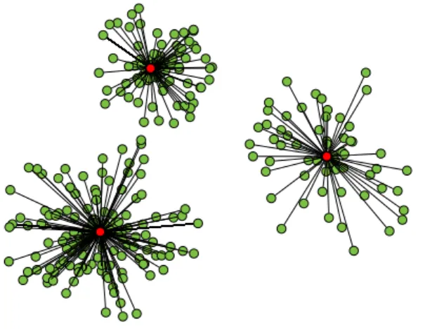
Figure 1.1: A two-dimensional input to thek-means problem and three well chosen centers.
The lines indicate which point is assigned to which center.
One of the most widely studied clustering problems is the k-means problem. It consists
of the following basic geometric question: Given a set P of points from the Euclidean
space Rd, find k centers that minimize the sum of the squared distances from every point to its closest center. A two-dimensional example for the k-means problem is depicted in
Figure 1.1. We can imagine that the centers are potential locations for new stores that a big company will open, and that they want to minimize the customer’s way to the nearest shops. Instead of shops it could also be telephone or internet exchange points, schools or public swimming baths1.
The k-means problem has the nice property that for k = 1, the solution is the centroid
of the point set, which is given by an explicit formula as the sum of the points divided by the number of points. This analytic solution to the 1-means problem implies that in an optimal solution for thek-means problem withk > 1, the input point set is partitioned into k subsets and all points in the same subset have the same center, namely the centroid of
the subset. Using this observation, thek-means problem can be solved exactly by iterating
through all partitionings of P into k subsets, computing the centroids of the subsets and
keeping track of the solution with lowest cost. Of course this algorithm is highly inefficient. In fact, it turns out that thek-means problem is NP-hard even for k = 2 [ADHP09].
The most popular algorithm for solving thek-means problem is Lloyd’s algorithm [Llo82],
a local improvement heuristic developed more than fifty years ago. Lloyd’s algorithm starts with an initial solution ofkcenters, often chosen uniformly at random from the input point
set. Then it calculates the partition induced by the center set by assigning each point to 1Intuitivelly, one might also model the above examples with non-squared distances. In this case, the
problem is called k-median problem. Both problems have many applications. The k-means problem
punishes larger distances more severely, which often makes a lot of sense: A slightly larger average way to school is certainly preferable to some children living in an insurmountable distance. We discuss differences between k-means andk-median in more detail later.
its closest cluster, thus forming k point sets. Because the optimal solution for a point
set is its centroid, the algorithm replaces the center belonging to each point set by the centroid of the point set. This can only improve the solution. The new centers induce a new partitioning, and so the algorithm iterates until convergence.
There are also various approximation algorithms known for the k-means problem, and
many of the newer algorithms are based on the computation of coresets. A coreset for the k-means problem for an input set P is a (smaller) weighted set S with the property
that for each choice of k centers, the sum of the squared distances between the points in P and the centers is approximately the same as the sum of the squared distances between
the weighted points in S and the centers. Notice that a coreset does not only preserve
the cost of an optimal or nearly optimal solution. It approximates the cost function for
every choice of centers. This is very convenient. When we run an algorithm on S, it will
behave similarly as it would when run onP. Coresets have a theoretical guarantee, in fact,
it is ensured that the cost of any solution is (1 +ε)-approximated by the coreset. Thus,
we can use coresets to speed up approximation algorithms at the expense of an additional (1 +ε)-factor in the quality guarantee.
Coresets can also be used for distributed computations or when data is given in a stream-ing settstream-ing. The latter means that the data can only be read once, in a given order that cannot be influenced by the algorithm. The constant production of data by the large hadron collidor is a prime example for a streaming setting. The algorithm cannot store all of the data but only a small fraction of it.
The topic of this thesis is the study of coresets and related summaries. The thesis has two parts. The first part is devoted to the k-means problem, while the second part discusses
additional clustering objectives.
Chapter 2 introduces the k-means problem, gives a brief outline of its history, its
ap-proximability, and its complexity. The k-median problem, which is closely related to the k-means problem, is also introduced. Furthermore, the chapter contains a short
intro-duction to Euclidean geometry and basic techniques for the development of algorithms in the context of the k-means problem.
Chapter 3 addresses dimensionality reductions for the k-means problem. If data is high
dimensional, summarizing it can also mean that we reduce the dimension instead of the number of points. The chapter contains a review of methods that reduce the dimension of the points but preserve the k-means objective function up to a factor of (1 +ε). Then,
a new method is presented that is able to reduce the dimension of an input point set to
O(k/ε2) while the k-means objective is changed by at most anε-faction.
Chapter 4 introduces coresets for thek-means problem, reviews their history and known
coreset results. Additionally, two important methods to construct coresets are discussed. One of them is sampling. The chapter concludes with two new coreset constructions. Both
have the property that the number of points in the coreset is independent of the number of input points and it is also independent of the dimension of the input points.
Chapter 5 discusses the computation of coresets in data streams. It starts with an
introduction to the streaming setting and explains the Merge-and-Reduce technique which can be used to embed coreset constructions into streaming. Then, existing streaming algorithms for the k-means problem are reviewed, and one of the coreset constructions
from Chapter 4 is embedded into Merge-and-Reduce. The chapter concludes with the presentation of BICO, a coreset construction for the k-means problem in the streaming
setting which has a theoretical guarantee but is also easy to implement and fast in praxis.
Chapter 6 is the first chapter of the second part of the thesis. It considers the kernel
k-means problem which is a generalization of thek-means problem for instances that are
not linearly separable. One of the constructions from Chapter 4 is observed to work in so called inner product spaces. This insight is then used to construct coresets for the kernel
k-means problem.
Chapter 7 considers a probabilistic clustering problem. Here, points can appear at
dif-ferent positions within a given metric space. Coresets are constructed for a probabilistic
k-median problem, both in the Euclidean space and in finite metric spaces. The chapter
also contains approximation results for both problems.
Chapter 8 introduces projective clustering problems. This generalization is the task to
cluster points with affine subspaces. Notice that points are affine subspaces of dimension zero. A coreset construction for clustering with one j-dimensional subspace is presented,
followed by a coreset construction for clustering with k subspaces of dimension j.
The results in this thesis arose from collaborations with Marc Bury, Dan Feldman, Hen-drik Fichtenberger, Christiane Lammersen, Chris Schwiegelshohn and Christian Sohler. Chapters and sections which present original research refer to the publications and name the co-authors. For all publications with n authors, I have contributed at least 1/n of the
Clustering is an old1 and broad topic and the term itself is hard to define concisely. Jain [Jai10] states that the goal of clustering is ‘to discover the natural grouping(s) of
a set of patterns, points or objects’ and that the aim of cluster analysis is to find an ‘auto-matic algorithm’ to do so. This statement describes the inherent motivation of clustering, and it tells us that a clustering partitions an input into subsets, also called clusters.
Clustering is an unsupervised method, meaning that it tries to ‘discover’ the structure
hidden in the data without external guidance. This differentiates clustering from supervised learning methods, where parts of the data include class labels.
Given Jain’s broad notion of clustering, it is natural that clustering has applications in many very different areas. Indeed, Jain [Jai10] names image segmentation / computer vision, information access and retrieval, grouping customers for efficient marketing, work-force management and planning, and the study of genome data in biology as examples. We can imagine that clustering plays a role whenever objects shall be grouped into similarly behaving subgroups, whenever structure is searched for in not yet understood data, and whenever large data sets need to be compressed into a set of meaningful representatives.
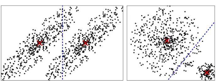
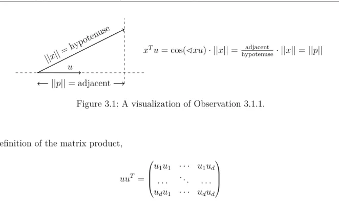
The different application areas also mean that there is not ‘the’ clustering method. Consider Figure 2.1 which shows an example by Jain (approximately reproduced from [Jai10]). Jain uses it as a visualization of different cluster shapes and densities and states that ‘Although these clusters are apparent to a data analyst, none of the available clustering algorithms can detect all these clusters.’
Even more, we notice that this example also illustrates that the ‘natural’ clustering (and thus, the right choice of the clustering objective) often lies in the eye of the beholder. Depending on the application and the overall structure of the data, we might well consider the orange, gray and purple cluster as one cluster. Consider Figure 2.2 which shows two point sets including these these three sets in a different context. In the right picture of Figure 2.2 we would probably indeed identify these three point sets as different clusters. However, in the left picture we might favour to see them as one cluster.
Because of the large number of different applications and thus also large number of different goals, various clustering problems and algorithms exist in the literature. Several 1Hansen and Jaumard [HJ97] claim that clustering dates back to Aristotle. In fact, in his text
‘Cate-gories’ [Ari], Aristotle derives ten categories to classify objects and concepts, which shows an under-standing of the concept of partitioning options due to their properties. Additionally, the Stanford Encyclopedia of Philosophy [Len11] also names Aristotle the ‘originator of the scientific study of life’ because ‘his zoological writings provide a theoretical defense of the proper method for biological inves-tigation; and they provide a record of the first systematic and comprehensive study of animals’, which is based on several of his other writings. While discussing whether Aristotle really worked on clustering is besides the point, we conclude that the desire to classify and categorize is indeed an old one.
Figure 2.1: Example reproduced after Figure 2 in [Jai10]. The left side presents the input. In the right picture, the points are colored according to the desired clustering.
Figure 2.2: Two examples including the orange, gray and purple cluster from Figure 2.1.
surveys and books have been written to summarize and classify the different approaches. These include earlier books by Anderberg [And73] in 1973, by Hartigan [Har75] in 1975 and by Jain and Dubes [JD88] in 1988, newer publications like the review by Jain, Murty and Flynn [JMF99] in 1999 or the book by Everitt, Landau and Leese [ELL09] (first edition 2001), and even more recent publications by Xu and Wunsch [XW05] in 2005, Berkhin [Ber06] in 2006 or the data clustering survey by Jain [Jai10] in 2010. The latter survey has already been cited more than 850 times (according to Google Scholar [Goo14], accessed on 31st of January 2014)2, which highlights the popularity of the topic even more. While there is no commonly agreed upon specification, introductions to the field usually ask of a clustering that objects are only grouped together if they are in some way similar. For example, Berkhin [Ber06] says that ‘clustering is a division of data into groups of similar objects’. Often, it is also required that objects that are not grouped together
and are thus classified as different, are in some way dissimilar. Xu and Wunsch [XW05] write that ‘most researchers describe clusters by considering the internal homogeneity and the external separation.’ However, these goals might be hard to achieve simultaneously. The definition currently found on the online encyclopedia Wikipedia [Wik] gives a slight relaxation by demanding of a clustering that ‘objects in the same group (called a cluster) are more similar (in some sense or another) to each other than to those in other groups (clusters).’ For our purposes, we will keep the following stability-type idea in mind: A clustering is a partitioning of a set of objects into clusters such that every object satisfies that it is in some way more similar to the objects in its cluster than to the objects in other clusters.
There are various ways to specify what we mean by similar, and this depends on the application area. For example, assume we want to cluster strings of a fixed length from a finite alphabet. Then the similarity between two strings could be measured by the number of coinciding characters. If we normalize the similarity measure by dividing by the string lengths and consider binary strings, this measure is called (simple) matching coefficient (see for example Everitt, Landau, Leese [ELL09]). Yet, there are several other similarity measures for binary strings, and following the presentation in [ELL09], we see that this is due to different application areas. The expressiveness of a match can be low if the bit encodes the presence of something rare, for example a rare genetic defect. If the match encodes the absence of this defect, then it is disputable whether this really indicates a significant similarity. So, depending on the actual scenario, different measures are reasonable, and [ELL09] lists six different relatively simple similarity measures for binary strings alone.
Often, dissimilarity measures provide a more natural modelling. If the objects are
co-ordinates on a city map, then we probably associate similarity with closeness, or, in other words, low dissimilarity. As for similarity measures, there are several ways to define dis-similarities, even if we fix an underlying metric like the Euclidean distance measure. In the introduction, we already got to know the k-means problem, where the dissimilarity of
points in the Euclidean space is measured by the Euclidian distance, but squared. This is a very common modelling, and the remainder of this chapter is devoted to the introduction to this problem. In Section 2.2, we look at the k-median problem, the close relative of
the k-means problem where the distances are non-squared. Other dissimilarity measures
related to the Euclidean space include lq
p distances which are based on the q-th power of
p-norms3 and Mahalanobis distances4.
Before we now take a closer look at thek-means problem, one final remark regarding the
type of clustering that is done in this thesis. The clustering algorithms in this thesis belong to the field ofpartitionalclustering. This means that they look for partitionings of the input
data into subsets in a way that optimizes a clustering objective function. For example, algorithms for the k-means or k-median problem can be viewed as partitional clustering
3Thelq
p distance of two pointsx= (x1, . . . , xd)T andy= (y1, . . . , yd)T from Rd is
Pd
i=1|xi−yi|
pq/p.
4For a symmetric positive definite matrix A
∈ Rd×d, the corresponding Mahalanobis distance of two
pointsxandy fromRd isp
algorithms. Every solution (a set of k centers) induces a partitioning (by assigning every
point to its closest center) with a certain cost (the sum of the [squared] distances of all points to their centers). This cost is then optimized.
The wide field of clustering contains other approaches as well. For a systematic overview on different approaches and viewpoints, see for example [Ber06] and [JD88]. One popular example is hierarchical clustering. Hierarchical clustering computes a nested sequence of
partitions, i. e., the input point set is subsequently subdivided, usually until a level where all subsets are singletons (only contain one point). The subdivision is done according to a splitting criterion based on similarity. A hierarchical clustering algorithm can also start with the set of singletons and subsequently merge these based on a similarity merging criterion. Our only brief contact with hierarchical clustering will be in Chapter 5.3 because the algorithm BIRCH described there uses a hierarchical clustering algorithm.
2.1 The
k
-means problem
Now, we consider the objective function on which the ‘most commonly used partitional clustering strategy’ [JD88] is based upon. Thek-means objective function seeks to minimize
the sum of the squared distances of all points to a set of k centers. It is also known as
square error criterion or sum of squared errors, usually abbreviated by SSE.
The squared Euclidean distance is an old clustering objective. Bock [Boc07] traces the
k-means problem back to 1950 to a paper by Dalenius [Dal50]. The still most popular
algorithm for the k-means problem was already developed in 1956 by Steinhaus [Ste56]
and independently in 1957 by Lloyd [Llo57]. The immense popularity of the k-means cost
function becomes most apparent in the popularity of this algorithm. We discuss it below. The k-means problem is specified with adissimilarity measure, the Euclidean distance.
We will review the definitions and notations in Euclidean geometry below, for now it is only important that we denote the Euclidean space by Rd and the Euclidean norm by|| · ||. In addition to thek-means objective function, we also define thek-median objective function.
Firstly, we will consider (a probabilistic version of) the k-median problem in Chapter 7.
Secondly, we will occasionally use the k-median problem for comparisons of properties of
the k-means problem. We also define a popular variant of both problems, called discrete
clustering.
Definition 2.1.1 (k-means and k-median). Let P ⊂ Rd be a finite set of points in the
d-dimensional Euclidean space, let k ∈ N be positive integer. The (Euclidean) k-median problem is to find a set C ⊂Rd of k points (called centers) that minimizes the sum of the
Euclidean distances of the points in P to their closest center in C, P
x∈P minc∈C||x−c||.
The (Euclidean) k-means problem is to find a set C ⊂Rd of k points that minimizes X
x∈P min
c∈C ||x−c|| 2,
Figure 2.3: Examples of point sets that are to be partitioned into two clusters. The red points are chosen to lie at the center of the intuitive clusters. The blue lines show the partitioning created by assigning each point to its closest center. This partitioning is probably not the intuitive one.
If the point set is weighted by a function w : P → R, the weighted k-means problem is
the task to minimize P
p∈P minc∈Cw(x)||x−c||2 over the choice of C ⊂ Rd with |C| =k.
Thediscrete(possibly weighted) Euclideank-means ork-median problem is verbatim except that it does not optimize over C ⊂ Rd, but over all choices of C from a finite set, e. g.,
from the input point set.
Notice that discrete clustering problems are discrete with respect to the set of centers, not with respect to the input point set. Standard discrete clustering problems use the input point set as the candidate set for the centers. So, if we talk about ‘the’ discrete
k-means ork-median problem, we mean that the candidate set is equal to the input point
set. Complementary to the discrete case, k-means and k-median problems withRd as the candidate space for the centers are also refered to as continuous.
For all these problems, we also call the value of the objective function thecost ofP with
a given center set C or theoptimal cost of P for the optimal choice ofC.
Limitations for finding ‘natural’ clusterings. As we discussed above, no (known)
clus-tering objective finds every ‘natural’ clusclus-tering. The k-means objective is particularly
well-suited for spherical clusters with relatively equal radii. Figure 2.3 shows two examples where with the ‘natural’ centers, the implicit assignment of points to centers does not lead to the natural clustering. Notice however that both examples show clusters which are very close together compared to their radii. If the clusters are well-spread, an optimal k-means
clustering is more likely to coincide with the intuitively expected result.
Additionally, consider Figure 2.2. While the four clusters in the picture on the left side may be found with an algorithm for thek-means problem, the seven clusters in the picture
they are not linearly separable – there is no way to define centers that partition the two-dimensional space into rings. In Section 6.2, we will see an extension of k-means designed
for this type of data.
Finally, notice that for optimizing thek-means clustering function, the value of k must
be known in advance, or, if we want to find it (for example by binary search), an additional quality measure of the resulting clustering is needed. The k-means objective is
monoton-ically decreasing in the number of clusters. Many approaches exist to determine a good number of clusters. Section 5 in the paper by Tibshirani, Walther, and Hastie [TWH01] and the summary by Gordon [Gor96] can serve as a starting point. One idea is to look for a significant drop in the cost followed by a relatively stable cost (the elbow method).
So if there exists a number of centers k where the optimal k-means cost drops
unpropor-tionally compared to the optimal (k−1)-means cost, but does not continue to decrease
significantly when considering k+ 1 optimal centers, the ‘right’ number of clusters might
have been found.
Lloyd’s algorithm. The most popular algorithm for the k-means problem is Lloyd’s
algo-rithm. It is a local improvement strategy. Starting with an arbitrary solution consisting of
k centers from Rd, two steps are iterated until convergence is reached or until a stopping criterion is satisfied. First, every input point is assigned to its closest center, ties broken arbitrarily. This results in a partitioning of the point set into k clusters. Second, the
optimal 1-means solution is computed for each subset in this partitioning. The optimal solution fork = 1 is the centroid (which is the sum of the points divided by their number),
so the 1-means solutions for the k subsets can be computed in time O(ndk). The centers
are then replaced by the k centroids and the algorithm continues with these new centers.
When we consider the sum of the squared distances of all points to the center that they are assigned to, both steps can only decrease this sum. To see this, notice that computing the centroids while keeping the partitioning can only decrease the cost because the centroid is the best 1-means solution. Reassigning the points to their now closest center can again only decrease the cost. There are only finitely many ways how a point set of n points
can be partitioned, thus the algorithm will eventually converge to a situation where the reassignment of the points results in the same partitioning as before. Then, the algorithm stops.
Due to its popularity, Lloyd’s algorithm is actually often calledk-means algorithm. We
avoid this naming because the term was first used by MacQueen [Mac67] to name a differ-ent algorithm for thek-means problem, causing some potential for confusion, and because
the reference to Lloyd is also common. The algorithm was, however, independently dis-covered by Steinhaus [Ste56] even before Lloyd described it in 1957 [Llo57]. According to Bock [Boc07], referring to Lloyd is common in ‘computer science and pattern recognition communities’. Both Steinhaus and Lloyd actually considered a continuous version of thek
-means problem and thus also of the algorithm. According to Bock, the first to propose the discrete algorithm was Forgy as part of a lecture which is documented in other publications (the usual reference [For65] is the abstract of this talk).
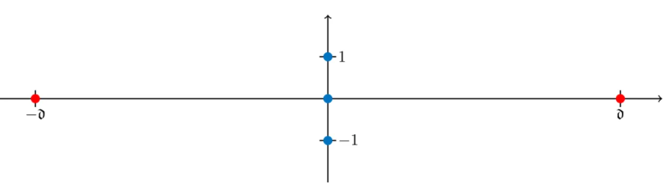
−1
1
−d d
Figure 2.4: An example with five points where the blue points form a local but not global optimum fork = 3.
Lloyd’s algorithm is over fifty years old. It is probably indeed ‘the best-known’ algorithm for thek-means problem as Xu and Wunsch [XW05] call it, has been titled ‘the most
com-monly used partitional clustering strategy’ [JD88] and the ‘by far most popular clustering tool used in scientific and industrial applications’ [Ber06]. The recent survey by Jain [Jai10] again certifies that ‘it is still one of the most widely used algorithms for clustering’, despite its age. Lloyd’s algorithm was also named one of the ten most influential algorithms in the data mining community after a three-stage recommendation process by the organiz-ers of the IEEE International Conference on Data Mining (ICDM), as documented in the publication by Wu et. al. [WKQ+08].
The enormous popularity of Lloyd’s algorithm might be due to its simplicity (both steps are easy to understand and implement) and the experience that it is often fast (if we simply stop after running a constant number of iterations, the running time is O(nkd)) while
computing reasonable solutions, or because of the lack of an always convincing alternative, as Jain [Jai10] implies.
However, the algorithm does not come with a polynomial running time guarantee or a guarantee on the quality of computed solutions. After Dasgupta [Das03] and Har-Peled and Sadri [HPS05] raised the question on the running time of Lloyd’s algorithm and gave first bounds, Arthur and Vassilvitksii [AV06] and Vattani [Vat11] showed that the number of necessary iterations can be exponential in the number of points, and this can even happen for points in R2.
When the algorithm converges, the result is a local optimum, but it is not guaranteed to be a global optimum or an approximation of one. Figure 2.4 depicts a five point example for this described by Mettu and Plaxton [MP04]. The coordinates of the blue points are (0,−1), (0,0) and (0,1), the coordinates of the red points are (−d,0) and (d,0). If Lloyd’s
algorithm is initialized with the blue points, then assigning every point to its closest centers and computing the centers again yields the blue points as centers. The optimal solution would be to pick (−d,0), (0,0) and (d,0) as centers, which costs 2. The local optimum has
The k-means++ algorithm. As already apparent in the above example, the initialization of Lloyd’s algorithm is crucial for the quality of the solution. Among the many methods to find good initial centers, we discuss one method in more detail. In 2009, Arthur and Vassilvitskii [AV07] proposed the algorithm k-means++, which consists of a clever random
initialization process followd by Lloyd’s algorithm. The centers are chosen iteratively. The first one is drawn uniformly at random from the point set. In each of the remaining k−1
steps, the centers are chosen according to a probability function based on the current cost of the points. More precisely, the probability to choose a point is the squared distance to its closest center divided by the sum of the squared distances of all points to their closest center. The intuitive idea behind this procedure is to choose points which have a high cost in the current solution. If a cluster of points lies very far away from any so far chosen center, it is probably a good idea to pick one of its points. The same holds if a cluster is only medium far, but contains a lot of points. By choosing the probability distribution based on the current cost of the points, both of these scenarios are covered at the same time (in contrast to for example simply picking the currently most expensive point).
Arthur and Vassilvitskii show that the k centers chosen by this random procedure are
themselves a O(logk)-approximative solution. Applying Lloyd’s algorithm enhances the
solution further, providing a local optimum of at least the same quality.
The distinctive feature ofk-means++ is that it is an easy algorithm and practically fast,
but it comes with an approximation guarantee, even though this guarantee is high.
Complexity of the k-means problem. As the popularity of a potentially exponential
algorithm already indicates, thek-means problem is NP-hard. It has two parameters, and
it is a natural approach to check whether fixing these to constants influences the hardness of the problem. The parameters are the number of centersk and the dimensiondof the input
points. We might ask if fixing one of them and applying some sort of enumeration strategy can yield a polynomial algorithm. Notice that we cannot easily enumerate all possible centers as there are infinitely many possibilities. In Section 2.4, we see that the 1-means problem can be solved analytically. We also see that this implies that we can solve the
k-means problem by iterating through all partitions of the input point set, computing the
1-mean of every subset and keeping track of the best solution. However, this enumeration algorithm is not polynomial, not even for constant k. In fact, if the dimension of the
problem is arbitrary, then the k-means problem is NP-hard even for k = 2. A short proof
for this is due to Aloise, Deshpande, Hansen and Popat [ADHP09], a proof containing a sequence of reductions is due to Dasgupta [Das08]. The motivation for their work was an error in a previous proof due to Dasgupta, Frieze, Kannan and Vempala [DFK+04]. The k-means problem is also NP-hard for constant dimension and arbitrary k by the work
of Mahajan, Nimbhorkar, and Varadarajan [MNV09], more precisely, even for d = 2.
For constant dimension and a constant number of centers, the problem can be solved in polynomial time by the algorithm of Inaba, Katoh, and Imai [IKI94]. It is indeed an enumeration algorithm, iterating through all possible partitions which can be induced by weighted Voronoi diagrams.
Authors Year Guarantee Running Time Reference
k and dare arbitrary
Jain, Vazirani 1999 ≤108 poly(n, d, k) [JV01]
Kanungo, Mount, Netanyahu, Piatko, Silverman, Wu
2002 O(1) poly(n, d, k) [KMN+04]
Mettu, Plaxton 2002 O(1) O(ndk) for
polyno-mial coordinates and
k∈[logn, n/logn]
[MP04] Arthur, Vassilvitskii 2007 exp. O(logk) O(ndk) [AV07]
Aggarwal, Deshpande,
Kannan 2009 O(1) O(ndk) + poly(k,logn) [ADK09]
k is arbitrary,dis a constant Kanungo, Mount, Netanyahu, Piatko, Silverman, Wu 2002 9 +ε ω(nε−dln 1/ε) [KMN+04] k is a constant,dis arbitrary
Drineas, Frieze,
Kan-nan, Vempala, Vinay 1999 2 O(n
k3/2) + poly(d, n) [DFK+04] Ostrovsky, Rabani 2000 1 +ε O(n(k+ε−1)O(1)) [OR02]
de la Vega, Karpinski,
Kenyon, Rabani 2003 1 +ε O(n(log
kn) · ε−8lnε−1),
precomputed distances [dlVKKR03] Kumar, Sabharwal, Sen 2004 1 +ε O(nd·2(k/ε)O(1)) [KSS10]
Chen 2006 1 +ε O(nd+ 2(k/ε)O(1)d2logk+2n) [Che09]
Feldman,
Monemizadeh, Sohler 2007 1 +ε O(nd)+d·poly(1/ε)+2 ˜
O(k/ε) [FMS07] Feldman, Langberg 2011 1 +ε O(nd+ 2poly(1/ε,k)) [FL11b]
Jaiswal, Kumar, Sen 2012 1 +ε O(nd·2O˜(k2/ε)) [JKS14] k is a constant, dis a constant
Hasegawa, Imai, Inaba,
Katoh 1993 2 O(n
k+1) [HIIK93]
Inaba, Katoh, Imai 1994 1 nO(dk) [IKI94]
Matoušek 2000 1 +ε O(nlogknε−2k2d) [Mat00]
Har-Peled, Mazumdar 2004 1 +ε O(n + log9n + ε−(2d+1)klogk+1nlogk(1/ε))
[HPM04] Effros, Schulman 2004 1 +ε (1/ε)O(d)nlog logn +
(1/ε)O(kd)
[ES04] Frahling, Sohler 2005 1 +ε O˜(nlog3∆ + log9n +
ε(−2d+1)k)
[FS05] Har-Peled, Kushal 2005 1 +ε O(n + poly(logn,1/ε)
+f(ε))
[HPK07]
The NP-hardness naturally raises the question whether approximation algorithms ex-ist. To the best knowledge of the author of this thesis, the status of current reseach is the following. For constant k and constant d, the problem is polynomially solvable and
polynomial approximation schemes serve only to speed up the running time. Matoušek was the first to propose such a PTAS in [Mat00]. Constructing a PTAS is still possible for arbitrarydand constantk, and the first PTAS in this scenario was given by Ostrovsky and
Rabani [OR02]. In this case, even linear time (1 +ε)-approximation schemes are possible,
and the first such scheme was given by Kumar, Sabharwal and Sen [KSS10].
Ifk is arbitrary, no (1 +ε)-approximation is known, not even for constant dimension. It
is also not known whether the problem is APX-hard. Constant approximations are pos-sible, even if k and d are variable. The first such approximation was given by Jain and
Vazirani [JV01] who proposed a primal-dual algorithm for the k-median problem which
can be extended to the k-means problem. They give 108 as a rough upper bound on the
approximation guarantee, but state that a much better guarantee is achievable. Kanungo, Mount, Netanyahu, Piatko, Silverman and Wu [KMN+04] propose an approximation based on a local search algorithm proposed in [AGK+04] for the k-median problem. Their algo-rithm can be used in two ways. In a basic version, it achieves an approximation a little better than Jain and Vazirani, but is also applicable in the scenario of variabled andk. In
a refined version, the approximation guarantee is improved to 9 +ε, but the running time
is only polynomial for constant dimension d. However, a slight change to the algorithm
most likely reduces the running time to be polynomial in d, too.
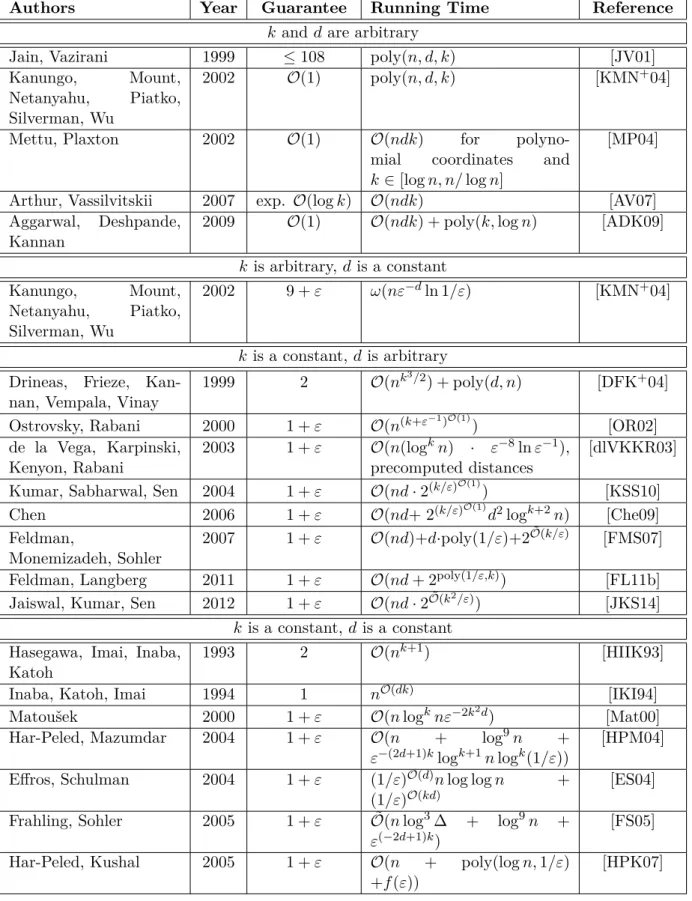
Table 2.1 gives an overview including many important steps in the development of faster
k-means approximation algorithms. It is meant as a (probably not complete) look-up table
for different approximation algorithms, giving an impression of the variety of available approximation algorithms for the k-means problem.
Remarks on Table 2.1. Notice that the algorithm by Inaba, Katoh and Imai [IKI94] is
deterministic, but most of the cited algorithms are randomized. In this case, the running times are stated under the assumption that random numbers can be drawn in O(1).
Gen-erally, the running times do not include terms which are assumed to be constant. The algorithms developed in [Che09, FS05, FMS07, FL11a, HPM04, HPK07] involve the de-velopment of coresets and were designed for data streaming settings. We discuss coresets in Chapter 4, and data streams in Chapter 5.
The algorithm by Frahling and Sohler [FS05] was developed forgeometric data streams,
where the assumption is that the input points lie on the grid {1, . . . ,∆}d for a constant ∆. Such a grid can always be found by scaling and translating the points, then ∆ has to be at least the spread of the input point set, i. e., the quotient of the maximum and minimum distance of all input points.
The algorithms by Jain and Varadarajan [JV01] and Mettu and Plaxton [MP04] were originally developed for thek-median problem but were later noted to work for thek-means
problem, too.
[AV07]. It is definitely exponential in d because it uses a so-called centroid set due to
Matoušek [Mat00] as a candidate set for centers instead of using Rd. This induces only a (1 +ε)-error. Using the algorithm without the centroid set and instead using P as the
candidate set for centers induces a higher approximation ratio, but yields an algorithm with polynomial dependence on d. For a more detailed analysis of such a version of the
local search algorithm, also see [SR10], where an upper bound of 50 for the approximation guarantee is given.
The approximation guarantee of the algorithm by Arthur and Vassilvitskii [AV07] is on expectation, so a single run of the algorithm may return a worse result.
The table only lists results that were explicitly stated for the k-means problem and
are not bicriteria approximations. Notable additional results include the generic sampling algorithm that can be used to speed up approximation algorithms and was analyzed by Mishra, Oblinger and Pitt [MOP01] and later by Czumaj and Sohler [CS04], and which is one basis of the algorithm by [Che09]. We discuss it in more detail on page 72 in Section 4.2.3.
Organization of the remainder of this chapter. In Section 2.2, we shortly review results
on the very related k-median problem. After that, we look at useful observations that help
solving the k-means problem. Our choices are subjective and motivated by the topics
that are considered in later chapters. Section 2.3 could also be titled ‘Preliminaries’ as it contains definitions and notations that are later needed. In Section 2.4, we introduce a ‘folklore’ finding from linear algebra. Despite its simplicity, it has had a huge impact on the study of the k-means problem and on the design of algorithms for it. We also see a
few of its direct consequences.
2.2 The
k
-median problem
We consider the two most common k-median problems. For us, ‘the’ Euclidean k-median
problem is the task to compute k centers from Rd such that the sum of the non-squared distances from each input point to its closest center is minimized. It is closely related to the k-means problem.
For thek-median problem, it is also very common to consider finite metric spaces, i. e.,
a set X with a distance function d: X×X →R+ that satisfies the triangle inequality, is
non-negative and symmetric (andd(x, y) is only zero iffx=y). We formally define metrics
in Section A.1. For k-median problems in finite metric spaces, the input point set P ⊂X
is a subset of the metric space. By ‘the’ metric k-median problem we mean the problem
to compute k centers from P that minimize the sum of the distances of all points in P to
its closest center. So, centers can only be chosen from the input point set.
Both versions are well-studied, and they are quite related to the k-means problem.
The k-means counterparts of some of the results discussed below are also mentioned in
Authors Year Guarantee Running Time Reference Bartal 1996 O(klognlogkn) poly(n, k) [Bar96]
Bartal 1998 O(lognlog logn) poly(n, k) [Bar98]
Charikar, Chekuri, Goel, Guha 1998 O(logklog logk) poly(n, k) [CCGG98]
Charikar, Guha, Tardos,
Shmoys 1999 6
2
3 poly(n, k) [CGTS02]
Jain, Vazirani 1999 6 O˜(n2) [JV01]
Charikar, Guha 1999 4 O˜(n3) [CG05]
Arya, Garg, Khandekar,
Meyer-son, Munagala, Pandit 2001 3 +ε poly(n, k) [AGK +04] Guha, Meyerson, Mishra,
Mot-wani, O’Calaghan 2000 O(1)
˜
O(nk) [GMM+03]
Mettu, Plaxton 2002 O(1) O(nk) for k ∈
[logn, n/logn]
[MP04] Charikar, O’Callaghan,
Pani-grahy 2003 O(1) one-pass stream-ing algorithm [COP03]
Chen 2006 10 +ε O(nk +
k7ε−5log5n)
[Che09] Li, Svensson 2013 1 +√3 +ε O(nε−2) [LS13]
Table 2.2: Some approximation algorithms for the metric k-median problem.
Complexity. The metrick-median problem is NP-hard [KH79b]. The Euclideank-median
problem is also NP-hard, even in the plane [MS84]. The variant where the centers can only be chosen from the input points (but the metric space is the Euclidean space) is also NP-hard, as shown by Papadimitriou [Pap81]. Additionally, the Euclideank-median problem is
the Fermat-Weber problem fork = 1. As we mentioned before, the Fermat-Weber problem
cannot be solved optimally by an algorithm that uses only arithmetic operations and the computation of roots [Baj88].
Notice that the metrick-median problem can be solved in polynomial time by iterating
through all possibilities to choose k centers fromn input points if k is constant.
Approximation algorithms for the metric k-median problem. For the metrick-median
problem, no PTAS is known for the case of arbitrary k, and most likely, none exists. Lin
and Vitter [LV92] showed that computing a (1 +ε)-approximation to the metrick-median
problem is NP-hard. Guha [Guh00] showed that it cannot be approximated within a factor less than 1 + 1/e unless it holds that NP⊆DTIME[nO(log logn)]. The bound was improved by Jain, Mahdian and Saberi [JMS02]. They showed that the metric k-median problem
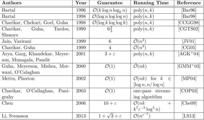
cannot be approximated within a factor less than 1+2/eunless NP⊆DTIME[nO(log logn)]. Table 2.2 gives an overview on some approximation algorithms for the metrick-median
problem. The approximation guarantee has been continuously improved. Two particu-larly noteworthy contributions are the first constant-factor approximation due to Charikar,
Guha, Tardos and Shmoys [CGTS02] and the algorithm with the currently best approxi-mation ratio due to Li and Svensson [LS13], which was developed after a rather long period without an improvement of the best known approximation ratio. The ratio is 1 +√3 +ε.
We notice two details. First, the constant approximation due to Chen [Che09] uses coresets. The coreset size istO(dk2−2lognlog(k/ε)). Second, Mettu and Plaxton [MP04]
developed not only an algorithm but also proved an Ω(nk) lower bound on the running
time of any constant-factor approximation, even for randomized algorithms, which is nearly matched by their running time and the running time of the algorithm due to Chen.
In addition to approximation algorithms like in Table 2.2, there exist several algorithms that compute approximations under relaxed conditions, for example bicriteria approxima-tions which relax the number of centers. For example, a randomized bicriteria approxi-mation by Indyk [Ind99], which is of particular interest to us, computes O(k) centers that
provide a constant factor approximation. The running time is ˜O(nk/δ2) where δ is the
failure probability of the algorithm. Another example is an algorithm due to Meyerson, O’Callaghan and Plotkin [MOP04]. It is a constant factor approximation with running time
˜
O(k((k2/ε)·logk)2) under the assumption that there exists an optimal solution where each
cluster has at least Ω(nε/k) points for a constant ε >0.
The algorithms by Guha, Meyerson, Mishra, Motwani and O’Callaghan [GMM+03] and by Charikar, O’Callaghan and Panigrahy [COP03] work in the streaming model. The algorithm in [GMM+03] needs O(nε) space and computes a 2O(1/ε)-approximation. The algorithm in [COP03] needs O(klog2n) space.
Approximation algorithms for the Euclidean k-median problem. When the set of
can-didates is restricted to the input point set, then the Euclideank-median problem is a special
case of the metrick-median problem. By the triangle inequality, optimally solving this
dis-crete version yields a 2-approximation for the Euclidean k-median problem where centers
can be chosen from Rd. Consequently, all approximation algorithms in Table 2.2 induce constant approximations for the Euclidean k-median problem with twice the constant.
When either k or d is constant, then the (continuous as well as the discrete)
Eu-clidean k-median problem can be approximated to arbitrary precision. Table 2.3 lists
(1 +ε)-approximations for the Euclidean k-median problem for either constant d or k.
The first (1 +ε)-approximation algorithm is due to Arora, Raghavan and Rao [ARR98].
It is based on the famous result due to Arora [Aro98] on the Euclidean Traveling Salesman problem and works for instances in the Euclidean plane, so the dimension is a constant. Kolliopoulos and Rao [KR07] developed the first (1 +ε)-approximation that works in Rd for constant dimensions d ≥ 2, but for the discrete version of the problem. Nevertheless,
it is the base algorithm used by the coreset based results for constant d.
For constant k, the first PTAS is due to Ostrovsky and Rabani [OR02], followed by the
paper that introduced coresets to clustering and which is due to Bădoiu, Har-Peled and Indyk [BHPI02]. The base algorithm for the coreset construction due to Chen [Che09] and Feldman and Langberg [FL11a] is due to Kumar, Sabharwal and Sen [KSS10]. The algorithm by Feldman, Monemizadeh and Sohler [FMS07] is stated to be extendable to
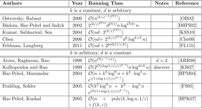
Authors Year Running Time Notes Reference
k is a constant,dis arbitrary
Ostrovsky, Rabani 2000 O(n(k+ε−1)O(1)) [OR02]
Bădoiu, Har-Peled and Indyk 2002 2(k/ε)O(1)dO(1)nlogO(k)n [BHPI02] Kumar, Sabharwal, Sen 2004 O(nd·2(k/ε)O(1)) [KSS10]
Chen 2006 O(nd+ 2(k/ε)O(1)d2logk+2n) [Che09]
Feldman, Langberg 2011 O(nd+ 2poly(1/ε,k)) [FL11b] k is arbitrary,dis a constant
Arora, Raghavan, Rao 1998 O(nO(ε−1+1)) d= 2 [ARR98]
Kolliopoulos and Rao 1999 O(2O((log(1/ε)/ε)d−1)nlogd+6n) discrete [KR07]
Har-Peled, Mazumdar 2004 O(n+k5log9n+k2·log5n·
e((1+log 1/ε)/ε
![Figure 2.1: Example reproduced after Figure 2 in [Jai10]. The left side presents the input.](https://thumb-us.123doks.com/thumbv2/123dok_us/663948.2580073/20.892.137.757.148.394/figure-example-reproduced-figure-jai-left-presents-input.webp)