Data Quality of Fleet Management Systems in Open Pit Mining: Issues and Impacts on Key Performance Indicators for Haul Truck Fleets

Data Quality of Fleet Management Systems in Open Pit Mining:

Issues and Impacts on Key Performance Indicators for Haul Truck Fleets

by

Nick Hsu

A thesis submitted to the Department of Mining Engineering In conformity with the requirements for

the degree of Master of Applied Science (Engineering)

Queen’s University Kingston, Ontario, Canada

(April, 2015)

Abstract

Open pit mining operations typically rely upon data from a Fleet Management Systems (FMS) in order to calculate Key Performance Indicators (KPI’s). For production and maintenance planning and reporting purposes, these KPI’s typically include Mechanical Availability, Physical Availability, Utilization, Production Utilization, Effective Utilization, and Capital Effectiveness, as well as Mean Time Between Failure (MTBF) and Mean Time To Repair (MTTR).

This thesis examined the datasets from FMS’s from two different software vendors. For each FMS, haul truck fleet data from a separate mine site was analyzed. Both mine sites had similar haul trucks, and similar fleet sizes. From a qualitative perspective, it was observed that inconsistent labelling (assignment) of activities to time categories is a major impediment to FMS data quality. From a quantitative

perspective, it was observed that the datasets from both FMS vendors contained a surprisingly high proportion of very short duration states, which are indicative of either data corruption (software / hardware issues) or human error (operator input issues) – which further compromised data quality. In addition, the datasets exhibited a mismatch (i.e. lack of one-to-one correspondence) between Repair events and Unscheduled Maintenance Down Time states, as well between Functional-Failure events and Production states. A technique for processing FMS data, to yield valid Functional Failure events and valid Repair events was developed, to enable accurate calculation of MTBF and MTTR.

A concept for identifying data quality issues in FMS data, based upon an examination of feasible

durations for Production states (TBF’s) and Unscheduled Maintenance states (TTR’s), was developed and implemented through the duration-based filtering of both these categories of state. The sensitivity of the KPI’s in question to duration based filtering was thoroughly investigated, for both TBF and TTR filtering, and the consistent trends in the behavior of these KPI’s in response to the filtering were demonstrated. These results have direct relevance to continuous improvement processes applied to haul truck fleets.

Acknowledgements

I would like to acknowledge the wisdom imparted by Dr. Laeeque Daneshmend in the writing of this thesis paper. The investigation of the thesis presented was only possible with the patience and guidance provided to me. It has been an enjoyable three years building my confidence and maturing as an academic. Thank you Dr. Laeeque Daneshmend, an advisor, friend and most importantly a mentor. I would also like to thank the Robert M. Buchan Department of Mining for the financial support related to my thesis research, as well as for the administrative support.

Table of Contents

Abstract ... ii

Acknowledgements ... iii

List of Figures ... viii

List of Tables ... xiv

Chapter 1 Introduction ... 1

1.1 Raw Data and Analysis of Data Quality ... 1

1.2 Problem Definition and Thesis Objectives ... 3

1.3 Methodology ... 3

1.4 Thesis Overview ... 4

Chapter 2 Literature Review ... 5

2.1 History of Data Collection ... 5

2.2 Dispatch system providers ... 5

2.3 Overview and History of Modular DispatchTM _{... 6}

2.4 Current Practice of Utilizing Data for KPI ... 7

2.5 Six Sigma and Data Quality ... 10

2.5.1 Define ... 12

2.5.2 Measure ... 12

2.5.3 Analyze ... 13

2.5.4 Improve ... 14

2.5.5 Control ... 14

2.6 Other Literature Review... 15

2.6.1 Comparative Values for MTBF, MTTR, and Mechanical Availability ... 15

2.6.2 Autonomous Haul Trucks ... 17

2.6.3 Dispatch Algorithms ... 18

Chapter 3 Data Collection and Interpretation ... 20

3.1 Data Collection Process Overview ... 20

3.2 Database for Reporting and Database for Haulage Model ... 23

3.2.1 Database for Reporting ... 23

3.2.2 Database for Haulage Model ... 23

3.2.3 Status, Reason, and Comment Field ... 24

3.2.4 Reason ... 24

3.2.5 Comments ... 24

3.3 Event Time Categories ... 24

3.3.1 Inconsistency Issues ... 24

3.3.2 Nominal Time ... 25

3.3.3 Delay Time ... 25

3.3.4 Standby Time ... 26

3.3.5 Scheduled Maintenance Down Time ... 28

3.3.6 Unscheduled Maintenance Down Time ... 28

3.3.7 Primary Production Time ... 30

3.3.8 Secondary Production Time ... 30

3.3.9 Production Time ... 31

3.4 Aggregated Time Categories ... 32

3.4.1 Maintenance Down Time ... 32

3.4.2 Up Time ... 32

3.4.3 Operating Time ... 33

3.5 State Transitions ... 34

Chapter 4 Time Model Elements and Key Performance Indicator Definitions ... 36

4.1 Time Model ... 36

4.2 Key Performance Indicators (KPIs) ... 37

4.2.1 Mean Time Between Failure (MTBF) ... 37

4.2.2 Mean Time to Repair (MTTR) ... 38

4.2.3 Mechanical Availability ... 38 4.2.4 Physical Availability ... 39 4.2.5 Utilization ... 41 4.2.6 Production Utilization ... 43 4.2.7 Effective Utilization ... 44 4.2.8 Capital Effectiveness... 46

Chapter 5 Sensitivity of KPI’s to Filtering of Unscheduled Maintenance Down Time States based on Duration of Time-To-Repair (TTR) ... 48

5.1 Processing for Purposes of Calculating Number of Functional Failure Events and Repair Events .. 50

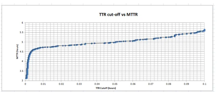
5.2 Behaviour of MTTR with respect to TTR Cut-off for the Site A Dataset ... 50

5.2.1 Critical Short TTR durations ... 50

5.2.2 Critical Long TTR durations ... 52

5.3 Filtering of Unscheduled Maintenance Down Time States with short durations for the Site A Dataset ... 53

5.3.1 Filtering of Short TTR Durations while Excluding Filtered Segments ... 53

5.3.2 Filtering of Short TTR Durations with addition of Filtered Segments back into preceding state ... 60

5.4 Filtering of Long Unscheduled Maintenance States durations for the Site A Dataset ... 65

5.4.1 Filtering of Long TTR Durations while Excluding Filtered Segments ... 65

5.4.2 Filtering of Long TTR Durations with addition of Filtered Segments back into Scheduled Maintenance Down Time Categories ... 70

5.5 Combined Filtering of Both Short and Long Unscheduled Maintenance State durations for the Site A Dataset (with addition of filtered segments back into the dataset)... 72

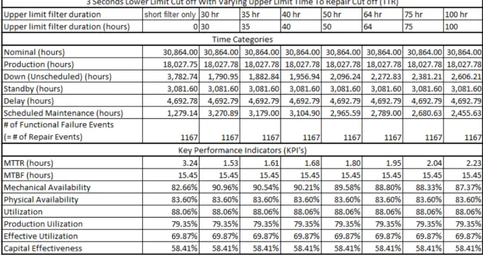
5.5.1 Maintaining the Short Duration Filter at 3 Seconds While Varying the Long Duration Filter .. 73

5.5.2 Maintaining the Short Duration Filter at 30 Minutes While Varying the Long Duration Filter 75 5.6 Behaviour of MTTR with respect to TTR Cut-off for the Site B Dataset ... 77

5.6.1 Critical Short TTR durations ... 77

5.6.2 Critical Long TTR durations ... 80

5.7 Filtering of short Unscheduled Maintenance State durations for Site B Dataset ... 80

5.7.1 Filtering of Short duration while excluding filtered segments from the Site B Dataset ... 80

5.7.2 Filtering of Short Durations with addition of filtered segments back in to the preceding State for Site B ... 84

5.8 Filtering of long Unscheduled Maintenance States durations for Site B Dataset ... 85

5.8.1 Filtering of Long TTR Durations while excluding the filtered segments from the dataset for Site B ... 85

5.8.2 Filtering of Long Repair durations with addition of filtered segments back in to total Scheduled Maintenance Down Time for Site B ... 89

5.9 Combined filtering of both Short and Long Unscheduled Maintenance State Durations for Site B Dataset ... 91

5.9.1 Maintaining the Short Duration Filter at 1.8 Minutes While Varying the Long Duration Filter91 5.9.2 Maintaining the Short Duration Filter at 9.6 Minutes While Varying the Long Duration Filter93 Chapter 6 Sensitivity of KPI’s to Filtering of Production States based on Duration of Time-Between-Failure (TBF) ... 96

6.1 Behaviour of MTBF with respect to TBF Cut-off for Site A Dataset... 97

6.2 Filtering of Production States with short durations for the Site A dataset ... 100

6.2.1 Filtering of Short TBF Durations for the Site A Dataset (while excluding filtered segments) 100 6.2.2 Filtering of short TBF Durations for Site A Dataset (with addition of filtered segments back into the dataset) ... 103

6.3 Behaviour of MTBF with respect to TBF Cut-off for Site A Dataset... 107

6.4 Filtering of Production States with short durations for the Site B dataset ... 110

6.4.1 Filtering of Short TBF Durations for Site B Dataset while Excluding Filtered Segments ... 110

6.4.2 Filtering of Short Time Between Failure Durations For Site B Dataset With Addition of Filtered Segments Back Into the Dataset ... 116

Chapter 7 Conclusions and Recommendations for Future Work ... 122

7.1 Conclusions ... 122

7.2 Primary Contributions ... 127

7.3 Recommendations for Future Work ... 127

References ... 129

List of Figures

Figure 1: Typical break down of open pit mining costs [Daneshmend, 2009] (courtesy of Modular

Mining). ... 2

Figure 2: Fleet management system data flow [Olson, 2011]. ... 7

Figure 3: Haul Truck MTBF at an open pit mine [Schouten, 1998]. ... 16

Figure 4: Average Down Time at the same open pit mine [Schouten, 1998]. ... 17

Figure 5: Model of algorithms used for dispatch optimization [Chapman, 2012]. ... 18

Figure 6 : Typical layout of the field computer display [Bonderoff, 2009]. ... 21

Figure 7 : Field computer input selection menu [Bonderoff, 2009]... 21

Figure 8 : Format of data gathered by a typical fleet management system [Modular Mining Systems, 2012]. ... 22

Figure 9 : Status records used for further analysis [Modular Mining Systems, 2012]. ... 23

Figure 10 “Maintenance Down” time category in the time model. ... 32

Figure 11 “Up Time” time category in the time model. ... 33

Figure 12. Typical time model. ... 36

Figure 13. Re-imagined time model. ... 36

Figure 14. How mechanical availability can be visualized in the time model. ... 38

Figure 15. How physical availability can be visualized in the time model. ... 41

Figure 16. How utilization can be visualized in the time model. ... 43

Figure 17. How production utilization can be visualized in the time model. ... 44

Figure 18. How effective utilization can be visualized in the time model. ... 46

Figure 19: Flow of analysis for investigation of TTR sensitivities. ... 49

Figure 20: Initial analysis plotting TTR durations versus MTTR (Site A dataset). ... 51

Figure 21: Initial analysis – zoomed on short TTR durations ... 52

Figure 22: Initial analysis – focused on long TTR durations. ... 53

Figure 23: Initial analysis – further zoomed on very short TTR durations. ... 54

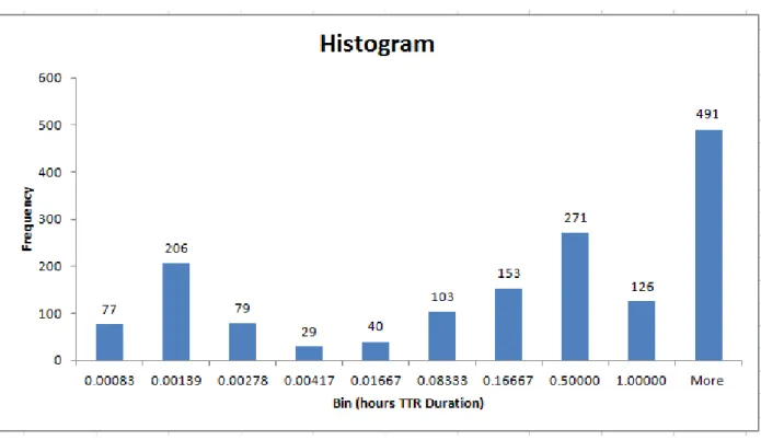
Figure 24: Histogram of Unscheduled Maintenance States, with bins corresponding to cut-off durations used in filtering analysis (Site A dataset) ... 55

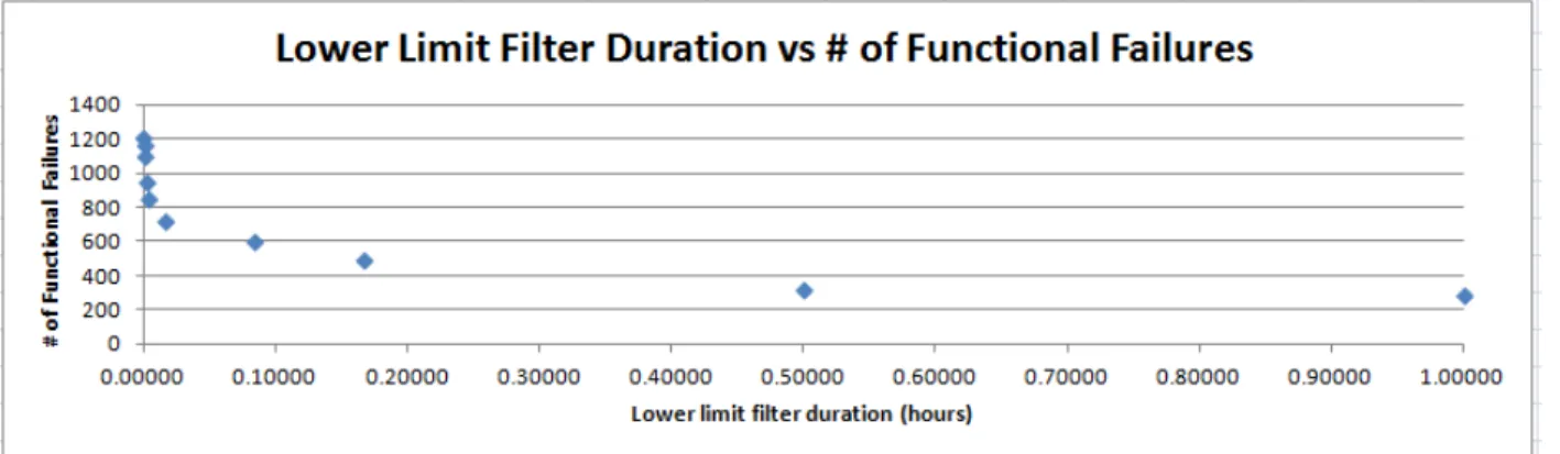
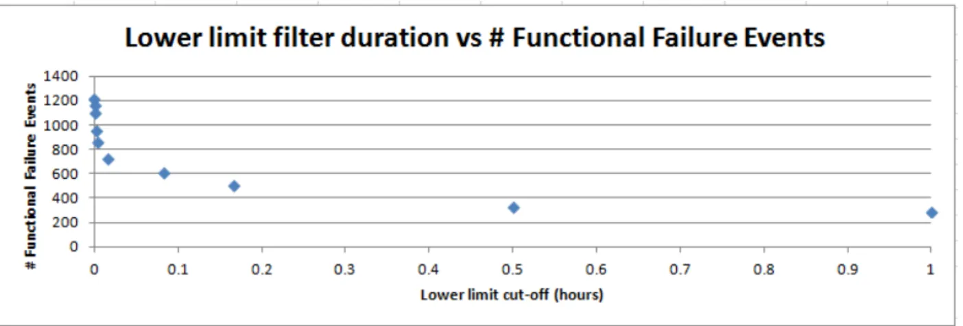
Figure 25: Number of functional failure events versus short TTR filter durations (while excluding filtered segments - Site A dataset). ... 57

Figure 26: MTTR versus TTR filter durations (while excluding filtered segments - Site A dataset). ... 57

Figure 27: MTBF versus TTR filter durations (while excluding filtered segments - Site A dataset) ... 58

Figure 28: Mechanical availability versus TTR filter durations (while excluding filtered segments - Site A dataset) ... 58 Figure 29: Physical availability versus TTR filter durations (while excluding filtered segments - Site A dataset). ... 59 Figure 30: Capital Effectiveness versus TTR filter durations (while excluding filtered segments - Site A dataset). ... 59 Figure 31: Number of functional failure events versus TTR filter durations (while adding filtered

segments to preceding state - Site A dataset). ... 61 Figure 32: Mean time to repair versus TTR filter durations (while adding filtered segments to preceding state - Site A dataset). ... 61 Figure 33: Mean time between failure versus TTR filter durations (while adding filtered segments to preceding state - Site A dataset). ... 62 Figure 34: Mechanical Availability versus TTR filter durations (while adding filtered segments to

preceding state - Site A dataset). ... 62 Figure 35: Physical availability versus TTR filter durations (while adding filtered segments to preceding state - Site A dataset). ... 63 Figure 36: Capital Effectiveness versus TTR filter durations (while adding filtered segments to preceding state - Site A dataset). ... 63 Figure 37 Utilization versus TTR filter durations (while adding filtered segments to preceding state - Site A dataset). ... 64 Figure 38: Production Utilization versus TTR filter durations (while adding filtered segments to preceding state - Site A dataset). ... 64 Figure 39 Effective Utilization versus TTR filter durations (while adding filtered segments to preceding state - Site A dataset). ... 65 Figure 40: Number of functional failure events versus long TTR filter durations (while excluding filtered segments - Site A dataset). ... 67 Figure 41: MTTR versus long TTR filter durations (while excluding filtered segments - Site A dataset). 67 Figure 42: MTBF versus long TTR filter durations (while excluding filtered segments - Site A dataset). 68 Figure 43: Mechanical Availability versus long TTR filter durations (while excluding filtered segments - Site A dataset). ... 68 Figure 44: Physical availability versus long TTR filter durations (while excluding filtered segments - Site A dataset). ... 69 Figure 45: Capital Effectiveness versus long TTR filter durations (while excluding filtered segments - Site A dataset). ... 69

Figure 46: MTTR versus long TTR filter durations (with addition of filtered segments back into total

scheduled maintenance down - Site A dataset). ... 71

Figure 47: Mechanical Availability versus long TTR filter durations (with addition of filtered segments back into total scheduled maintenance down - Site A dataset). ... 72

Figure 48: MTTR versus long TTR filter durations (with constant 3 second short duration filter and addition of filtered segments back into total scheduled maintenance down - Site A dataset). ... 74

Figure 49: Mechanical Availability versus long TTR filter durations (with constant 3 second short duration filter and addition of filtered segments back into total scheduled maintenance down - Site A dataset). ... 75

Figure 50: MTTR versus long TTR filter durations (with constant 30 minute short duration filter and addition of filtered segments back into total scheduled maintenance down - Site A dataset). ... 76

Figure 51: Mechanical availability versus Mean time to repair versus long TTR filter durations (with constant 30 minute short duration filter and addition of filtered segments back into total scheduled maintenance down - Site A dataset). ... 77

Figure 52: Initial analysis plotting TTR durations versus MTTR (Site B dataset). ... 78

Figure 53: Initial analysis plotting very short TTR durations versus MTTR. ... 78

Figure 54: Histogram of Unscheduled Maintenance States, with bins corresponding to cut-off durations used in filtering analysis (Site B dataset) ... 79

Figure 55: Initial analysis plotting TTR durations versus MTTR. ... 80

Figure 56: Number of functional failure events versus each TTR filter’s durations. ... 82

Figure 57: MTTR versus each TTR filter’s durations. ... 82

Figure 58: MTBF versus each TTR filter’s durations. ... 83

Figure 59: Mechanical availability using MTTR and MTBF versus each TTR filter’s durations. ... 83

Figure 60: Number of functional failure events versus long TTR filter durations (while excluding filtered segments - Site B dataset). ... 86

Figure 61: MTTR versus long TTR filter durations (while excluding filtered segments - Site B dataset). 86 Figure 62: MTBF versus long TTR filter durations (while excluding filtered segments - Site B dataset). 87 Figure 63: Mechanical Availability versus long TTR filter durations (while excluding filtered segments - Site B dataset) ... 87

Figure 64: Physical availability versus long TTR filter durations (while excluding filtered segments - Site B dataset). ... 88

Figure 65: Capital effectiveness versus long TTR filter durations (while excluding filtered segments - Site B dataset). ... 88

Figure 66: MTTR versus long TTR filter durations (with addition of filtered segments back into total

scheduled maintenance down – Site B dataset). ... 90

Figure 67: Mechanical Availability versus long TTR filter durations (with addition of filtered segments back into total scheduled maintenance down – Site B dataset). ... 90

Figure 68: MTTR versus long TTR filter durations (with constant 1.8 minutes short duration filter and addition of filtered segments back into total scheduled maintenance down – Site B dataset). ... 92

Figure 69: Mechanical Availability versus long TTR filter durations (with constant 1.8 minutes short duration filter and addition of filtered segments back into total scheduled maintenance down – Site B dataset). ... 93

Figure 70: MTTR versus long TTR filter durations (with constant 9.6 minute short duration filter and addition of filtered segments back into total scheduled maintenance down – Site B dataset). ... 94

Figure 71: Mechanical Availability versus long TTR filter durations (with constant 9.6 minute short duration filter and addition of filtered segments back into total scheduled maintenance down – Site B dataset). ... 95

Figure 72: Flow of analysis for investigation of TBF sensitivities. ... 96

Figure 73: Initial analysis plotting TBF durations versus MTBF (Site A dataset). ... 97

Figure 74: Initial analysis – further zoomed on very short TBF durations. ... 98

Figure 75: Histogram of Production States, with bins corresponding to cut-off durations used in filtering analysis (Site A dataset) ... 99

Figure 76: Number of functional failure events versus short TBF filter durations (while excluding filtered segments - Site A dataset). ... 101

Figure 77: MTTR versus short TBF filter durations (while excluding filtered segments - Site A dataset). ... 101

Figure 78: MTBF versus short TBF filter durations (while excluding filtered segments - Site A dataset). ... 102

Figure 79: Mechanical Availability versus short TBF filter durations (while excluding filtered segments - Site A dataset). ... 102

Figure 80: Number of functional failure events versus TBF filter durations (while adding filtered segments to preceding state - Site A dataset). ... 103

Figure 81: MTTR versus TBF filter durations (while adding filtered segments to preceding state - Site A dataset). ... 104

Figure 82: MTBF versus TBF filter durations (while adding filtered segments to preceding state - Site A dataset). ... 104

Figure 83: Mechanical Availability versus TBF filter durations (while adding filtered segments to

preceding state - Site A dataset). ... 105 Figure 84: Physical Availability versus TBF filter durations (while adding filtered segments to preceding state - Site A dataset). ... 105 Figure 85: Production Utilization versus TBF filter durations (while adding filtered segments to preceding state - Site A dataset). ... 106 Figure 86 Effective Utilization versus TBF filter durations (while adding filtered segments to preceding state - Site A dataset). ... 106 Figure 87: Capital Effectiveness versus TBF filter durations (while adding filtered segments to preceding state - Site A dataset). ... 107 Figure 88: Initial analysis plotting TBF durations versus MTBF. ... 107 Figure 89: Initial analysis – further zoomed on very short TBF durations. ... 108 Figure 90: Histogram of Production States, with bins corresponding to cut-off durations used in filtering analysis (Site B dataset) ... 109 Figure 91: Number of functional failure events versus short TBF filter durations (while excluding filtered segments - Site B dataset). ... 111 Figure 92: MTBF versus short TBF filter durations (while excluding filtered segments - Site B dataset). ... 111 Figure 93: MTTR versus short TBF filter durations (while excluding filtered segments - Site B dataset). ... 112 Figure 94: Mechanical Availability versus short TBF filter durations (while excluding filtered segments - Site B dataset). ... 112 Figure 95: Physical Availability versus short TBF filter durations (while excluding filtered segments - Site B dataset). ... 113 Figure 96: Utilization versus short TBF filter durations (while excluding filtered segments - Site B

dataset). ... 113 Figure 97: Production Utilization versus short TBF filter durations (while excluding filtered segments - Site B dataset). ... 114 Figure 98: Effective Utilization versus short TBF filter durations (while excluding filtered segments - Site B dataset). ... 114 Figure 99: Capital Effectiveness versus short TBF filter durations (while excluding filtered segments - Site B dataset). ... 115 Figure 100: Number of functional failure events versus TBF filter durations (while adding filtered

segments to preceding state - Site B dataset). ... 117 xii

Figure 101: MTTR versus TBF filter durations (while adding filtered segments to preceding state - Site B dataset). ... 117 Figure 102: MTBF versus TBF filter durations (while adding filtered segments to preceding state - Site B dataset). ... 118 Figure 103: Mechanical Availability versus TBF filter durations (while adding filtered segments to preceding state - Site B dataset). ... 118 Figure 104: Physical Availability versus TBF filter durations (while adding filtered segments to preceding state - Site B dataset). ... 119 Figure 105: Utilization versus TBF filter durations (while adding filtered segments to preceding state - Site B dataset). ... 119 Figure 106: Production Utilization versus TBF filter durations (while adding filtered segments to

preceding state - Site B dataset). ... 120 Figure 107: Effective Utilization versus TBF filter durations (while adding filtered segments to preceding state - Site B dataset). ... 120 Figure 108: Capital Effectiveness versus TBF filter durations (while adding filtered segments to

preceding state - Site B dataset). ... 121

List of Tables

Table 1. Reference MTBF, MTTR, and availability [Lewis, 2007]. ... 15 Table 2. Transition frequencies of the Site B dataset... 35 Table 3: Distribution of Unscheduled Maintenance States, with bins corresponding to cut-off durations used in filtering analysis (Site A dataset) ... 54 Table 4: Filtering of Unscheduled Maintenance States with short durations while excluding filtered segments for Site A dataset. ... 56 Table 5: Filtering of short Unscheduled Maintenance State durations with addition of filtered segments back in to the preceding state for Site A dataset. ... 60 Table 6: Filtering of long Unscheduled Maintenance States durations while excluding filtered segments from the dataset for Site A. ... 66 Table 7: Filtering of long Unscheduled Maintenance State durations with addition of filtered segments back into total scheduled maintenance down time for Site A ... 71 Table 8: Maintaining the short duration filter at 3 seconds while varying the long duration filter. ... 74 Table 9: Maintaining the short duration filter at 30 minutes while varying the long duration filter. ... 76 Table 10: Distribution of Unscheduled Maintenance States, with bins corresponding to cut-off durations used in filtering analysis (Site B dataset) ... 79 Table 11: Filtering of short duration while excluding filtered segments from the Site B dataset. ... 81 Table 12: Filtering of short durations with addition of filtered segments back in to the preceding state for Site B ... 84 Table 13: Filtering of Long Repair Durations While Excluding the Filtered Segments from the Dataset for Site B. ... 85 Table 14: Filtering of long repair durations with addition of filtered segments back in to total scheduled maintenance down time for Site B ... 89 Table 15: Maintaining the short duration filter at 1.8 minutes while varying the long duration filter... 92 Table 16: Maintaining the short duration filter at 9.6 minutes while varying the long duration filter... 94 Table 17: Distribution of Production States, with bins corresponding to cut-off durations used in filtering analysis (Site A dataset) ... 99 Table 18: Filtering of short TBF durations while excluding filtered segments for Site A dataset. ... 100 Table 19: Filtering of short TBF durations with addition of filtered segments back in to the preceding state for Site A dataset. ... 103 Table 20: Distribution of Production States, with bins corresponding to cut-off durations used in filtering analysis (Site B dataset) ... 108

Table 21: Filtering of short TBF durations while excluding filtered segments for Site B dataset. ... 110 Table 22: Filtering of short TBF durations with addition of filtered segments back in to the preceding state for Site B dataset. ... 116

Chapter 1

Introduction

1.1 Raw Data and Analysis of Data Quality

Like many industries centered around cyclical processes, the open pit mining sector seeks to maximize the bottom line through process optimization. Given that the net earnings (bottom-line) is dictated by countless factors, it is practical for a mine site to focus on controllable aspects within its operation: for example reducing operating costs and increasing throughput of materials handled. Analysis of historical data on equipment activity that is collected by a mine site's Fleet Management System (FMS) is

fundamental for production planning, as well as maintenance planning – optimization of both of which is essential for competing in today's mining industry.

Large open pit mines utilize fleets of haul trucks to transport ore and waste from the pit; but in order to manage and track the allocation of these complex and costly machines, the majority of today's open pit mines employ some form of FMS – which consists of both software and hardware components. In general, analysis on sequential data queried from historical databases (collected by the FMS) is the primary means of measuring and assessing the reliability, maintenance effectiveness, and production efficiency of mining haul trucks. These measures and assessments are then factored into operations and production planning. For example, the dispatch coordination team can increase the overall production time through decreasing man hours lost to logistical inefficiencies through better planning or improving equipment life through quantitatively measuring maintenance performance; these practices ultimately improve the bottom line.

In addition, further analysis on FMS data streams can also provide the foundation for maintenance planning and investigating causes of failure. Using these data streams, Key Performance Indicators (KPI’s) can be calculated to provide quantifiable metrics used as a quick reference by mine managers as to the effectiveness of operations management, production management, the effectiveness of maintenance

policies and most importantly, where to focus improvement efforts. As shown in the diagram below, maintenance related costs typically account for approximately 41% of total costs for open pit mines.

Figure 1: Typical break down of open pit mining costs [Daneshmend, 2009] (courtesy of Modular Mining).

The most fundamental reliability and maintenance metrics used for gauging haul truck fleet performance are Mean Time Between Failure (MTBF), and Mean Time To Repair (MTTR). Furthermore, with increasing interest in automation by the mining industry, these data streams generated by FMS’s are becoming ever more important due to the use of predictive simulations.

KPI is a general term encompassing performance metrics used by many organizations for measuring the success of a specified activity. In general, industries such as the mining sector will use similar KPIs to evaluate common operating activities. Due to the cyclical nature of open pit mining truck haulage activities, continual improvements in the management of mining equipment will require the use of time-based quantitative KPI's

1.2 Problem Definition and Thesis Objectives

The primary objective of this thesis is to examine the raw data acquired from an FMS, and determine if any data quality issues can be identified. Based on the identified quality issues, the next objective is to determine whether some form of processing or filtering of the raw data can improve the FMS data quality. Finally, the thesis aims to investigate what the impacts of FMS data quality might be on selected KPI’s.

This thesis focuses on the impacts of FMS data quality on the following KPI’s:

• Mean Time Between Failure (MTBF)

• Mean Time To Repair (MTTR)

• Availability: both Mechanical Availability and Physical Availability

• Utilization, Production Utilization, and Effective Utilization

• Capital Effectiveness

These are chosen because they are most frequently used for operations planning and maintenance planning in order to improve efficiency at mines.

1.3 Methodology

This thesis builds upon Barrick's time model [Barrick, 2006] which includes definitions for the KPI's of interest (except for Mechanical Availability), and event classification / categorization schemes.

The datasets collected from two different FMS’s, at two distinct mine sites are investigated (i.e. each dataset is obtained from a different FMS vendor, at a different mine site).

The first dataset is from an open pit gold mine located in the Site A mining district of central-east Chile – the Site A mine. This dataset was collected on 16 CAT 785 haul trucks and represents roughly 30,000 hours of operation (3 months of operation from October to the end of December in the year 2009). The second dataset was also from an open pit gold mine: the Site B mine, located in the Atacama Region of

northern Chile. This second dataset was for a fleet of 13 CAT 785 haul trucks, and represents roughly 10,000 hours of operation (one month of data, in the last month of 2009).

Analysis of the raw datasets focuses on durations of states, and whether state durations are “valid” – on the basis of either being too short to be feasible, or too long to have been correctly categorized.

1.4 Thesis Overview

Chapter 2 consists of a literature review, covering fleet management systems, data quality and

management philosophies with focus on the application of six sigma philosophy on data analysis, as well as relevant KPIs, as well as haul truck automation. In Chapter 3 the data collection, classification, and representation process typically used by an FMS is discussed. A detailed review of how KPI's are calculated from a specific, commonly used, time model is provided in Chapter 4.

In Chapter 5, sensitivity analyses on KPI’s to the effects of applying filters on Unscheduled Maintenance Down Time states in the dataset are examined; these filters are based on Time To Repair (TTR) durations. Chapter 6 replicates the same analyses as in Chapter 5, but instead applies filters on Production states based on Time To Failure (TTF) durations

Conclusions, primary contributions, and recommendations for future work are presented in Chapter 7.

Chapter 2

Literature Review

2.1 History of Data Collection

In 1979, when wireless data transfer was in the early stages of development, the highest rate of data transfer was only 1200 bits per second. Today, after more than thirty years of technological advancement, fleet management systems have the capability to transfer data exceeding rates of 10 megabits per second, approximately 10,000 times the rate compared to its beginning [Zoschke, 2001]. In addition, both data collection hardware and software have improved in the quantity of input parameters to provide more accurate simulations of mine operations. In turn, this allows for better management in all aspects of the equipment quantitatively rather than trial and error. Compared to having a foreman manually directing pieces of equipment to areas he feels is fit, current fleet management systems have the capability to monitor important aspects of a mine site in real time and utilize mathematical algorithms to optimizing equipment allocation. In addition, improvements in data storage capacities now allows for a greater range of mine site activities to be recorded into historical databases. Due to the large quantity of data collected on a day to day basis specified queries can also be performed by the dispatch software to extract specific portions from within the collected raw datasets. For the purpose of examining haul truck KPI's, a query on the raw database can be performed to extract data only concerning haul trucks, in sequential form, for further calculations.

2.2 Dispatch system providers

Currently Modular Mining Systems, Wenco International Mining Systems Limited, and Leica Geosystems are the leading providers for fleet management hardware and software. Modular Mining Systems offers the DISPATCH system which is customizable for both open pit and underground mines [Modular Mining Systems, 2012]. Leica Geosystems offer a package called Leica Jigsaw Fleet

Management System (Jfleet) [Leica Geosystems, 2014]. And Wenco International Mining Systems Limited offers Wencomine fleet management system [Wenco International Mining Systems Limited,

2014]. Although each company offers unique solutions to managing equipment fleets, they all essentially provide the capability to track and monitor equipment location, production, maintenance, and safety through GPS and wireless radio networks. This chapter will focus primarily focus on Modular Mining System’s approach in collecting haul truck data.

2.3 Overview and History of Modular Dispatch

Modular Mining Systems Inc.'s DispatchTM _{is a fleet managing system containing a wide range of} capabilities for managing a fleet of equipment such as in an open pit mine. The system contains multiple databases: the haulage model database portion of the software generates real-time models of an equipment fleet with the option for the user to manually modify the operating parameters while operations are live. Secondarily the software's reporting database records historical data on a shift by shift basis. From this historical database users can choose to display specified portions of the raw data for further analysis, such as in this thesis. In conjunction with each stored database are customizable directories in the form of enumerated tables which are built into the software for more efficient data storage. Databases used for the haulage model, reporting database, and enumerated tables are key elements within an FMS for collecting and quantifying daily equipment activities. Included with the software are operating manuals which were used as a starting point for understanding how truck fleet state transitions are generally recorded by a mine operation’s fleet management system. The diagram below shows a simplified representation of data flow.

Figure 2: Fleet management system data flow [Olson, 2011].

2.4 Current Practice of Utilizing Data for KPI

Although numerous investigations have been focused on understanding the topic of using KPIs for improving production planning, sensitivity analysis of large datasets, and fleet management systems, little or no work has been done on performing data quality analysis on sequential data collected by a fleet management system for the purpose of calculating KPIs. Given that this paper focuses on the quality of these sequential datasets, it is appropriate to tie the different areas of research together to gain a picture of the current understanding with regards to the analysis implemented in this thesis.

KPI’s are the basis for measuring performance for most businesses, thus they are essential in all aspects of planning for cyclical processes. When planning any complex process, different KPIs will have increasing levels of uncertainty [Marz, 2012] as the scope and how far into the future the plan is from the present increases: i.e. short term planning will be much more accurate than long term planning. It is important to recognize that although each level of planning serves different levels of decision making in an

organization, they all have mutual influence because they are based on an established set of KPIs. As indicated cycle times are often the limiting factor for assembly line type processes, which is similar to haul truck production cycles [Marz, 2012]. In other industries, it is common to use computers to simulate

cyclical processes through the use of KPIs. Since production planning is mainly based on KPIs derived from historical databases, it is of the utmost importance that these KPI’s are precise and accurate in order to generate effective plans and maximize productive hours of work [Modular Mining Systems, 2012]. A lot of research in the field of optimizing truck and shovel assignments has been done; much of the optimization process require expertise in order to factor in real life constraints [Ercelebi and Bascetin, 2009]. These constraints can be identified by historical databases, to be more specific, raw sequential data. Using models built upon identified constraints that are determined by historical databases, truck routes and allocations can then be simulated [Subtil, et al., 2011]. This is why fleet management systems have become so important in the process of planning, selecting fleet sizes and optimization of truck routes. Before the mid 1970’s trucks were assigned on a trip by trip basis and also by the intuition of a dispatcher; this resulted in inefficient processes when compared to today’s standards and ability to process large amounts of data though computers [Richards, 2000]. Even right up to the present day, it is standard practice for some mines to allocate a set of trucks to each operating loader at the start of a shift based on the production requirements for the day. It is clear that, due to the changing terrain for mining operations, this fixed allocation technique has many shortcomings compared to a system which reassigns each truck on a trip by trip basis and recalculates the base of changing states [Scheaffer and McClave, 1995].

Through the advent of fleet management systems along with the use of optimization algorithms, proper planning and reporting, the shortcomings of reactive decisions can be overcome [Dantzig and Ramser, 1959]. This type of research and application extends to other dispatching services such as delivery, courier and emergency response [Culley, et al., 1994].

Furthermore after the mid 1990’s the indoctrination of “context-aware maintenance support system” has become an integral part at all levels of planning in order to complete with the ever increasing competitive nature of industries such as mining. Metrics such as KPI’s allows a team to make decisions associated

with improving production planning such as the ratio of trucks to shovels [Kolonja and Mutmansky, 1993].

Due to the variability that exists from operation to operation, a broad range of different KPI’s are used to measure similar processes. However, a new problem has been identified: the subjective nature of how performance is measured; this leads to issues with inconsistency and inability to benchmark within the mining industry. In addition, due to the rapid turnover rate of employment in the mining industry, the inability to retain skill and expertise is also becoming a problem [Mathew, et al., 2011]. To elaborate, organizational boundaries in terms of expertise have broadened to resemble service networks; highly specialized understanding of complex processes are typically contracted out to avoid risk. Although this strategy is adaptive in today’s competitive market for the short term, the opportunity for knowledge retention and a deep understanding of each operation’s processes is lost. This leads to the issue of truly understanding and interpreting each company’s localized KPIs. It is widely mistaken that a short-term fix of this problem is resolved through the use of customized simulation models, data collection, calibration and validation software and hardware. Although customized simulation models are providing quantitative advice in terms of allocating resources, the opportunity to further optimize processes within the operation requires years of accumulated knowledge in order to be realized [Tywoniak, et al. 2008].

Among the academic community, it has also been recognized that an issue exists on the subject of data quality. Poor data quality leads to lost productivity, higher error rates for planning and the inability to accurately make high impact decisions. In addition, attempts to predict asset reliability and long term performance will be completely misguided by erroneous data. Many attempts have been made to define what data quality means. In general, it is understood that accuracy, relevance, fineness and timeliness are some of the requirements. This issue within the mining sector is one that most well established companies are aware of but avoid due to the expensive and time-consuming effort required. Regardless of how good the data collection mechanism is, if there is not enough expertise to calibrate the data collection process to meet the needs of further analysis, the investment is not able to generate optimal results. It is necessary to

invest in understanding the dynamics of overall equipment effectiveness as part of a system to enhance asset management practices [Zuashkiani, et al., 2011]. Strong evidence suggests that most organizations possess much more data than they need or actually utilize for further analysis. Above all, the surplus of data can make the portion of the dataset required for analysis harder to extract. As well, the lack of data visibility and interpretation reduces the accuracy and precision in the dataset. These factors ultimately lead to less effective planning decisions, and the inability to improve the process of concern [Lin, et al., 2006]. For the above reasons, this thesis focuses on the issue of data quality.

2.5 Six Sigma and Data Quality

In light of the desire to improve the bottom line through effective equipment management, as with other well established industries, much of the mining sector has adopted an overarching philosophy of

continuous improvement processes centered on optimizing operational efficiency, effectiveness and flexibility of manageable aspects within the workplace. Consistent with that philosophy, this thesis is focused on a subset of the continuous improvement process known as Six Sigma. This section begins by addressing the first step of the DMAIC process (define, measure, analyze, improve and control) which is defining the end goal of improving KPIs performance used for measuring truck haulage performance. Only through establishing a precise definition of these performance metrics, can an accurate interpretation of the available datasets be achieved. Next, this paper addresses the second and third steps of the DMAIC process by investigating the data quality of the datasets used in calculating these key performance

indicator metrics.

Like many continuous improvement theories, Six Sigma is also a philosophy for improving a process through continually reducing costs which ultimately translates to increased profits. Although Six Sigma is typically implemented on repetitive and well established processes, this method of continual improvement can also be applied to the management of open pit mining haulage operations. Specifically, the process of transporting the ore from the mining face to the dump location presents opportunities for implementing the Six Sigma philosophy thus improving truck fleet performance. Initially, Six Sigma methodologies were employed to reduce the average number of defects in the manufacturing industry; however, the less

well-known aspect of Six Sigma seeks to reduce deviations from specified levels of performance. This aspect of continuous improvement makes Six Sigma a very applicable method for reducing costs for the mining industry due to the cyclical nature of many of its processes and its tendency to deviate from optimal performance. As this paper is focused on improving the efficiency and effectiveness of data collected pertaining to truck haulage by fleet management systems, a continuous improvement process such as Six Sigma can be applied to help ensure data collected is indeed essential, and as well, further data analysis performed on the data collected is accurate, precise and necessary to improve the process of KPI analysis. Data quality is the key to accurate KPI calculations, which are essentially the representation of mine operations performance used for production planning.

To begin the integration of the Six Sigma philosophy into a process, it is helpful to utilize the

abbreviation DMAIC. This abbreviation, as previously mentioned, is a roadmap defining the steps from beginning to end for achieving improvements in a process. DMAIC stands for Define, Measure, Analyze, Improve and Control [Desai and Shrivastava, 2008]. Although many continuous improvement processes inherently seeks to attain the same goal of improving the efficiency and effectiveness of a process, DMAIC provides a methodical framework for identifying which areas of a process requires attention. The DMAIC process will be applied in this section to the haul truck fleet management's data collection process to show how data quality can be improved and how it affects the resulting KPI calculations. Although it is well established that mining trucks constantly face changing environments, the required tasks for transporting ore generally remains a cyclical task. This cyclical nature allows the

implementation of data collection regimes for the purpose of documentation, but more importantly the evaluation of a mine's performance. Because this collected data is measuring a very complex process, often the dataset collected includes too much information; some of which can be inaccurately included in KPI calculations, this mistake will often lead to an inaccurate representation of the process' performance. The means to accomplishing the six sigma goals is to identify the processes where no value is added, and to eliminate steps in the process where unnecessary rework exists [Hassan, 2013].

2.5.1 Define

The first step of the DMAIC is defining the scope, goal or objective of an improvement process. This initial step sets the boundaries of a process and allows focus to be directed on the identified problems through limiting the amount of variables. After setting boundaries, components within the process can then be separated as either controllable or uncontrollable. In accordance with the "Defining" step of the DMAIC process, the goal of improving the data quality of data collected by a fleet management system and the data analysis process, the boundaries must first be defined [Cordy and Coryea, 2006]. The scope of this paper specifically looks at data collected on haul trucks through a fleet management system with the end goal of generating a more accurate representation of haul truck performance pertaining to maintenance and allocation of resources.

Fundamentally, the sole purpose of this data collection process is to allow management to perform mine planning and quantitatively assess how operations are performing. This then allows management to identify which areas of the mining operation can be targeted for improvement. Thus, it is important that this step of the "Defining" process accurately represents what is happening in the data collection process. Just as important is that this step accurately defines the process of calculating KPI's to ensure the

calculations are performed using relevant portions of the dataset and the resulting metrics are not skewed due to misinterpretations of the raw data. In accordance with the Six Sigma philosophy, every step within the process outlined above should have value added, whereby each step is necessary for the defined goal; each step has an impact on the process and each step is done right the first time. By ensuring these three guidelines, the Six Sigma philosophy will provide more efficient use of resources such as capital, labor and time. Essentially, the defined process of data collection is effectively meeting the needs and requirements of the objective, which is to quantify the level of performance of a haulage process.

2.5.2 Measure

As previously mentioned, in order to gauge the performance of each individual haul truck or the entire fleet, the process begins with an operator's input of what is happening in the field. This information is

collected in the form of raw data through a fleet management system, from which the sequential data can then be extracted. The dataset used for further analysis encompasses the documentation of every event change, the durations of each event, and a time stamp of each truck in the fleet. Secondarily, a time model unique to each mine is used as a guide for categorizing each event in to its corresponding time category. Once the time categories for each documented event have been added on to the dataset, further analysis such as KPI calculations can be performed.

As mentioned, to quantify the performance of a haul truck fleet, key performance indicators are used. These KPI’s typically include MTTR, MTBF, Mechanical Availability, Physical Availability, Utilization, Production Utilization, Effective Utilization, and Capital Effectiveness. These performance indicators essentially examine the total duration that the truck fleet spends in each time category in the form of ratios made up of conglomerates of each time category in order to reveal the performance of controllable

aspects associated with the truck fleet's performance. The key to this step in the DMAIC process is to compare truck fleet performance from period to period; this reveals unacceptable deviations from a specified level of performance. In essence, these KPI's reflect how efficient and effective the defined process is.

2.5.3 Analyze

The “Analyze” step in the DMAIC process is where expertise and experience in a defined process can help generate the most improvements. Of this entire data collection and analysis process for fleet management, it is important to identify controllable or manageable factors which are:

Operator and software interface

How accurately and precisely the operator is inputting what is actually happening with the haul truck during its defined nominal time.

Software and hardware

How much detail is documented by the data collection process and the accuracy and precision of data collected.

Raw dataset

Analyze the accuracy and precision of the data and, just as importantly, the suitability of the data collected which is to be used for key performance indicator calculations.

These controllable factors are areas of intervention where management can significantly improve the accuracy of the resulting measurements of haul truck performance. Furthermore, this improvement in the accuracy of performance metrics allows supervision to better identify areas within the production side of operations to target for improvements.

2.5.4 Improve

The “Improve” phase requires profound knowledge with respect to the process and is the step where improvements are conceptualized and tested. For the fleet management data collection and analysis process previously defined, the “Improve” phase seeks to remove erroneous, irrelevant or unnecessary data. In order to identify which data points are relevant to the later steps, sensitivity analysis can be employed to improve overall data quality. After identifying which data points are not required for the purpose of calculating key performance indicators accurately, the data collection process can be improved again by using filters on the sequential dataset or even better, modifying the fleet management software or hardware. Secondarily, because erroneous data is also caused by operator input, better training can ensure precise and accurate operator input, thus reducing inaccuracy for KPI calculations later in the process chain. In applying these improvements, fewer data points will be collected which results in less costs for the process, less cost for data storage, less time spent for data analysis, increased accuracy in key performance indicators and ultimately more effective mine planning.

2.5.5 Control

The “Control” step is the last step in the Six Sigma DMAIC process and is often the most difficult to maintain. Once improvements have been realized from the previous steps, the control phase seeks to maintain the new level of performance. The main objective is to ensure previous defects do not reoccur, and the improvements in the process become the new standard. The reason this phase is the most difficult

to achieve for any mine site is because of the high turnover rates in expertise in the mining industry. Often the experience and expertise initially required to implement and maintain the new found improvements are lost due the inadequacy by the mining industry in capturing the new found knowledge.

2.6 Other Literature Review

2.6.1 Comparative Values for MTBF, MTTR, and Mechanical Availability

Table 1. Reference MTBF, MTTR, and availability [Lewis, 2007].

The data above are values of MTBF, MTTR and Availability for 16 old Caterpillar 793s, 30 new

Komatsu 930Es, and 10 new and 14 old Caterpillar 797s at Suncor Energy Inc. oil sands operation in the Athabasca region of Northern Alberta. One year's worth of data which consisted of roughly 637,000 lines of data was used to calculate the KPI's above, these values act as a guideline as to typical MTBF, MTTR, and availability values. Taking the average of all the haul trucks and converting the values to hours, the entire fleet has a MTBF of 20.1 hours, MTTR of 2.7 hours, and Mechanical Availability of 87.75%.

Figure 3: Haul Truck MTBF at an open pit mine [Schouten, 1998].

In comparison, Figure 3 shows the distribution of MTBF of a large open pit mine in North America with seventy 190 ton Komatsu 685E haul trucks, and represents 2 years of operating data. Within two standard deviations above and below the mean, the MTBF is in the range of 17 to 31 hours. A value of 23 is used as the MTBF.

Figure 4: Average Down Time at the same open pit mine [Schouten, 1998].

In addition, for this same 70-truck fleet of 685E’s, using the data collected on Down Time over the first eight months of operation in 1997, the MTTR is approximately 2 hours. Then using these MTTR and MTBF values, the mechanical availability is calculated to be 92%.

2.6.2 Autonomous Haul Trucks

On a related note, recently there has been a big push towards automating mining equipment due to a shortage of haul truck operators and increased labor costs in some countries, notably Australia [Bellamy, 2011]. In light of this opportunity, major haul truck manufacturers have developed technologies to fully automate haul trucks to potentially increase availability and utilization through more consistent driving [Zoschke, 2001]. However, assuming automated driving does provide benefits in the aforementioned KPIs, one potential disadvantage to be considered is the loss of "front line maintenance"; typically the operator provides valuable information in to the failure modes through observation of irregularities in the equipment’s operation. This absence of the observer can potentially result in longer MTTR due to the extended time it takes to diagnose the failure mode and find the solution for repair.

Furthermore, in order to achieve fully automate mining equipment such as haul trucks, additional systems would need to be installed. This then increases the complexity of the haul trucks which potentially results in additional failure modes. In short, more failure modes can lead to a lower MTBF unless the consistency

of driverless technology significantly outweighs the resulting failure rates added from autonomous system components.

Many studies have been conducted to assess the economic benefits of autonomous haul truck operation. This effort is grounded on the assumption that reliability and maintainability metrics are accurate and a good representation of the wide range of operating conditions from mine to mine. This assumption however, may be false. Furthermore, the studies disregard the potential increase in MTTR and decrease in MTBF due to reasons previously mentioned.

2.6.3 Dispatch Algorithms

Figure 5: Model of algorithms used for dispatch optimization [Chapman, 2012]. In the structure of algorithms used for optimizing fleet dispatch, it can be seen that equipment breakdowns is a parameter that triggers re-computation of the model [White, et al., 1982].

It is important to re-evaluate what the purpose and use of the data in order to properly define the parameters of the algorithm. Similar to the idea of the computation model it is also important to specify the purpose of the dataset in order to further process the data. More specifically, cut-off ranges for data must be defined in order to perform accurate KPI calculations.

Using this form of algorithm model for optimizing haul fleets, which is essentially a model that tries to meet the highest possible predetermined KPI's by varying parameters such as dump locations, the importance of separating parameter definition from data gathering and data processing (what is used for KPI calculations) can be realized [Carter, 2010]. As explained in this chapter, the process of collecting data contains innumerable steps where errors by the software or hardware and mistakes by the operator can occur.

Chapter 3

Data Collection and Interpretation

3.1 Data Collection Process Overview

The quality of raw data often poses an issue in the precision and accuracy of results from further analysis. Multiple causes can account for deviation in data measurements from actual behavior in the field. First, because mining operations exist all around the world, and data is collected in different languages, information can be altered or lost during the translation process. In addition, due to the unique nature of every mine's management approach and the subjective nature of the collection process, inconsistencies exists in the definitions of mining terminology, categorization of events, structure of time models and other minor details from mine to mine. This lack of precision within the mining industry makes

benchmarking of operations performance problematic. Additionally, causes for poor quality of raw data collected can also be influenced by each operator's interpretation of input parameters. It is rare that every equipment operator has an accuracy of one hundred percent in his or her reporting practice. And

secondary causes can also be attributed to the effectiveness of the dispatch offices oversight. Both the quality in which status changes are documented, as well as data on failure causes has significant implications for further analysis.

As mentioned, an equipment operator plays an important role in the performance of the equipment. Specifically for haul trucks on a mine site, each operator may drive the hauls trucks in a different manner. In short, the operator’s operating practices have massive implications on the reliability of the truck and just as important, the equipment status reporting process.

Figure 6 : Typical layout of the field computer display [Bonderoff, 2009].

The field computer system is the interface that operators interact with. Generally, operators will input status and status changes by selecting the input from a range of options. Simultaneously, a time stamp will be entered each time the status has been changed. In addition, more information is usually provided such as the classification of the status, the reason code for the status change, and comments. The diagram below shows the typical arrangement of the field computer monitor.

Figure 7 : Field computer input selection menu [Bonderoff, 2009].

The central computer is where the information collected on haul truck activity is stored. From the central computer, dispatch managers can monitor a truck’s weight, tire condition, drive system, engine, and location. The FMS monitors and records every piece of mining equipment status and event in real time.

This data stream comprises equipment ID, when the equipment changed status, what the new status is, the reason code and reason for the status change, additional dispatcher comments and the length of time in each time category. The dispatching office provides oversight for day to day equipment operations. A truck's location and movement can be seen on the dispatch offices computer monitor, whereby if a piece of equipment is operating irregularly, the dispatcher will radio in and investigate the reason for the deviation. A database is also created and stored in a central computer in chronological order. In addition, this database can be manually entered or edited.

Figure 8 : Format of data gathered by a typical fleet management system [Modular Mining Systems, 2012].

Specified portions of data can be displayed or extracted by querying for a specific time frame, and for specific pieces of equipment or fleets of equipment can be selected from the raw database.

From the raw dataset, the status records can be extracted in the form of sequential data for further analysis.

Figure 9 : Status records used for further analysis [Modular Mining Systems, 2012].

It is imperative that every possible equipment status in the mine site is clearly defined in order to maintain consistency. By having a standardized time model, a mining company is able to reduce variability from the start of the data analysis process. The Barrick Time Model [Barrick, 2006] provides the basis for analysis of FMS data in this thesis. As will be defined in section 3.3, each status must be interpreted correctly in order to accurately calculate KPIs. Secondarily, because each documented status falls within a time category classification, the time categories must be precisely defined in order to maintain

consistency later in the analysis process.

3.2 Database for Reporting and Database for Haulage Model

Typically a tool is provided in a FMS for displaying, finding, creating, changing, and deleting data collected in the database. Within this database, records on normal operations are stored on a shift by shift basis. The records are segmented into load records, dump records, status records, fuel records, tram records, grade records, equipment records, auxiliary equipment records, location records, operator records and root information records. This tool also allows the user to output raw data in a specified summarized form. Shown in Figure 8 is the format in which the different datasets are collected.

3.2.2 Database for Haulage Model

The Database used for modeling haulage allocation is used for management of equipment fleets when operations are live. This dynamic model within a FMS is the basis on which algorithms for optimizing equipment task assignment operate. Stored within this database are the coordinates of all active locations, the orientation and availability of haulage roads, travel distances, travel times between haulage routes, real time haul truck status, mining constraints and operator information. Production data constantly flows

from the field to update the central database. This working model of haul truck activity allows the dispatcher to monitor and manage operations from the dispatch office.

3.2.3 Status, Reason, and Comment Field

The Status Records within the Reporting Database displays the time of each status change (Ready, Delay, Available, or Down), a reason code (what the reason was), comments, hours spent in each time category (operating hours, delay hours, availability/no operator hours (standby), or repairs/down hours). The table in Figure 9 shows the typical format in which this data is recorded.

Truck states are defined as either Ready, Delay, Available, or Down. Each data point under the “Hours in Time Category” is the duration of each status since the time stamp (under the “Time” column) of each status began. To elaborate, a status of “Delay” is the initial time stamp for when Operator Delay hours begins.

3.2.4 Reason

The Reason column records preprogrammed options selected by the equipment operator from the Field Computer System. Each Reason is mapped to a Code (integer) in an enumerated table. Using this method of data storage allows for improved efficiency in the volume of data stored. This column of the Status Records provides details on why each transition occurred for planning and maintenance purposes.

3.2.5 Comments

The Comment column of the Status Records collects information which is manually inputted by the operator. This data provides details on state transitions that deviate from normal mine operation. The information collected in this section can help in failure mode identification. For example, the comment section can provide the operator’s input concerning the context of a failure event.

3.3 Event Time Categories

Time categories can vary from mine site to mine site. In order to improve the accuracy of industry equipment performance benchmarking, it is logical to make the time categories used in the KPI's

standardized as well. Currently, the definition of time categories and classifications of events into time categories remain inconsistent in the industry. As well, terminology can be inconsistent due to language and translation discrepancies. An example is differences in time models between Site B and Site A. Major differences include time categories where Site A has unscheduled delay time and programmed delay time, whereas Site B only has delay time. In addition, due to the subjective nature of interpreting which time category each event falls into, there are many differences in the classification of events in to similar time categories; most notably Operating Delay and Operating Standby. For example, where Site A classifies shift change time as programmed delays (Delay time); Site B classifies shift change time into operating standby.

3.3.2 Nominal Time

Nominal time is the period of time that is being evaluated. This period of time in a mining operation is the sum of every possible time category. Nominal time is the sum of operating delay time, operating standby time, scheduled maintenance time, unscheduled maintenance time, primary production time and

secondary production time. 3.3.3 Delay Time

As defined by Barrick, operating delay time is, "Delays during an operating shift that are not necessarily related to a typical production cycle." To elaborate delay time represents the durations for haul trucks to get into production and is largely influenced by operator and effectiveness in truck allocation.

𝐷𝐷𝐷𝐷𝐷𝐷𝐷𝐷𝐷𝐷 𝑇𝑇𝑇𝑇𝑇𝑇𝐷𝐷=𝑁𝑁𝑁𝑁𝑇𝑇𝑇𝑇𝑁𝑁𝐷𝐷𝐷𝐷 𝑇𝑇𝑇𝑇𝑇𝑇𝐷𝐷 − 𝑃𝑃𝑃𝑃𝑁𝑁𝑃𝑃𝑃𝑃𝑃𝑃𝑃𝑃𝑇𝑇𝑁𝑁𝑁𝑁 𝑇𝑇𝑇𝑇𝑇𝑇𝐷𝐷 − 𝑆𝑆𝑃𝑃𝐷𝐷𝑁𝑁𝑃𝑃𝑆𝑆𝐷𝐷 𝑇𝑇𝑇𝑇𝑇𝑇𝐷𝐷 − 𝑆𝑆𝑃𝑃ℎ𝐷𝐷𝑃𝑃𝑃𝑃𝐷𝐷𝐷𝐷𝑃𝑃 𝑀𝑀𝐷𝐷𝑇𝑇𝑁𝑁𝑃𝑃𝐷𝐷𝑁𝑁𝐷𝐷𝑁𝑁𝑃𝑃𝐷𝐷 𝐷𝐷𝑁𝑁𝐷𝐷𝑁𝑁 𝑇𝑇𝑇𝑇𝑇𝑇𝐷𝐷

− 𝑈𝑈𝑁𝑁𝑈𝑈𝑃𝑃ℎ𝐷𝐷𝑃𝑃𝑃𝑃𝐷𝐷𝐷𝐷𝑃𝑃 𝑀𝑀𝐷𝐷𝑇𝑇𝑁𝑁𝑃𝑃𝐷𝐷𝑁𝑁𝐷𝐷𝑁𝑁𝑃𝑃𝐷𝐷 𝐷𝐷𝑁𝑁𝐷𝐷𝑁𝑁 𝑇𝑇𝑇𝑇𝑇𝑇𝐷𝐷

Equation 3-1

Generally, this portion of the nominal time is an area for optimization, and although this time category does not provide value generation it is necessary for overcoming unexpected delays. Typical examples of haul trucks in the “delay time” time category include and are not limited to:

• Accident

• Emergency (manned)

• At weight scales

• Change operator

• Delayed for blast

• Fuelling

• GPS unavailable

• Incident event (manned)

• No access/ road closed (short duration)

• On board training(outside of regular production cycle)

• Operator inspection

• Personal break

• Site power failure (operator on equipment)

• Stuck in mud

• Truck cooling tires

• Waiting on auxiliary equipment

• Waiting on crusher (not queuing)

• Waiting on face/clean up

• Waiting for instruction

• Waiting on shovel (trucks manned and shovel not working)

• Waiting for tech support, survey, geo, etc.

• Wash out truck box (clean carry back)

• Weather/ delay due to environment/ act of god (manned) 3.3.4 Standby Time

As defined by Barrick, operating standby time is, "Time equipment may be operating but is not due to management decision, equipment need, or operator availability to staff or operate machine." Standby time

represents the durations that cause disturbances to the production cycle and is typically outside the control of the production cycle.

𝑆𝑆𝑃𝑃𝐷𝐷𝑁𝑁𝑃𝑃𝑆𝑆𝐷𝐷 𝑇𝑇𝑇𝑇𝑇𝑇𝐷𝐷=𝑁𝑁𝑁𝑁𝑇𝑇𝑇𝑇𝑁𝑁𝐷𝐷𝐷𝐷 𝑇𝑇𝑇𝑇𝑇𝑇𝐷𝐷 − 𝑃𝑃𝑃𝑃𝑁𝑁𝑃𝑃𝑃𝑃𝑃𝑃𝑃𝑃𝑇𝑇𝑁𝑁𝑁𝑁 𝑇𝑇𝑇𝑇𝑇𝑇𝐷𝐷 − 𝐷𝐷𝐷𝐷𝐷𝐷𝐷𝐷𝐷𝐷 𝑇𝑇𝑇𝑇𝑇𝑇𝐷𝐷

− 𝑇𝑇𝑁𝑁𝑃𝑃𝐷𝐷𝐷𝐷 𝑀𝑀𝐷𝐷𝑇𝑇𝑁𝑁𝑃𝑃𝐷𝐷𝑁𝑁𝐷𝐷𝑁𝑁𝑃𝑃𝐷𝐷 𝐷𝐷𝑁𝑁𝐷𝐷𝑁𝑁 𝑇𝑇𝑇𝑇𝑇𝑇𝐷𝐷 Equation 3-2 In generally, this portion of the nominal time concerns the logistics of allocating operators and employees. To specify, this time category represents events that are outside the scope of the regular production cycle. Examples of the “standby time” time category for haul trucks include and are not limited to:

• Emergency (unmanned)

• Equipment not needed

• Lunch/break

• Meeting

• No operator/labor

• Not enough shovels for trucks

• Opportune maintenance

• Shift change time

• Shovel out of muck

• Site power failure (long duration)

• Statutory holiday

• Strike

• Weather/Delay due to environment/act of god

A specific area of subjectivity is the distinction between standby time and delay time. From the Barrick Time Model, the main difference lies in the duration of the event and relevance to an operating cycle. For operating delay, events are transient, are within short term plans, and are generally intrinsic to the normal

operating cycle. Alternatively, operating standby events generally have longer durations, can be planned for and are not routine events in an operating cycle.

3.3.5 Scheduled Maintenance Down Time

As defined by Barrick, operating standby time is, "Any maintenance Work Orders that have been identified, planned and included on an approved Maintenance Schedule prior to commencement of the schedule time frame." Schedule maintenance down time represents durations of maintenance that is planned with consideration of every other time category. This portion of nominal time is required for maintaining the long term functionality of the haul truck and is typically limited by production time, delay time, and standby time.

𝑆𝑆𝑃𝑃ℎ𝐷𝐷𝑃𝑃𝑃𝑃𝐷𝐷𝐷𝐷𝑃𝑃 𝑀𝑀𝐷𝐷𝑇𝑇𝑁𝑁𝑃𝑃𝐷𝐷𝑁𝑁𝐷𝐷𝑁𝑁𝑃𝑃𝐷𝐷 𝐷𝐷𝑁𝑁𝐷𝐷𝑁𝑁 𝑇𝑇𝑇𝑇𝑇𝑇𝐷𝐷

= 𝑁𝑁𝑁𝑁𝑇𝑇𝑇𝑇𝑁𝑁𝐷𝐷𝐷𝐷 𝑇𝑇𝑇𝑇𝑇𝑇𝐷𝐷 − 𝑃𝑃𝑃𝑃𝑁𝑁𝑃𝑃𝑃𝑃𝑃𝑃𝑃𝑃𝑇𝑇𝑁𝑁𝑁𝑁 𝑇𝑇𝑇𝑇𝑇𝑇𝐷𝐷 − 𝐷𝐷𝐷𝐷𝐷𝐷𝐷𝐷𝐷𝐷 𝑇𝑇�