A Hybrid Systems Modeling Framework for Fast and
Accurate Simulation of Data Communication Networks
∗Stephan Bohacek
Dept. Electrical &Comp. Eng. Univ. of Delaware
Newark
Jo ˜ao P. Hespanha
Dept. Electrical &Comp. Eng. Univ. of California
Santa Barbara [email protected]
Junsoo Lee
Dept. Comp. ScienceUniv. of Southern California Los Angeles [email protected]
Katia Obraczka
Computer Engineering Dept. Univ. of California Santa Cruz [email protected]ABSTRACT
In this paper we present a general hybrid systems modeling framework to describe the flow of traffic in communication networks. To characterize network behavior, these models use averaging to continuously approximate discrete variables such as congestion window and queue size. Because averag-ing occurs over short time intervals, one still models discrete events such as the occurrence of a drop and the consequent reaction (e.g., congestion control). The proposed hybrid sys-tems modeling framework fills the gap between packet-level and fluid-based models: by averaging discrete variables over a very short time scale (on the order of a round-trip time), our models are able to capture the dynamics of transient phenomena fairly accurately. This provides significant flex-ibility in modeling various congestion control mechanisms, different queuing policies, multicast transmission, etc. We validate our hybrid modeling methodology by comparing simulations of the hybrid models against packet-level simu-lations. We find that the probability density functions pro-duced byns-2and our hybrid model match very closely with anL1-distance of less than 1%. We also present complexity
analysis ofns-2and the hybrid model. These tests indicate that hybrid models are considerably faster.
Categories and Subject Descriptors
C.2.5 [Computer-Communication Networks]: Local and Wide-Area Networks
General Terms
Algorithms, Performance
∗This paper is based upon work supported by the National
Science Foundation under Grant No. ECS-0242798.
Permission to make digital or hard copies of all or part of this work for personal or classroom use is granted without fee provided that copies are not made or distributed for profit or commercial advantage and that copies bear this notice and the full citation on the first page. To copy otherwise, to republish, to post on servers or to redistribute to lists, requires prior specific permission and/or a fee.
SIGMETRICS’03, June 10–14, 2003, San Diego, California, USA. Copyright 2003 ACM 1-58113-664-1/03/0006 ...$5.00.
Keywords
Data Communication Networks, Congestion Control, TCP, UDP, Simulation, Hybrid Systems
1.
INTRODUCTION
Data communication networks are highly complex sys-tems, thus modeling and analyzing their behavior is quite challenging. The problem aggravates as networks become larger and more complex. The most accurate network mod-els are packet-level modmod-els that keep track of individual packets as they travel across the network. These are used in network simulators such as ns-2 [32]. Packet-level models have two main drawbacks: the large computational require-ments (both in processing and storage) for large-scale simu-lations and the difficulty in understanding how network pa-rameters affect the overall system performance. Aggregate fluid-like models overcome these problems by simply keeping track of the average quantities that are relevant for network design and provisioning (such as queue sizes, transmission rates, drop rates, etc). Examples of fluid models that have been proposed to study computer networks include [21, 22, 9]. The main limitation of these aggregate models is that they mostly capture steady state behavior because the aver-aging is typically done over large time scales. For instance, detailed transient behavior during congestion control cannot be captured. Consequently, these models are unsuitable for a number of scenarios, including capturing the dynamics of short-lived flows.
Our approach to modeling computer networks and its pro-tocols is to use hybrid systems [29] which combine both continuous time dynamics and discrete-time logic. These models permit complexity reduction through continuous ap-proximation of variables like queue and congestion window size, without compromising the expressiveness of logic-based models. The “hybridness” of the model comes from the fact that, by using averaging, many variables that are essentially discrete (such as queue and window sizes) are allowed to take continuous values. However, because averaging occurs over short time intervals, one still models discrete events such as the occurrence of a drop and the consequent reaction (e.g., congestion control).
In this paper, we propose a general framework for building hybrid models that describe network behavior. Our hybrid systems framework fills the gap between packet-level and
aggregate models by averaging discrete variables over a very short time scale (on the order of a round-trip time). This means that the model is able to capture the dynamics of transient phenomena fairly accurately, as long as their time constants are larger than a couple of round-trip times. This time scale is quite appropriate for the analysis and design of network protocols including congestion control mechanisms. We use TCP as a case-study to showcase the accuracy and efficiency of the models that can be built using the pro-posed framework. We are able to model fairly accurately TCP’s distinct congestion control modes (e.g., slow-start, congestion avoidance, fast recovery, etc.) as these last for periods no shorter than one round-trip time. One should keep in mind that the timing at which events occur in the model (e.g., drops or transitions between TCP modes) is only accurate up to roughly one round-trip time. However, since the variations on the round-trip time typically occur at a slower time scale, the hybrid models can still capture quite accurately the dynamics of round-trip time evolution. In fact, that is one of the strengths of the models proposed here, i.e., the fact that they do not assume constant round-trip time.
We validate our hybrid modeling methodology by compar-ing results from hybrid models against packet-level simula-tions. We run extensive simulations using different network topologies subject to different traffic conditions (including background traffic). Our results show that the model is able to reproduce packet-level simulations quite accurately. We also compare the efficiency of the two approaches and show that hybrid models incur considerably less computational load. We anticipate that speedups yielded by hybrid models will be instrumental in studying large-scale, more complex networks.
2.
RELATED WORK
Several approaches to modeling and simulating networks exist, some of which have been widely used by the net-working community in the design and evaluation of network protocols. On one side of the spectrum, there are packet-level simulation models. For example, ns [32], QualNet [27], SSFNET [28] are event simulators where an event is the arrival or departure of a packet. These models are highly accurate, but are not scalable to large networks. On the other extreme, static models provide approximations using first principles. For example, in [8, 24, 25, 20, 17], simple formulas are derived that model how TCP behaves. This approach has been extended to the case of short-lived flows [5]. These models ignore much of the dynamics of the net-work. For example, the round-trip time and loss probability are assumed constant and the interaction of flows is not con-sidered.
Between static models and detailed packet level simula-tors are dynamic fluid flow models. By allowing some pa-rameters to vary, these models attempt to obtain more ac-curacy than static approaches, and yet alleviate some of the computational overhead of packet level simulations. This more dynamic modeling approach was followed by [19, 16, 12] where TCP’s sending rate is taken as an ensemble aver-age. Specifically, the sending rates do not suffer the linear increase and divide in half. However, this ensemble aver-age dynamically varies with queue size and drop probabil-ity. For example, [21, 22] present a stochastic differential
equation (SDE) model of TCP where the sending rate lin-early increases until a drop event occurs and then divides in half. Along these lines, [2] developed an SDE model that allows the round-trip time to vary and includes more accu-rate loss models. While these SDE approaches make sense from an end-to-end perspective, they are difficult to justify for network models. The main source of the problem is that, from the network perspective, drops among flows are highly dependent. Such interdependence is difficult to efficiently incorporate into the SDE approach.
While the dynamic models above proved very useful for developing a theoretical understanding of networks, their purpose was not to simulate networks. In an effort to simu-late networks, [33, 10] develop a fluid approach for efficient network simulation, which assumes bit rates to be piecewise constant. This piecewise constant assumption seems to have a major impact and can lead to an explosion of events known as the ripple effect [18]. A similar direction is taken in [1] where packets are aggregated. Again, during a single time step, the behavior of the set of packets is uniform across all packets in the set. The approach we present is somewhat similar to the one in [14, 15], where sending rates vary
con-tinuously. However, our approach also allows for discrete
jumps in the sending rates.
Systems that contain both continuous-time state variable and discrete-time events causing discontinuities are known as hybrid systems [29]. Such modeling approach has been widely used in other fields, but is new to networking. A hy-brid modeling approach is taken in [30]. In that model, both discrete-event simulation and analytic techniques are com-bined to produce efficient, yet accurate models of job queues and processing on a multi-user computer system. Our ap-proach of applying hybrid modeling to networking, in par-ticular congestion control, is conceptually close to the work in [30]. [13] applied hybrid simulation techniques to perform large-scale multicast simulations at low computational cost. The remainder of the paper is organized as follows. Sec-tion 3 presents our hybrid systems modeling framework, in-cluding hybrid models for a number of TCP variants (i.e., SACK, New Reno, and Reno), and UDP flows. In Sec-tion 4, we validate our hybrid models by comparing them to packet-level simulations. Section 5 shows results comparing the computational complexity of hybrid- and packet level models. Finally, we present our concluding remarks and di-rections for future work in Section 6. The reader is referred to the Technical report [4] for additional details that were not included due to space restrictions.
3.
HYBRID MODELING FRAMEWORK
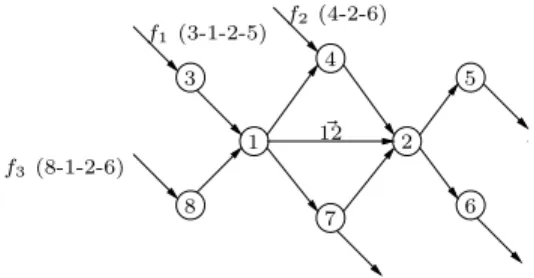
Consider a communication network consisting of a setN
ofnodes connected by a setLoflinks. We consider all links
as unidirectional and denote by`:=ij~, the link from node i ∈ N to nodej ∈ N (cf. Figure 1). Every link `∈ L is characterized by a finite bandwidth B` and a propagation
delay T`.
We assume that the network is being loaded by a setF of
end-to-end flows. Given a flowf ∈ F from nodei∈ N to
nodej∈ N, we denote byrf f-flow’s sending rate, i.e., the rate at which packets are generated and enter nodeiwhere the flow is initiated. Given a link `∈ L in the path of the f-flow, we denote byr`
f the rate at which packets from the f-flow go through the `-link. We call r`
PSfrag replacements 1 2 3 4 5 6 7 8 ~ 12 f1(3-1-2-5) f2(4-2-6) f3(8-1-2-6)
Figure 1: Example network whereq12~ =q f1 ~ 12+q f3 ~ 12.
transmission rate. At each link, the sum of the link/flow
transmission rates must not exceed the bandwidthB`, i.e.,
X
f∈F
r`f ≤B`, ∀`∈ L. (1)
In general, the flow sending ratesrf,f∈ F are determined by congestion control mechanisms and the link/flow trans-mission ratesr`f are determined by packet conservation laws to be derived shortly.
Associated with each link ` ∈ L, there is a queue that temporarily holds packets before transmission. We denote byq`
f the number of bytes in this queue that belong to the f-flow. The total number of bytes in the queue is then given by
q`:=X f∈F
qf`, ∀`∈ L. (2)
The queue can hold, at most, a finite number of bytes that we denote byq`
max. Whenq`reachesq`max, drops will occur.
For each flowf∈ F, we denote byRT Tfthef-flow
round-trip-time that elapses between a packet is sent and its
ac-knowledgment is received. The round-trip-time can also be determined by adding the propagation delaysT`and queu-ing timesq`/B` of all links involved in one round-trip. In particular, RT Tf = X `∈L[f] T`+ q ` B` ,
whereL[f] denotes the set of links involved in one round-trip for flowf.
3.1
Flow conservation laws
Consider a link`∈ Lin the path of flowf∈ F. We denote bys`
f the rate at whichf-flow packets arrive (or originate) at the node where ` starts. We call s`
f the `-link/f-flow
arrival rate. The link/flow arrival rates are related to the
flow sending rates and the link/flow transmission rates by the following simpleflow-conservation law: for everyf∈ F
and`∈ L, s`f :=
(
rf f starts at the node where`starts r`0
f otherwise
(3) where`0denotes the previous link in the path of thef-flow.
For simplicity, we are assuming here single-path routing and unicast transmission. It would be straightforward to de-rive conservation laws for multi-path routing and multi-cast transmission.
3.2
Queue dynamics
In this section, we make two basic assumptions regarding flow uniformity that are used to derive our models for the queue dynamics:
Assumption 1 (Arrival uniformity). On a short
time-interval over which the arrival rates can be assumed approximately constant, the packets of the different flows ar-rive at each node in their paths uniformly distributed over time.
Assumption 2 (Queue uniformity). Packets of the different flows are uniformly distributed in each queue.
Clearly, because of packet quantization, bursting, synchro-nization, etc., these assumptions are never quite true. How-ever, they are sufficiently accurate to lead to models that match closely packet-level simulations. We will show this in Section 4.2.
Consider a link`∈ Lthat is in the path of flowf ∈ F. The queue dynamics associated with this pair link/flow are given by
˙
qf`=s`f −d`f−r`f, where d`
f denotes thef-flow drop rate. In this equations`f should be regarded as an input whose value is determined by upstream nodes. To determine the values of d`f andr`f we consider three cases separately:
1. Empty queue(i.e.,q`= 0). There are no drops and the
outgoing ratesr`f are equal to the arrival ratess`f, as long as the bandwidth constrain (1) is not violated. In case r`
f =s`f,∀f ∈ F would violate (1), the available link bandwidthB`is distributed among all flows pro-portionally to their arrival ratess`
f, which is justified by the Arrival Uniformity Assumption 1. This can be summarized as follows: for everyf∈ F,
d`f = 0, r`f = s` f Pf¯∈Fs`f¯≤B` s` f P ¯ f∈Fs`f¯ B` otherwise
2. Queue neither empty nor full (i.e., 0< q` < qmax` or
q` =q`
max but Pf¯∈Fs`f¯ ≤B`). There are no drops
and because of the Queue Uniformity Assumption 2, the available link bandwidthB` is distributed among the flows proportionally to their percentage of bytes in the queue, i.e., for everyf∈ F,
d`f = 0, rf`= qf` P ¯ f∈Fqf`¯ B`.
3. Queue full and still filling (i.e., q` = qmax` and
P ¯ f∈Fs ` ¯ f > B
`). The total drop rated`must equal the difference between the total arrival rate and the link bandwidth, i.e., d` = P ¯ f∈Fs ` ¯ f −B ` > 0. From the Arrival Uniformity Assumption 1, we conclude that this total drop rated`should be distributed among all flows proportionally to their arrival rates s`f. More-over, from the Queue Uniformity Assumption 2, we conclude that the available link bandwidthB` is dis-tributed among the flows proportionally to their the
percentage of bytes in the queue. This can be summa-rized as follows: for everyf∈ F,
d`f = s`f P ¯ f∈Fs ` ¯ f−B ` P ¯ f∈Fs`f¯ , r`f = q` fB` P ¯ f∈Fq`f¯ . (4)
To complete the queue dynamics model, it remains to determine when and which flows suffer drops. To this ef-fect, suppose that at time t1, q` reached q`max with s` :=
P f∈Fs
`
f > B`. Clearly, a drop will occur at timet1 but, in
general, multiple drops may occur. In general, if a drop oc-curred at timetka new drop is expected at a timetk+1> tk for which the total drop rated`integrates from t
k to tk+1
to the packet-sizeL, i.e., for which z`:= Z tk+1 tk X f∈F d`f = Z tk+1 tk X f∈F s`f−B` =L. (5) We call (5) thedrop-count model.
The question as to which flows suffer drops must be con-sistent (on the average) with the drop rates specified by (4). In particular, the selection of the flowf∗ where a drop
oc-curs is made by drawing the flow randomly from the setF, according to the distribution
pf∗(f) = d`f P ¯ f∈Fd`f¯ = s ` f P ¯ f∈Fs`f¯ , ∀f∈ F. (6)
We assume that the flowsf∗(t
k),f∗(tk+1) where drops occur
at two distinct time instantstk,tk+1are (conditionally)
in-dependent random variables (given that the drops did occur at timestkandtk+1). We call (6) thedrop-selection model.
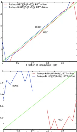
We validated the drop-selection model defined by (6) by matching it withns-2[32] simulations. The top plot in Fig-ure 2 shows the outcome of a simulation where 2 TCP flows (RED and BLUE) compete for bandwidth on a bottleneck queue (with 10% on-off CBR traffic). Thex-axis shows the fraction of arrival rate for each flow and they-axis shows the corresponding drop probability. A 45 degree line would be exactly consistent with (6). We can see in the figure that the probabilities of drop measured experimentally match well with the theoretical 45 degree line.
3.2.1
Hybrid model for queue dynamics
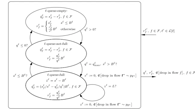
The queue model developed above can be compactly ex-pressed by the hybrid automaton represented in Figure 3. Each ellipse in this figure corresponds to a discrete state (or mode) and the continuous state of the hybrid system con-sists of the flow byte rate s`
f, f ∈ F and the variable z` used to track the number of drops in thequeue-full mode. The differential equations for these variables in each mode are shown inside the corresponding ellipse. The arrows in the figure represent transitions between modes. These tran-sitions are labeled with their enabling conditions (that can include events generated by other transitions), any necessary reset of the continuous state that must take place when the transition occurs, and events generated by the transition. Events are denoted byE[·]. We assume here that a jump al-ways occurs when the transition condition is enabled. This model is consistent with most of the hybrid system frame-works proposed in the literature (cf., e.g., [29]). The inputs to this model are the ratesr`0
f,f∈ Fof the upstream queues
0 0.2 0.4 0.6 0.8 1 0.2 0.4 0.6 0.8 1
Fraction of Incomming Rate
P(drop=BLUE|(B/(R+B))), RTT=90ms P(drop=RED|(R/(R+B))), RTT=45ms BLUE RED 0 0.2 0.4 0.6 0.8 1 0.2 0.4 0.6 0.8 1
Fraction of Incomming Rate
P(drop=RED|(R/(R+B))), RTT=45ms P(drop=BLUE|(B/(R+B))), RTT=90ms
BLUE
RED
Figure 2: Drop probability vs. fraction of arrival rate for 10% background traffic (top) and packet synchronization (bottom).
`0∈ L[`], which determine the arrival ratess`
f,f ∈ F; and the outputs are the transmission rates r`
f,f ∈ F. For the purpose of congestion control, we should also regard the drop events and the queue size as outputs of the hybrid model. Note that the queue sizes will eventually determine packet round-trip-times.
3.2.2
Other drop models
For completeness one should add that the drop-selection model described by (6) is not universal. For example, in dumbbell topologies without background traffic, one can ob-serve synchronization phenomena that sometimes lead to flows with small sending rates suffering more drops than flows with larger sending rates. The bottom plot in Fig-ure 2 shows an extreme example of this (2 TCP flows in a 5Mbps dumbbell topology with no background traffic and drop-tail queuing). In this example, the BLUE flow gets most of the drops, in spite of using a smaller fraction of the bandwidth. In [26], it was suggested that 10% of random delay would remove synchronization for many TCP connec-tions. We used background traffic because this suggested delay is not sufficient when the number of connections is small. The top plot in Figure 2 shows results obtained with background traffic. In the rest of this section, we briefly dis-cuss another drop model that is useful in specific situations. The reader is referred to [4] for additional models.
PSfrag replacements `-queue-empty: ˙ q` f=s ` f−r ` f, f∈ F r` f= s` f s `≤B` s`f s`B ` otherwise `-queue-not-full: ˙ q`f=s`f−r`f, f∈ F r`f= q` f q`B ` `-queue-full: ˙ z`=s`−B` ˙ q`f= (s`f/s`−q`f/q`)B`, f∈ F rf`= q ` f q`B ` q`>0? q`≤0? q`=q` max, s`> B`? s`≤B`? z`:= 0,E drop in flowf∗∼ pf∗ z`=L? z`:= 0,E drop in flowf∗∼ pf∗ dN>0? ( with E[dN] =γ(q`)s`dt) E drop in flowf∗∼pf∗ r`0 f, f∈ F, ` 0 ∈ L[`] q`, r` f,E drop in flowf , f∈ F
Figure 3: Hybrid model for the queue at link`. In this figure, q` is given by (2), thes`f, f∈ F are given by (3), and s`:=P
f∈Fs
`
f, ∀`∈ L.
Drop rotation.
The drop model in (6) is not valid when packet synchronization occurs. This effect is particularly noticeable under TCP congestion control (without cross traffic), when all the flows have the same round-trip time and there is a bottleneck link with bandwidth significantly smaller than that of the remaining links. The corresponding bottleneck queue should be operating under drop-tail [3]. A more accurate model for this situation isdrop rotation. Ac-cording to this model, when the queue gets full each flow gets a drop in a round-robin fashion. The rationale for this is that, once the queue gets full, it will remain full until TCP reacts (approximately one round-trip-time after the drop). In the meanwhile, all TCP flows are in the congestion avoid-ance mode and each will increase its window size by one. When this occurs each will attempt to send two packets back-to-back and, under a drop-tail queuing policy, the sec-ond packet will almost certainly be dropped. Although the drop-count model (5) would predict the correct number of drops, the drop-selection model (6) would not predict drop rotation because of the independence assumption associated with it.3.3
TCP model
So far our discussion focused on the modeling of the trans-mission ratesr`
f and queue sizesq`f across the network, tak-ing as inputs the sendtak-ing rates rf of the end-to-end flows. In this section, we construct a hybrid model for TCP that should be composed with the flow-conservation law and queue dynamics presented in Sections 3.1 and 3.2, in or-der to construct a model that describes the overall system. We start by describing the behavior of TCP in each of its main modes, which we later combine into a hybrid model of TCP. We concentrate here on a single flowf∈ F.
3.3.1
Slow-start mode
Duringslow-start, thecongestion window wf (cwnd) in-creases exponentially, being multiplied by 2 every round-trip timeRT Tf. This can be modeled by
˙ wf =
logm RT Tf
wf, (7)
for an appropriately defined constantm. IfRT Tf was con-stant, we would get
wf(t+RT Tf) =e
logmRt+RT Tf t RT Tf1 dτ
wf(t)≈mwf(t), Sincewf packets are sent each round-trip time, the instan-taneous sending raterf should be given by
rf = wf RT Tf
. (8)
However, in this mode the round-trip time RT Tf tends to increase rapidly because of variations on the queue sizes and therefore this formula needs to be corrected to
rf = βwf RT Tf
, (9)
where the best match with ns-2 traces is obtained for β= 1.45. The formulas (7) and (9) hold as long as the con-gestion windowwf is below the receiver’s advertised window size wadv
f . Whenwf exceeds this value, the sending rate is limited bywadv
f and (9) should be replaced by rf =
min{βwf, wadvf } RT Tf
. (10)
If congestion window reaches the advertised window,
slow-start mode enters congestion-avoidance mode. The
a drop leads the system to thefast-recovery mode, whereas the detection of a timeout leads the system to thetimeout
mode.
3.3.2
Congestion-avoidance mode
During the congestion-avoidance mode, the congestion window size increases “linearly,” with an increase equal to the packet-sizeLfor each round-trip timeRT Tf. This can be modeled by ˙ wf = L RT Tf ,
with the instantaneous sending raterf given by (8). When the receiver’s advertised window size wadv
f is finite, (8) should be replaced by rf = min{wf, wadvf } RT Tf .
Thecongestion-avoidancemode lasts until a drop or timeout
are detected. Detection of a drop leads the system to the
fast-recoverymode, whereas the detection of a timeout leads
the system to thetimeout mode.
3.3.3
Fast-recovery mode
The fast-recovery mode is entered when a drop is
de-tected, which occurs some time after the drop actually oc-curs. When a single drop occurs, the sender leaves this mode at the time it learns that the packet dropped was success-fully retransmitted (i.e., when its acknowledgment arrives). When multiple drops occur, the transition out of fast recov-ery depends on the particular version of TCP implemented. We provide next the model for TCP-Sack and briefly dis-cuss the differences with respect to Reno and TCP-NewReno. Due to lack of space we do not provide here the formal model for the later two versions of TCP.
TCP-Sack.
In TCP-Sack, when ndrop drops occur, thesender learns immediately that several drops occurred and will attempt to retransmit all these packets as soon as the congestion window allows it. As soon as fast-recovery is initiated, the first packet dropped is retransmitted and the congestion window is divided by two. After that, for each ac-knowledgment received, the congestion window is increased by one. However, and until the first retransmission suc-ceeds, the number of outstanding packets is not decreased when acknowledgments arrive.
Suppose that the drop was detected at time t0 and let
wf(t−0) denote the window size just before its division by
2. In practice, during the first round-trip time after the retransmission (i.e., fromt0 to t0+RT Tf) the number of outstanding packets iswf(t−0); the number of duplicate
ac-knowledgments received is equal towf(t−0)−ndrop(we are
in-cluding here the 3 duplicate acknowledgments that triggered the retransmission), and a single non-duplicate acknowledg-ment is received (corresponding to the retransmission). The total number of packets sent during this interval will be one (corresponding to the retransmission that took place im-mediately), plus the number of duplicate acknowledgments received, minus wf(t−0)/2. We need to subtractwf(t−0)/2
because the firstwf(t−0)/2 acknowledgments received will
increase the congestion window up to the number of out-standing packets but will not lead to transmissions because
the congestion window is still below the number of outstand-ing packets [31]. This leads to a total of 1+wf(t−0)/2−ndrop
packets sent, which can be modeled by an average sending rate of rf = 1 +wf(t − 0)/2−ndrop RT Tf on [t0, t0 + RT Tf]. In case a single packet was dropped, fast recovery will finish att0+RT Tf, but otherwise it will continue until all the re-transmissions take place and are successful. However, from t0+RT Tf on, each acknowledgment received will also de-crease the number of outstanding packets so one will observe an exponential increase in the window size. In particular, fromt0+RT Tf tot0+ 2RT Tf the number of acknowledg-ments received is 1+wf(t−0)/2−ndrop(which was the number
of packets sent in the previous interval) and each will both increase the congestion window size and decrease the num-ber of outstanding packets. This will lead to a total numnum-ber of packets sent equal to 2(1+wf(t−0)/2−ndrop) and therefore
rf =2(1 +wf(t
−
0)/2−ndrop)
RT Tf
on [t0+RT Tf, t0+ 2RT Tf]. On each subsequent interval, the sending rate increases ex-ponentially until all thendroppackets that were dropped are
successfully retransmitted. Ink round-trip times, the total number of packets retransmitted is equal to
k−1
X
i=0
2i(1 +wf(t−0)/2−ndrop) =
= (2k−1)(1 +wf(t0−)/2−ndrop),
and the sender will exit fast recovery when this number reachesndrop, i.e., when
(2k−1)(1 +wf(t−0)/2−ndrop) =ndrop ⇔
⇔ k= log2
1 +wf(t−0)/2
1 +wf(t−0)/2−ndrop
. In practice, this means that the hybrid model should remain in the fast recovery mode for approximately
n wf(t−0), ndrop :=llog2 1 +wf(t−0) 2 1 +wf(t − 0) 2 −ndrop m (11) round-trip times. The previous reasoning is only valid when the number of drops does not exceedwf(t−0)/2. As shown in
[31], whenndrop> wf(t−0)/2 + 1 the sender does not receive
enough acknowledgments in the first round-trip time to re-transmit any other packets and there is a timeout. When ndrop =wf(t−0)/2 + 1 only one packet will be sent on each
of the first two round-trip times, followed by exponential in-crease in the remaining round-trip times. In this case, the fast recovery mode will last approximately
n wf(t−0), ndrop:= 1 +dlog2ndrope (12)
round-trip times. The behavior of the several variants of TCP in the presence of multiple packet losses in the same window is also discussed in [7].
In ns-2, the value of the congestion window variable (cwnd) is actually not changed inside the fast-recovery
mode. Instead, a variable (pipe) is used to emulate the con-gestion window of standard TCP-Sack algorithm described
above. For compatibility with ns-2, in our model we ac-tually keep the congestion windowwf constant throughout the whole duration of fast recovery but adjust the sending rates according to the previous formulas.
TCP-NewReno.
TCP-NewReno differs from TCP-Sack in that the sender will only learn about the existence of each additional drop when the retransmission for the previous drop was successful. This means that it must remain in thefast-recoverymode for as many round-trip times as the
num-ber of drops. Thus, our duration of fast recovery increases linear to the number of dropped packets.
TCP-Reno.
In TCP-Reno, the sender leaves thefast-recovery mode as soon as the acknowledgment of the first
retransmitted packet is received, regardless of the occurrence of more drops. In case more drops occur, these will be de-tected right after the fast-recovery mode and the system re-enters fast recovery again. The net result of each time
thefast-recovery mode is entered is a division by two of the
congestion window size. Thus, three dropped packets in a window often leads to a packet timeout [7].
3.3.4
Timeouts
Timeouts occur when the timeout timer exceeds a thresh-old that provides a measure of the current round-trip time. This timer is reset to zero whenever the number of outstand-ing packets decreases (i.e., when it has received an acknowl-edgment for a new packet). Even when there are drops, this should occur at least once everyRT Tf, except in any of the following cases:
1. The number of dropsndropis larger or equal towf−2 and therefore the number of duplicate acknowledg-ments received is smaller or equal to 2. These are not enough to trigger a transition to thefast-recovery
mode.
2. The number of dropsndropis sufficiently large so that
the sender will not be able to exit fast recovery be-cause it does not receive enough acknowledgments to retransmit all the packets that were dropped. As seen above, this corresponds tondrop≥wf/2 + 2.
These two cases can be combined into the following condi-tion under which a timeout will occur:
wf ≤max{2 +ndrop,2ndrop−4}.
When a timeout occurs at timet0 the variablessthrf is set equal to half the congestion window size, which is reset to 1, i.e.,
ssthrf(t0) =w−f(t0)/2, wf(t0) = 1.
At this point, and until w reaches ssthr, we have multi-plicative increase similar to what happens in slow start and therefore (10) hold. This lasts untilwf reachesssthrf(t0) or
a drop/timeout is detected. The former leads to a transition into thecongestion avoidancemode, whereas the latter to a transition into thefast-recovery/timeout mode.
3.3.5
Hybrid model for TCP-Sack
The model in Figure 4 combines the modes described in Sections 3.3.1, 3.3.2, 3.3.3, and 3.3.4 for TCP-Sack. This model also takes into account that there is a delay between
the occurrence of a drop and its detection. This
drop-detection delay is determined by the “round-trip time” from
the queue ` where the drop occurred, all the way to the receiver, and back to the sender. It can be computed by
DDDf` := X `0 ∈L[f,`] T`+ q ` B` ,
where L[f, `] denotes the set of links between the `-queue and the sender, passing through the receiver (for drop-tail queuing, this set should include `itself). To take this de-lay into account, we added two modes (slow-start delayand
congestion-avoidance delay), in which the system remains
between a drop occurs and it is detected. The congestion controller only reacts to the drop once it exists these modes. The timing variablettimis used to enforce that the system
remains in theslow-start delay,congestion-avoidance delay, andfast-recovery modes for the required time. For simplic-ity, we assumed an infinitely large advertised window size in the diagram in Figure 4.
The inputs to the TCP-Sack flow model are the round-trip time, the drop events, and the corresponding drop-detection delays (which can be obtained from the flow-conservation law and queue dynamics in Sections 3.1, 3.2) and its outputs are the sending rates of the end-to-end flows.
The model in Figure 4 assumes that the flowf is always active. It is straightforward to turn the flow on and off by adding appropriate modes (similar to what is done in Section 3.4 for UDP flows). In fact, in the simulation results described in Section 4.2 we used random starting times for the persistent TCP flows.
3.4
UDP model
UDP sources differ from TCP sources in that the former do not perform congestion control. The diagram in Figure 5 represents a simple hybrid model for an on-off UDP source with peak rate equal to rmax and exponential distributions
for the on and the off times with meansτonandτoff,
respec-tively. The average sending rate for this source is given by τonrmax
τon+τoff. This model could be generalized to other
distribu-tions. PSfrag replacements on: rf =rmax ˙ ttim=−1 off: rf= 0 ˙ ttim=−1 ttim<0? ttim<0? ttim∼e − t τoff τoff ttim∼e− t τon τon r` f
Figure 5: Hybrid model for a UDP flow with expo-nential on/off-times.
4.
VALIDATION
We use the ns-2 (version 2.1b9a) packet-level simulator to validate our hybrid models. Different network topologies subject to a variety of traffic conditions are considered.
PSfrag replacements slow-start: ˙ wf =RT Tflogmwf rf=RT Tfβwf slow-start delay: ˙ wf= RT Tflogmwf,ttim˙ =−1 rf=RT Tfβwf cong.-avoidance: ˙ wf=RT TfL rf= RT Tfwf cong.-avoidance delay: ˙ wf= RT TfL ,ttim˙ =−1 rf= RT Tfwf fast-recovery: ˙ wf = 0, t˙tim=−1 ˙ rf= 0 timeout: ˙ ttim=−1 rf= 0 ssthrf :=∞, wf:= 1 E[ndropdrops]? E[ndropdrops]? ttim:=DDD` f ttim:=DDD` f ttim<0? ttim<0? ⊗? ⊗? ⊕ ⊕ ttim<0, k >0? ttim:=RT Tf,k:=k−1,rf:= 2rf ttim<0,k≤0? wf> ssthrf? ttim:=RT Tf ttim<0? E[drop in flowf]? ttim:= 1sec ttim:= 1sec ssthrf:= w− f 2 , wf := 1 ttim<0?
RT Tf,E[ndropdrops (in flowf at queue`)],DDD`f rf
Figure 4: Hybrid model for flow f under TCP-Sack congestion control. The symbol ⊗ stands for wf ≤ max{2 +ndrop,2ndrop−4}and ⊕stands forttim:=RT Tf,k:=n(w−f, ndrop),wf :=
wf− 2 , rf = 1+w−f/2−ndrop RT Tf , wheren(·) is defined by(11)–(12).
4.1
Network Topology
We focus our study on the topologies shown in Figure 6. The topology on the left is known as thedumbbell topology
and is commonly used to analyze TCP congestion control algorithms. The dumbbell topology is characterized by a set of flows that originate at a source node (node 1) and are directed to a sink node (node 2) through abottleneck link. In more realistic networks, a path with several links (and intermediate nodes) would connect the source and destina-tion. However, to analyze congestion control mechanisms, one often ignores the existence of all the intermediate links, except for the bottleneck, i.e., the most congested link.
While the dumbbell topology only considers TCP flows with uniform propagation delays, the flows in the “Y-shape” topology on the right of Figure 6 exhibit distinct propaga-tion delays: 45ms (Src1), 90ms (Src2), 135ms (Src3), 180ms
(Src4). In our simulations, UDP flows make up for the
back-ground traffic injected. Backback-ground flows originate from Src5 and router R2 while TCP flows originate from Src1 to
Src4. The background traffic model we employ is described
in detail in the Section 4.2 below. For the results presented here all queues were chosen to be 40 packets long.
4.2
Simulation Environment
Allns-2simulations use TCP-Sack (more specifically its Sack1 variant outlined in [7]). Each simulation ran for 600 seconds of simulation time and data points were obtained by averaging out 20 trials. TCP flows start randomly between 0 and 2 seconds. We model background traffic as (UDP) on/off CBR flows which turn on/off after being off/on for an exponentially distributed amount of time. We consid-ered different amounts of background traffic in the form of
short-lived flows whose on and off time is 0.5 seconds on av-erage. In particular, the results presented in this paper were obtained by injecting background flows to account for 10% of the traffic. While the exact fraction of short-lived traffic found on the Internet is unknown, it appears that short-lived flows make up for at least 10% of the total Internet traffic [11]. We should point out that the quality of the hybrid system simulations do not degrade as more short-live traffic is considered. As previously mentioned, the drop model is topology dependent. As observed in [3], for the single bot-tleneck topology with uniform propagation delays, drops are deterministic with each flow experiencing drops in a round-robin fashion. However, when background on/off traffic is considered, losses are best modeled stochastically.
The metrics used for comparing the hybrid system and packet-level models include throughput, round trip time, loss rate, and congestion window size for the TCP flows. We also measure queue size at the bottleneck link.
4.3
Results
Figure 7 compares simulation results for the dumbbell topology with a single TCP flow (no background traffic) ob-tained withns-2and our hybrid model. These plots show TCP’s congestion window size and bottleneck queue size over time. As discussed in Section 3.2.2, we use drop ro-tation to model drops in dumbbell topologies. The plots show a nearly perfect match. While most existing models of TCP congestion control are able to capture TCP’s steady-state behavior, TCP slow-start is typically harder to model because it often results in a large number of drops within the same window. We developed our model to capture the basic slow-start behavior of TCP Sack1: When more
PSfrag replacements R1 R2 R1 R2 R3 R4 10ms 5M bps 10ms 5M bps Src1 Src2 Src3 Src4 Src5 Src6 Src1 Src2 Src3 Src4 Src5 Src6 Srcn Srcn Dest1 Dest1 Dest2 Dest2 Dest3 Dest3 Dest4 Dest4 Destn Destn
Figure 6: Dumbbell (left) and Y-shape multi-queue topology with 4 different propagation delays (right).
0 20 40 60 80 100 120 140 0 2 4 6 Queue Size(Packets) Time (seconds) CWND size in Hybrid Model Queue size in Hybrid Model CWND size in NS Queue size in NS 0 20 40 60 80 100 120 140 0 2 4 6 8 10 12 14 16 18 20 Queue Size(Packets) Time (seconds) CWND size in Hybrid Model Queue size in Hybrid Model CWND size in NS Queue size in NS
Figure 7: Comparison of the congestion window and queue sizes over time for the dumbbell topology with one TCP flow and no background traffic.
than cwnd/2+1 packets are lost, a timeout occurs because there are not enough acknowledgments to open the conges-tion window [31]; and when the number of losses is around cwnd/2, Sack1 eventually leaves fast-recovery but only after a few multiples of the round-trip time (cf. Section 3.3.3). This is consistent with Figure 7, where we see that, after the initial drops, the congestion window is divided by two and maintains this value for about half a second before it begins increasing linearly.
In the next set of experiments, we simulate 4 TCP flows on the dumbbell topology with and without background traffic. Figure 8 shows the simulation results without background traffic. As observed in previous studies, TCP connections with the same RTT get synchronized and this synchroniza-tion persists even for a large number of connecsynchroniza-tions [34, 26]. This synchronization is modeled using drop rotation. Similarly to the single flow case, the two simulations coin-cide almost exactly. Specifically, in steady state, all flows synchronize to a saw-tooth pattern with period around 1 second. 0 20 40 60 80 100 120 140 0 2 4 6 8 10 12 14 16 18 20
Cwnd and Queue Size(Packets)
Time (seconds) CWND size of TCP1 CWND size of TCP2 CWND size of TCP3 CWND size of TCP4 Queue size of Q1 0 20 40 60 80 100 120 140 0 2 4 6 8 10 12 14 16 18 20
Cwnd and Queue Size(Packets)
Time (seconds) CWND size of TCP1 CWND size of TCP2 CWND size of TCP3 CWND size of TCP3 Queue size of Q1
Figure 8: Congestion window and queue size over time for the dumbbell topology with 4 TCP flows and no background traffic. Simulations using ns-2
(top) and a hybrid model (bottom).
Simulation results for 4 TCP flows with background traffic are summarized in Table 1, which presents average through-put and round-trip time for each flow for both hybrid system andns-2simulations. These statistics confirm that the hy-brid model nearly reproduces the results obtained from the packet-level model.
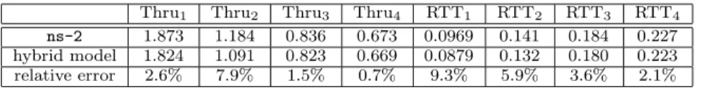
To validate our hybrid models, we also use the Y-shape, multi-queue topology with different round-trip-times shown on the right-hand side of Figure 6. As discussed in Sec-tion 3.2, we consider the drop-count and drop-selecSec-tion mod-els described by Equations (5) and (6), respectively. Unlike in the drop rotation model in which losses are deterministic, (6) generates stochastic drops. Since losses are random, no two simulations will be exactly the same so it is not pos-sible for the hybrid model to exactly reproduce the results fromns-2. Table 2 summarizes simulation results obtained withns-2and the hybrid model for 4 TCP flows with 10% background traffic on the Y-shape topology under drop tail discipline. This table presents the mean throughput and
Thru1 Thru2 Thru3 Thru4 RTT1 RTT2 RTT3 RTT4
ns-2 1.14 1.13 0.13 1.12 0.094 0.094 0.094 0.094
hybrid system 1.14 1.15 1.15 1.15 0.096 0.096 0.096 0.096 relative error 0% 0.01% 0.01% 0.02% 0.02% 0.02% 0.02% 0.02%
Table 1: Average throughput and round-trip time for the dumbbell topology with 4 TCP flows and 10% background traffic.
mean round-trip time for each competing TCP flow. Note that the relative error is less than 10% and in most cases well under 10%. Similar results hold for variations of the Y-shape topology, e.g., different round-trip times, number of competing flows. However, for the stochastic drop model to hold, there must be either background traffic and/or enough complexity in the topology and flows such that synchroniza-tion does not occur. When synchronizasynchroniza-tion does occur, then a deterministic model for drops should be employed. As described in Section 3.2.2, in single bottleneck topologies drop-rotation provides an accurate model. However, in more complex settings, deriving the deterministic drop model is quite challenging. This is one direction of future work we plan to pursue.
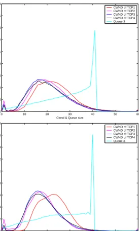
A more accurate methodology to compare stochastic pro-cesses is to examine their probability density function. Fig-ure 9 plots the probability density functions corresponding to the time-series used to generate the results in Table 2. We observe that the hybrid model can reproduce similar probability densities. Regarding the density function of the congestion window, three of the flows closely agree, while one shows a slight bias towards the larger value. The den-sity function of the queue is similar for both models. One noticeable discrepancy is that the peak near the queue-full state is sharper in the case of the hybrid model. This dif-ference is due to the fact that the queue in ns-2can only take integer values, while the queue in the hybrid model can take fractional values. Thus, the probability that the queue is nearly full is represented by a probability mass atqmax−ε
for the hybrid model, while it is represented by probability mass atqmax−1 in ns-2. This results in a more smeared
probability mass around queue-full in the case of ns-2. While visually comparing two density functions provides a general understanding of their similarity, there are sev-eral quantitative metrics to compare density functions. One good metric is theL1-distance [6], which has the desirable
property that whenf andgare densities,
R f−g = 2 supA R Af− R Ag .
Thus, if the probability of an eventAis to be predicted, the error of the prediction is half of theL1-distance between the
density functions. Table 3 shows theL1-distance between the hybrid model and ns-2histograms. The distances in-dicate that the hybrid model provides a good prediction of the actual probability density function.
5.
COMPUTATIONAL COMPLEXITY
While hybrid systems allow for a theoretical understand-ing of networks, they are also amenable to simulation.
In [18] it was shown that a ripple effect may greatly de-grade the efficiency of fluid models. Since a hybrid model is to some extent a fluid model, one might expect an increase
0 10 20 30 40 50 60 0 0.02 0.04 0.06 0.08 0.1 0.12 0.14 0.16 0.18
Cwnd & Queue size
P CWND of TCP1 CWND of TCP2 CWND of TCP3 CWND of TCP4 Queue 3 0 10 20 30 40 50 60 0 0.02 0.04 0.06 0.08 0.1 0.12 0.14 0.16 0.18
Cwnd & Queue size
P CWND of TCP1 CWND of TCP2 CWND of TCP3 CWND of TCP4 Queue 3
Figure 9: Probability density functions for the con-gestion window and queue size for the Y-shape topology with 4 TCP flows and 10% background traffic. These were computed from simulations us-ing ns-2(top) and a hybrid model (bottom).
in computation speed when compared to a packet level sim-ulator such as ns-2. However, in [18] the flow rates are held constant between events, whereas here we utilize ordi-nary differential equations (ODEs) to describe the bit-rates, accommodating complex variations in the sending rates be-tween events.
Modern ODE solvers are especially efficient while the con-tinuous variables are well modeled by polynomials. How-ever, in networks the bit-rates have occasional discontinu-ities. This requires special care and can lead to signifi-cant computational burden. In fact, the simulation time grows essentially linearly with the number of discontinuities in the continuous variables. In our models, these discontinu-ities are essentially caused by two types of discrete events: drops and queues emptying. Drops typically cause TCP to abruptly decrease the congestion window, whereas a queue
Thru1 Thru2 Thru3 Thru4 RTT1 RTT2 RTT3 RTT4
ns-2 1.873 1.184 0.836 0.673 0.0969 0.141 0.184 0.227
hybrid model 1.824 1.091 0.823 0.669 0.0879 0.132 0.180 0.223 relative error 2.6% 7.9% 1.5% 0.7% 9.3% 5.9% 3.6% 2.1%
Table 2: Average throughput and round-trip time for the Y-shape topology with 4 TCP flows and 10% background traffic.
cwnd1 cwnd2 cwnd3 cwnd4 bottleneck queue 4 flows dumbbell with background traffic 0.0071 0.0067 0.0071 0.0066 0.0108 4 flows y-shape with background traffic 0.0034 0.0044 0.0025 0.0033 0.0054
Table 3: L1-distance between histograms computed from simulations usingns-2 and a hybrid model.
becomes empty forces the outgoing bit-rates to switch from a fraction of the outgoing link bandwidth to the incoming bit-rates1. It turns out that the frequencies at which these events occur are essentially determined by the drop-rates of the active flows and the rate at which flows start and stop. These issues are illustrated in the comparison in Table 4 betweenns-2and an hybrid model. This table shows exe-cution time (in seconds) of ns-2 and the hybrid simulator Modelica [23], where a single bottleneck topology with 20ms propagation delay was utilized. The bandwidth of the bot-tleneck link is 5Mbps, 50Mbps or 500Mbps as shown. There were either one or three long-lived TCP flows competing for the bottleneck bandwidth. Each simulation ran for 10 min-utes of simulations time. The table displays the number of seconds required to complete the simulation on a 1.2GHz Pentium PC with 512MB memory.
Since the main factor that determines the simulation speed is the drop-rate, it is informative to study how it scales with the number of flows. To this effect consider the well-known equation T = RT Tc√p, which relates the per-flow throughputT, the average round-trip time RT T, and the drop probabilitypfor dumbbell topology [24]. Ac-cording to this formula the total drop-rate forncompeting flows, which is equal tonT p, is given by n
T c2
RT T2. This
sug-gests that the computational complexity is of orderO(n/T), scaling linearly with the number of flows when the per-flow throughput is maintained constant and is actually inversely proportional to the per-flow throughput when the number of flows remains constant. This is in sharp contrast with event-based simulators for which the computational complexity is essentially determined by the total number of packets trans-mitted, of orderO(nT). This is confirmed by the results in Table 4, which show that the hybrid simulator is especially competitive for large per-flow throughputs. However, when many flows share a low-bandwidth link packet-level simula-tors have the advantage. E.g., when 3 flows share a 5Mbps linkns-2is only twice as slow and could actually be faster than our hybrid simulator if we increased the number of flows.
Memory usage is also a concern when simulating networks. Hybrid systems requires one state variable for each active flow and one state variable for each flow passing through a
1Neither of these events exhibits the type of explosion
de-scribed in [18] because none of them instantaneously gener-ates further events of the same type downstream. Actually, a queue emptying can eventually cause other queues to empty downstream but not before some time has elapsed.
queue. Hence, memory usage scales linearly with the num-ber of flows and numnum-ber of queues. Forns-2, the memory usage depends on the number of packets in the system, and hence scales with the bandwidth delay product.
6.
CONCLUSION AND FUTURE WORK
We propose a general framework for building hybrid mod-els that describe network behavior. Our hybrid systems framework fills the gap between packet-level and aggregate models by averaging discrete variables over a very short time scale. This means that the model is able to capture the dy-namics of transient phenomena fairly accurately, as long as their time constants are larger than a couple of round-trip times. This is quite appropriate for the analysis and de-sign of network protocols including congestion control mech-anisms.
One direction for future research is to perform very large scale simulation. We found that the hybrid model accurately matches discrete packet level simulation for small simula-tions. However, the real benefit of this approach will be-come apparent after a study of very large scale simulations is complete.
7.
REFERENCES
[1] J. S. Ahn and P. B. Danzig. Packet network simulation: speedup and accuracy versus timing granularity.IEEE/ACM Trans. on Networking, 4(5):743–757, Oct. 1996.
[2] S. Bohacek. Fair pricing of video transmissions using best-effort and purchased bandwidth. InProc. of the 40th Annual Allerton Conf. on Comm., Contr., and
Computing, 2002.
[3] S. Bohacek, J. P. Hespanha, J. Lee, and K. Obraczka. Analysis of a TCP hybrid model. InProc. of the 39th Annual Allerton Conf. on Comm., Contr., and
Computing, Oct. 2001.
[4] S. Bohacek, J. P. Hespanha, J. Lee, and K. Obraczka. A hybrid systems modeling framework for fast and accurate simulation of data communication networks: Extended version. Technical report, University of California, Santa Barbara, Nov. 2002.
[5] N. Cardwell, S. Savage, and T. Anderson. Modeling TCP latency. InProc. of the IEEE INFOCOM, Tel-Aviv, Israel, Mar. 2000.
[6] L. Devroye.A Course in Density Estimation. Birkhauser, Boston, 1987.
1 TCP (5M) 3 TCPs (5M) 1 TCP (50M) 3 TCPs (50M) 1 TCP (500M) 3 TCPs (500M) Hybrid model 0.37 2.78 0.15 0.511 .87 1.39
ns-2 5.4 5.5 107 107 978 1094
Table 4: Execution time (in seconds) of ns-2 and Modelica for 10 minutes of simulation time.
[7] K. Fall and S. Floyd. Simulation-based comparisons of Tahoe Reno and SACK TCP.ACM
Comput. Comm. Review, 27(3):5–21, July 1996.
[8] S. Floyd. Connections with multiple congested gateways in packet-switched networks part1: One-way traffic.ACM Comput. Comm. Review, 21(5):30–47, Oct. 1991.
[9] S. Floyd, M. Handley, J. Padhye, and J. Widmer. Equation-based congestion control for unicast applications. InProc. of the ACM SIGCOMM, pages 43–56, Aug. 2000.
[10] Y. Guo, W. Gong, and D. Towsley. Time-stepped hybrid simulation (TSHS) for large scale networks. In
Proc. of the IEEE INFOCOM, Mar. 2000.
[11] F. Hern´andez-Campos, J. S. Marron,
G. Samorodnitsky, and F. D. Smith. Variable heavy tail duration in Internet traffic,. InProc. of
IEEE/ACM MASCOTS 2002, 2002.
[12] H. Hisamatsu, H. Ohsaki, , and M. Murata. On modeling feedback congestion control mechanism of TCP using fluid flow approximation and queuing theory. InProc. of 4th Asia-Pacific Symp. on
Information and Telecommunication Technologies,
2001.
[13] P. Huang, D. Estrin, and J. Heidemann. Enabling large-scale simulations: selective abstraction approach to the study of multicast protocols. InProc. of the Int. Symp. on Modeling, Analysis and Simulation of
Computer and Telecommunication Systems, pages
241–248. IEEE, July 1998.
[14] G. Kesidis, A. Singh, D. Cheung, and W. Kwok. Feasibility of fluid-event-driven simulation for ATM networks. InProc. IEEE GLOBECOM, volume 3, pages 2013–2017, Nov. 1996.
[15] K. Kumaran and D. Mitra. Performance and fluid simulations of a novel shared buffer management system. InProc. of the IEEE INFOCOM, pages 1449–1461, Mar. 1998.
[16] S. Kunniyur and R. Srikant. Analysis and design of an adaptive virtual queue (AVQ) algorithm for active queue management. InProc. of the ACM SIGCOMM, San Diego, California, USA, 8 2001.
[17] T. V. Lakshman, U. Madhow, and B. Suter.
Window-based error recovery and flow control with a slow acknowledgment channel: A study of TCP/IP performance. InProc. of the IEEE INFOCOM, Apr. 1997.
[18] B. Liu, D. R. Figueiredo, J. K. Yang Guo, and D. Towsley. A study of networks simulation efficiency: Fluid simulation vs. packet-level simulation. In
Proc. of the IEEE INFOCOM, volume 3, pages
1244–1253, Apr. 2001.
[19] S. H. Low, F. Paganini, J. Wang, S. Adlakha, and J. C. Doyle. Dynamics of TCP/RED and a scalable control. InProc. of the IEEE INFOCOM, June 2002.
[20] M. Mathis, J. Semke, J. Mahdavi, and T. Ott. The macroscopic behavior of the TCP congestion avoidance algorithm. ACM Comput. Comm. Review, 27(3), July 1997.
[21] V. Misra, W. Gong, and D. Towsley. Stochastic differential equation modeling and analysis of TCP-windowsize behavior. InProc. of
PERFORMANCE’99, Istanbul, Turkey, 1999.
[22] V. Misra, W. Gong, and D. Towsley. Fluid-based analysis of a network of AQM routers supporting TCP flows with an application to RED. InProc. of the
ACM SIGCOMM, Sept. 2000.
[23] Modelica Association.Modelica — A Unified Object-Oriented Language for Physical Systems
Modeling: Tutorial.Available at
http://www.modelica.org/.
[24] T. Ott, J. H. B. Kemperman, and M. Mathis. Window size behavior in TCP/IP with constant loss
probability. InProc. of the DIMACS Workshop on
Performance of Realtime Applications on the Internet,
Nov. 1996.
[25] J. Padhye, V. Firoiu, D. Towsley, and J. Kurose. Modeling TCP throughput: a simple model and its empirical validation. InProc. of the ACM SIGCOMM, Sept. 1998.
[26] L. Qiu, Y. Zhang, and S. Keshav. Understanding the performance of many TCP flows.Computer Networks, 37:277–306, Nov. 2001.
[27] QualNet user manual. Available at
http://www.scalable-networks.com.
[28] Scalable simulation framework. Available at
http://www.ssfnet.org/.
[29] A. V. D. Schaft and H. Schumacher.An Introduction
to Hybrid Dynamical Systems. Number 251 in
Lect. Notes in Contr. and Inform. Sci. Springer-Verlag, London, 2000.
[30] D. Schwetman. Hybrid simulation models of computer systems. Communications of the ACM, 19:718–723, Sept. 1978.
[31] B. Sikdar, S. Kalyanaraman, and K. Vastola. Analytic models for the latency and steady-state throughput of TCP Tahoe, Reno and SACK. InProc. of IEEE
GLOBECOM, pages 25–29, 2001.
[32] The VINT Project, a collaboration between
researchers at UC Berkeley, LBL, USC/ISI, and Xerox PARC.The ns Manual (formerly ns Notes and
Documentation), Oct. 2000. Available at
http://www.isi.edu/nsnam/ns/ns-documentation.html.
[33] A. Yan and W. Gong. Fluid simulation for high speed networks.IEEE Trans. on Inform. Theory, June 1999. [34] L. Zhang, S. Shenker, and D. D. Clark. Observations
on the dynamics of a congestion control algorithm: The effects of two-way traffic. InProc. of the ACM