for Statistical Tests and Bayesian Inference
Wittawat Jitkrittum
A dissertation submitted in partial fulfillment of the requirements for the degree of
Doctor of Philosophy of
University College London.
Gatsby Computational Neuroscience Unit University College London
Declaration
I, Wittawat Jitkrittum, confirm that the work presented in this thesis is my own. Where information has been derived from other sources, I confirm that this has been indicated in the thesis.
Abstract
The kernel mean embedding is known to provide a data representation which pre-serves full information of the data distribution. While typically computationally costly, its nonparametric nature has an advantage of requiring no explicit model specification of the data. At the other extreme are approaches which summarize data distributions into a finite-dimensional vector of hand-picked summary statistics. This explicit finite-dimensional representation offers a computationally cheaper alternative. Clearly, there is a trade-off between cost and sufficiency of the representation, and it is of interest to have a computationally efficient technique which can produce a data-driven representation, thus combining the advantages from both extremes.
The main focus of this thesis is on the development of linear-time mean-embedding-based methods to automatically extract informative features of data distributions, for statistical tests and Bayesian inference. In the first part on statistical tests, several new linear-time techniques are developed. These include a new kernel-based distance measure for distributions, a new linear-time nonparametric dependence measure, and a linear-time discrepancy measure between a probabilistic model and a sample, based on a Stein operator. These new measures give rise to linear-time and consistent tests of homogeneity, independence, and goodness of fit, respectively. The key idea behind these new tests is to explicitly learn distribution-characterizing feature vectors, by maximizing a proxy for the probability of correctly rejecting the null hypothesis. We theoretically show that these new tests are consistent for any finite number of features. In the second part, we explore the use of random Fourier features to construct approximate kernel mean embeddings, for representing messages in expectation propagation (EP) algorithm. The goal is to learn a message operator which predicts EP outgoing messages from incoming messages. We derive a novel two-layer random feature representation of the input messages, allowing online learning of the operator during EP inference.
Acknowledgements
I would like to express my deep gratitude to my supervisor, Arthur Gretton, for his excellent supervision throughout my study. Arthur has always patiently listened to and helped solve problems I encountered. I thank the Gatsby Charitable Foundation for the financial support of my PhD study. I am grateful to Mijung Park and Zoltán Szabó for being a great collaborator over the years. I thank Zoltán Szabó’s patience and kindness for mentoring me. I am grateful to Kenji Fukumizu for hosting me when I visited the Institute of Statistical Mathematics, and for fruitful research discussions. I thank all Gatsby Unit’s members for intellectually stimulating discussions in the afternoon tea times. I thank my officemates: Carsen Stringer, Vincent Adam, Federico Mancinelli, Sanjeevan Ahilan, Kevin Wenliang Li, and Wenkai Xu, who have listened and responded to my complaints, and chatted about random scientific ideas with me. I thank Barry Fong for providing interesting stimulating questions from the perspective of a non-researcher. I thank my family for their love and support. A special thank goes to Jiamin Su who provided me emotional support in my final year.
Contents
1 Introduction 11
1.1 Informative Features for Statistical Tests . . . 11
1.2 Informative Features for Learning to Infer . . . 14
1.3 Structure of the Thesis . . . 15
2 Kernel Methods for Learning on Distributions 17 2.1 Reproducing Kernel Hilbert Space . . . 17
2.2 Kernel Mean Embedding . . . 20
2.3 Maximum Mean Discrepancy . . . 20
2.3.1 Characteristic Kernels . . . 21
2.3.2 Estimation, Convergence, and Asymptotic Distributions . . . 22
2.4 Applications of Mean Embedding . . . 23
2.5 Properties of Kernels . . . 25
3 Informative Features for Distinguishing Distributions 29 3.1 Introduction . . . 29
3.2 Mean Embedding (ME) Test . . . 31
3.2.1 Unnormalized ME Statistic . . . 31
3.2.2 Normalized ME (NME) Statistic . . . 33
3.3 Smooth Characteristic Function (SCF) Test . . . 33
3.4 Proposal: Interpretable Two-Sample Tests . . . 35
3.4.1 A Test Power Lower Bound and Feature Learning . . . 35
3.4.2 Convergence of the Normalized ME Test Power Criterion . . . . 38
3.5 Experiments . . . 39
3.5.1 Informative Features: Simple Demonstration . . . 40
3.5.2 Test Power Vs. Sample Sizen . . . 41
3.5.3 Test Power Vs. Dimensiond . . . 42
3.5.4 Distinguishing Articles From Two Categories . . . 43
3.5.5 Distinguishing Positive and Negative Emotions . . . 44
3.6 Runtimes . . . 46
3.7 Preprocessing of the NIPS Text Collection . . . 47
Proofs. . . 49
3.A Proof: Convergence of the NME Power Criterion . . . 49 7
3.A.1 Bound in Terms of Snandzn . . . 51
3.A.2 Empirical Process Bound on ¯zn . . . 52
3.A.3 Empirical Process Bound onSn. . . 53
3.A.4 Bounding by Concentration and the VC Property . . . 55
3.A.5 Finite VC Index of the Gaussian Kernel Class . . . 57
3.B Proof: A Lower Bound on the Test Power . . . 58
3.C External Lemmas . . . 61
4 Informative Features for Dependence Detection 63 4.1 Introduction . . . 63
4.2 New Statistic: The Finite Set Independence Criterion (FSIC) . . . 65
4.3 Normalized FSIC and Adaptive Test . . . 69
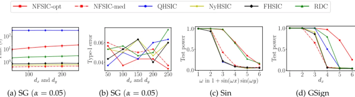
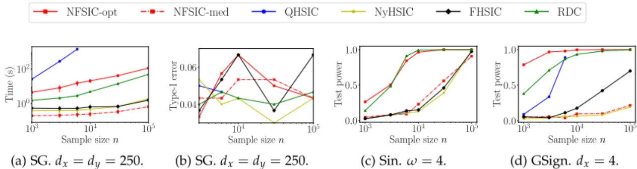
4.4 Experiments . . . 73
4.4.1 Toy Problems . . . 74
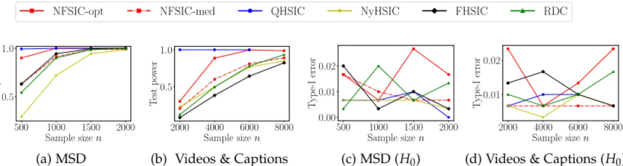
4.4.2 Real Problems . . . 76
4.4.3 Redundant Test Locations . . . 78
4.4.4 Test Power Vs. Number J of Test Locations . . . 78
Proofs. . . 81
4.A Proof: A Lower Bound on the Test Power . . . 81
4.B Helper Lemmas . . . 90
5 Informative Features for Model Criticism 93 5.1 Introduction . . . 93
5.2 Kernel Stein Discrepancy (KSD) Test . . . 95
5.3 New Statistic: The Finite Set Stein Discrepancy (FSSD) . . . 96
5.3.1 Goodness-of-Fit Test with the FSSD Statistic . . . 98
5.3.2 Optimizing the Test Parameters . . . 99
5.4 Relative Efficiency of the FSSD and LKS Tests . . . 101
5.4.1 Relative Efficiency and Bahadur Slope . . . 101
5.4.2 Approximate Bahadur Slopes ofnFSSDd2and√nSb2 l . . . 103
5.5 Experiments . . . 108
5.5.1 Sensitivity to Local Differences . . . 108
5.5.2 Test Power . . . 108
5.5.3 Informative Features . . . 112
5.5.4 Rejection Rate Vs. Number J of Test Locations . . . 113
5.6 Known Results . . . 114
6 Informative Features for Automated Expectation Propagation 115 6.1 Introduction . . . 115
6.2 Message Passing . . . 117
6.2.1 Belief Propagation and Expectation Propagation . . . 118
6.2.2 Expectation Propagation . . . 119
6.2.4 Learning to Pass EP Messages . . . 121
6.3 Proposal: Kernel-Based Message Operators . . . 123
6.3.1 Kernels on Tuples of Distributions . . . 123
6.3.2 Random Feature Approximations . . . 124
6.3.3 Regression for Message Prediction . . . 126
6.4 Experiments . . . 127
Supplementary . . . 135
6.5 Median Heuristic for the Gaussian Kernel on Mean Embeddings . . . . 135
6.6 Kernels and Random Features . . . 136
6.6.1 Random Features . . . 136
6.6.2 MV (Mean-Variance) Kernel . . . 136
6.6.3 Expected Product Kernel . . . 137
6.6.4 Product and Sum Kernels on Mean Embeddings . . . 138
6.7 More Details on Experiment 1: Batch Learning . . . 139
7 Conclusions and Future Work 141 A Appendix 143 A.1 U-Statistics . . . 143
Introduction
We address the problem of finding computationally efficient, and informativefeatures of data distributions, while making as few assumptions as possible on the underly-ing generatunderly-ing distributions. We consider two different contexts: 1) nonparametric statistical tests for comparing distributions, and 2) approximate Bayesian inference.
1.1
Informative Features for Statistical Tests
The task of nonparametric comparison of distributions is broad, and encompasses long-standing problems such as two-sample testing, independence testing, and goodness-of-fit testing. These will be the three problems that we consider in the first part. The three problems can be rephrased as finding the differences between two distributionsPand Q by testing the null hypothesis H0: P = Q against the alternative H1: P 6= Q for
some distributionsPandQ. Two-sample testing aims to testH0: P=Qon the basis
of two samples drawn from the two unknown distributionsPandQ. Independence testing tests statistical dependence of two random vectors X and Y. Equivalently, this can be cast as testing H0: Pxy = PxPy using only the joint sample drawn from
the unknown joint distribution Pxy, where Px and Py are the respective marginal
distributions ofXandY. Goodness-of-fit testing examines whether a given sample follows a known probability distribution (model): given a sample from an unknown distributionQ, and a known modelP, it testsH0: P= Q. The knowledge ofPis what
distinguishes goodness-of-fit testing from the two-sample testing.
We consider only nonparametric testing, meaning that the assumptions made on the distributionsPand Qare mild. Importantly, we do not assume any parametric family to whichPandQbelong, in any of the three problems. By contrast, the well known t-test can be seen as a form of restrictive two-sample test, where the two samples are represented by their empirical means. In this case, the difference between PandQcan be detected only when there is a difference between the means, a strong implicit assumption which may not hold in practice. Many modern nonparametric tests are based on the use of positive definite kernels whose corresponding reproducing kernel Hilbert spaces (RKHSs) are of infinite dimensional [Gretton et al., 2005b,c, Moulines et al.,2008,Gretton et al.,2012a,Chwialkowski et al.,2014,Chwialkowski
and Gretton,2014,Chwialkowski et al.,2015,2016]. The central idea is based on the representation of empirical distributions with the so called kernel mean embeddings [Berlinet and Thomas-Agnan,2004,Smola et al.,2007].
Given a distributionP, its mean embedding is defined as the expectation of the feature map implicitly defined by the kernel, resulting in a representation ofPas a point in the RKHS. It can shown that if the kernel ischaracteristic[Sriperumbudur et al., 2011], then the mean map is injective, so that the distance between two distributions as measured in the embedded RKHS defines a distance in the original space of distri-butions. The use of such RKHS distance has led to the maximum mean discrepancy (MMD) test [Gretton et al., 2006, 2012a], a modern state-of-the-art nonparametric two-sample test. Measuring the distance betweenPxy andPxPy by the MMD leads to
the so called Hilbert Schmidt Independence Criterion (HSIC) [Gretton et al.,2005a,b] which can be used to construct a consistent independence test. For goodness-of-fit testing, to the best of our knowledge, a multivariate, nonparametric (i.e., the model Pis not restricted to a parametric family) test has not been studied in the literature until the recent works of Liu et al.[2016] andChwialkowski et al.[2016]. The tests in these two works rely on a kernelized Stein operator to define the test statistic. Briefly, these tests rely on a test statistic given by the empirical expectation under Q of aP-dependent function (constructed by a Stein operator of P). It was shown that asymptotically the expectation of such a function is zero if and only if the sample follows P, allowing one to conduct a nonparametric goodness-of-fit test without the need of a sample from P. Further, the dependency onPin the constructed function is only through the gradient (with respect to the input variable) of the log density. This means that the normalizer ofPdoes not need to be known, and the test can be applied to a complex model whose normalizer may be computationally intractable. Motivations and Contributions Despite strong theoretical properties, a bottleneck common to all the kernel-based tests is their high runtime complexity, which is quadratic in the sample size. This high cost means that these tests can be applied to only problems of small size. In the followings, we briefly describe three commonly used techniques to reduce the computation.
1. Random Fourier Features [Rahimi and Recht, 2007, Zhao and Meng, 2014, Zhang et al.,2017]: this approach aims to approximate evaluation of the kernel with a dot product in a finite-dimensional space, constructed by randomly sampling from the spectral density of the kernel. The test statistic can then be rewritten in its “primal form” so that the dominant term in the computational complexity is the number of features, rather than the sample size. While this approach allows the test to be applied to larger problems, the use of a finite-dimensional kernel implies that the test is no longer consistent. That is, since only finitely many statistics can be captured, there exists a pair of P,Q that cannot be distinguished by the test. To ensure test consistency, as sample size increases, a growing number of features is needed. However, this defeats the
purpose of reducing the runtime in the first place.
2. Incomplete Cholesky Factorization and Nyström Method[Williams and Seeger, 2001,Zhang et al.,2017]: incomplete Cholesky factorization and the Nyström method approximate the kernel Gram matrix with a low-rank factorization by taking advantage of the fact that the kernel has a rapidly decaying spectrum (e.g., the Gaussian kernel). The test statistic can be rewritten in terms of the low-rank factors of the Gram matrix, thus reducing the computation. The asymptotics and consistency of a test based on the Nyström method or incomplete Cholesky factorization remain a challenging open question. Further, when the kernel spectrum does not decay sufficiently rapidly, the reduced rank may still need to be large to accurately approximate the Gram matrix.
3. Incomplete U-Statistic[Gretton et al.,2012a,Zaremba et al.,2013,Zhang et al., 2017]: many kernel-based test statistics can be written as a second-order U-statistic (Section A.1: U-Statistics), taking the form Tn = n(n2−1)∑i<jh(zi,zj)
for some function h, where n is the sample size, and {zi}ni=1 is the observed
sample. Computational complexity of TnisO(n2). The idea of an incomplete
U-statistic is to subsample summands in Tnso that the number of terms left is
of order O(n). The result is a test statistic which can be computed in linear-time, and is still unbiased. An advantage over the previous two approaches is that test consistency still remains (if the originalTn yields a consistent test).
A disadvantage is that it tends to give a test with low test power (i.e., the probability of rejecting H0 when it is false) for finiten, due to the increase in the
variance of the statistic.
An equally pressing issue is the choice of the kernel itself. Of all the aforementioned kernel tests, apart from the MMD two-sample test for which kernel optimization has been investigated [Gretton et al.,2012b,Sutherland et al.,2016], there is no principled way of optimizing kernels in the HSIC test of independence, and the kernelized Stein test of goodness of fit. These are the motivations for our proposals. Our goals are to develop new kernel tests for the three types of testing which address the drawbacks of existing kernel tests, while maintaining their advantages:
1. The new tests have a principled way of choosing kernels and all other hyperpa-rameters.
2. The new tests, including the parameter tuning procedure, run in linear-time (with respect to the sample size).
3. The new tests can be used with multivariate random variables, are nonparametric and consistent.
The key idea behind these new tests is to learn explicit features (points in the same domain as the input data) so as to maximize the rate of detecting the differences between the two distributions i.e., the test power. The features not only allow one to
avoid the expensive (quadratic in the sample size) computation of the distance in the RKHS, but turn out to also pinpoint and indicate where the two distributions differ. For instance, in the goodness-of-fit test, the latter property makes the test interpretable: it uniquely gives evidence indicating the region in which the modelPfails to fit the data. All hyperparameters can be automatically tuned so as to maximize the (lower bound on the) test power. This series of works thus simultaneously addresses a number of long-standing issues in kernel-based hypothesis testing, namely, unavailability of a parameter tuning procedure, and high runtime complexity. Importantly, our linear-time tests are consistent forany finite number of features. To reiterate, the commonly used random Fourier features [Rahimi and Recht,2007] to speed up kernel-based tests requires a growing number of features to guarantee test consistency.
Our new two-sample test, independence test, and goodness-of-fit test are described in Chapter3, Chapter4, and Chapter5, respectively.
1.2
Informative Features for Learning to Infer
Given a graphical model consisting of factors (non-negative functions e.g., condi-tional probability densities) capturing how neighboring variables interact, the goal of Bayesian inference is to infer the posterior distribution of some variables of interest, conditioning on observed realizations of others. A commonly used approximate inference scheme is expectation propagation (EP), which recursively passes evidence from the observed variables in the form of outgoing messages (i.e., functions or distri-butions), to the variables to be inferred. Each message can be computed locally at a factor as a function of incoming messages from the neighbors.
Goals A major challenge is that computing a message typically involves an intractable integral over a complicated factor, and may require an expensive numerical integra-tion. A typical approach is to manually compute (or approximate) the integral for each considered factor, and implement accordingly in the inference engine. This is the approach taken by Infer.NET [Minka et al., 2014], a probabilistic programming framework which supports EP. While the modeler can freely compose their model from supported factors known to the inference engine, using a customized factor still requires manual implementation of the outgoing messages. Our goal is to automate the computation of outgoing messages in EP for arbitrary factors, so that no manual derivation is needed. Further, we also require that the overhead resulting from such automation be kept minimal.
An approach due toBarthelmé and Chopin [2011] is to compute the messages via importance sampling. Although this approach eliminates the need of manual derivation of message computation, it suffers from high computational complexity. Heess et al.[2013] use neural networks to predict outgoing messages from incoming messages, replacing the expensive numerical integration. The neural networks are trained offline on importance sampled instances of incoming/outgoing message pairs. While there is a large gain in runtime, this approach requires training data that cover
the relevant regions of input messages to be encountered during the inference. In practice, such relevant regions are unknown during the training phase. Eslami et al. [2014] address this problem by considering online learning (during the EP inference) of a random forest based message predictor. Whenever the random forest decides it is uncertain of the input messages, it queries the importance sampling oracle for the outgoing message, and updates itself. Otherwise, the outgoing message is efficiently predicted by the random forest. A disadvantage of random forests is that uncertainty estimation relies on unproven heuristics, and is highly non-smooth. This means that the random forest can be uncertain of even a tuple of input messages which is in the region populated by the training messages. As a result, the importance sampling oracle is queried more frequently than necessary.
In our collaborative work [Jitkrittum et al., 2015] with Google DeepMind, we use the kernel mean embedding to represent incoming messages, and construct a Gaussian process regression function that learns to send EP messages. Two-layer random Fourier features for distributional input are developed and used to further improve the speed, making the overall complexity linear in the sample size. The result is an automatic inference engine (implemented in Infer.NET [Minka et al.,2014]) which quickly learns to send messages for any factor that can be sampled, eliminating the need of manually deriving message computation. We show empirically that the inference quality matches that of Infer.NET which relies on handcrafted factors. This work addresses simultaneously both the model expressiveness (i.e., automatically handling complicated factors) and computational tractability. The developed tool can be useful in probabilistic programming, since it makes inference fast and practical for complex models. This study is described in Chapter6.
1.3
Structure of the Thesis
We start in Chapter2with some brief background on kernel methods for learning on distributions. Chapter3describes the new linear-time two-sample test, which relies on explicit difference-characterizing features. The technique developed in this chapter is further extended in Chapter4 to construct a new linear-time independence test, where the learned features indicate the regions in which the joint distribution and the product of the marginal distributions differ most. In Chapter5, the test based on the kernelized Stein operator is discussed and extended, leading to a new linear-time goodness-of-fit test that also gives features indicating where the model fails to fit the data. A brief background on Bayesian inference is given in the beginning of Chapter 6, followed by our contribution to automate the expectation propagation algorithm. This is possible due to the developed two-staged Fourier feature representation of the incoming messages. We end the thesis with conclusions and remarks on a number of potential future studies in Chapter7.
The four main thesis chapters are based on the following publications which were published over the course of this thesis. Source code for all proposed methods in this
thesis is publicly available.
1. Chapter3: Informative Features for Distinguishing Distributions
W. Jitkrittum, Z. Szabó, K. Chwialkowski, A. Gretton. Interpretable Distribution Features with Maximum Testing Power. In NIPS, 2016. (Oral presentation) Code: https://github.com/wittawatj/interpretable-test
2. Chapter4: Informative Features for Dependence Detection
W. Jitkrittum, Z. Szabó, A. Gretton. An Adaptive Test of Independence with Analytic Kernel Embeddings. In ICML, 2017.
Code: https://github.com/wittawatj/fsic-test
3. Chapter5: Informative Features for Model Criticism
W. Jitkrittum, W. Xu, Z. Szabó, K. Fukumizu, A. Gretton. A Linear-Time Kernel Goodness-of-Fit Test. In NIPS, 2017. (Oral presentation)
Code: https://github.com/wittawatj/kernel-gof
4. Chapter6: Informative Features for Automated Expectation Propagation
W. Jitkrittum, A. Gretton, N. Heess, S. M. A. Eslami, B. Lakshminarayanan, D. Sejdinovic, Z. Szabó. Kernel-Based Just-In-Time Learning for Passing Expectation Propagation Messages. In UAI, 2015.
Code: https://github.com/wittawatj/kernel-ep
Other Contributions Works published over the course of this thesis that are not included are
• M. Park,∗ W. Jitkrittum,∗D. Sejdinovic. K2-ABC: Approximate Bayesian Com-putation with Infinite Dimensional Summary Statistics via Kernel Embeddings. In AISTATS, 2016. (∗Equal contribution. Oral presentation.)
Code: https://github.com/wittawatj/k2abc
• K. Iigaya, A. Jolivald, W. Jitkrittum, I. Gilchrist, P. Dayan, E. Paul, M. Mendl. Cognitive Bias in Ambiguity Judgements: Using Computational Models to Dissect the Effects of Mild Mood Manipulation in Humans. PLOS ONE, 2016.
• M. Park, W. Jitkrittum, A. Qamar, Z. Szabó, L. Buesing, M. Sahani. Bayesian Manifold Learning: The Locally Linear Latent Variable Model. In NIPS, 2015. Code: https://github.com/mijungi/lllvm
Kernel Methods for Learning on
Distributions
The use of kernel mean embeddings to measure the distance between two distributions is at the core of all our contributions. In this chapter, we provide a brief review of the theory of reproducing kernel Hilbert spaces (RKHSs), and kernel mean embeddings. In the following chapters, we will assume the background knowledge described in this chapter. For rigorous treatment of the theory of RKHSs, seeBerlinet and Thomas-Agnan[2004],Steinwart and Christmann[2008]. A broad overview of kernel methods can be found inMuandet et al.[2017].
2.1
Reproducing Kernel Hilbert Space
There are a few equivalent definitions of a reproducing kernel Hilbert space (RKHS). We will present the simplest and the most suitable for our purpose. We first give the definition of a reproducing kernel.
Definition 2.1(Reproducing kernel [Berlinet and Thomas-Agnan,2004, Definition 1]). LetF be a Hilbert space of real-valued functions defined on a non-empty setX. Write h·,·ito denote the inner product associated withF. A functionk :X × X →Ris said to be areproducing kernelofF if
1. for allx∈ X,k(x,·)∈ F,
2. for allx∈ X and for all f ∈ F,hf,k(x,·)i= f(x).
The second property is known as thereproducing property. We will writeF(k)forF when the dependency onkneeds to be emphasized.
When the space F on which the inner producth·,·iis defined needs to be empha-sized, we will writeh·,·iF.
Definition 2.2(RKHS [Steinwart and Christmann,2008, Section 4.2]). A reproducing kernel Hilbert space (RKHS) is a Hilbert function spaceF with a reproducing kernel k (as defined in Definition2.1).
Existence of an RKHS does not require other conditions on the domainX besides that it be non-empty. In an RKHS, convergence in norm implies pointwise convergence. That is, given f andgin an RKHSF(k),
|f(x)−g(x)|=| hf−g,k(x,·)iF|
(a)
≤ kf−gkFkk(x,·)kF =kf−gkF q
k(x,x), (2.1) where(a)follows from the Cauchy-Schwarz inequality. The inequality in (2.1) implies that if f converges to g in the RKHS norm, then f(x) = g(x) for all x ∈ X. The expression k(x,·)can be interpreted in two different ways. Firstly, it can be seen as a function v7→ k(x,v)constructed by fixing one argument ofk tox. Secondly, k(x,·)
can be seen as a vector inF (recall thatF is a vector space). The reproducing property means that the evaluation of f(·)atx(i.e., f(x)) is given by the inner product between a feature vectork(x,·)ofx, and a feature representation of the function f(·), which is denoted by f. This second interpretation means that f ∈ F can be seen as a parameter vector of the function x 7→ hf,k(x,·)i, and consequently F is a space of parameter vectors which can be used to define real-valued functions. We interchangeably write f(·)(the function itself) and f (the feature representation of the function) when the distinction is not important.
To illustrate the reproducing kernel, let us consider a simple concrete example. Let X =R,φ(x):= (x,x2)>, and define
k(x,y):= hφ(x),φ(y)iR2 = xy+x2y2, (2.2) whereh·,·iR2 is the standard dot product inR2. In this case, the spaceF is the set of functionsnx7→ ∑2
i=1αiφi(x)|α1,α2∈R
o
. Alternatively, since(α1,α2)fully specifies
a function (i.e., a function’s parameters), one can see F = R2. It follows that the reproducing kernelk(x,·) =φ(x). The function x7→φ(x)is called thecanonical feature
map[Steinwart and Christmann,2008, Lemma 4.19], or simply feature map. It can be seen that the reproducing property as described in Definition2.1holds.
Positive Definite Kernel In (2.2), we start with a feature map and define the kernel. In general, one can definek, a real-valued function of two arguments, directly without explicitly specifying the underlying canonical feature map. The key question is: what conditions are required for the function to be a reproducing kernel of some Hilbert space? The answer and related important properties are summarized in Theorem2.4. Definition 2.3 (Positive definite function [Steinwart and Christmann,2008, Definition 4.15]). A symmetric functionk :X × X →Ris calledpositive definiteif for all n∈N,
α1, . . . ,αn∈Rand allx1, . . . ,xn ∈ X, we have∑in=1∑nj=1αiαjk(xi,xj)≥0.
Theorem 2.4 (Positive definite kernel and RKHSs). Assume that k: X × X → R is positive definite (see Definition2.3). The following statements hold.
1. There exists a mapφ: X → F (not unique) such that, for all x,x0 ∈ X, we have
k(x,x0) =hφ(x),φ(x0)iF.
2. (Moore-Aronszajn theorem) There is a unique Hilbert spaceF of functions onX for which k is a reproducing kernel.
3. If a Hilbert space of functions on a non-empty setX has a reproducing kernel, then it is unique [Steinwart and Christmann,2008, Theorem 4.20].
Henceforth, we will refer to a functionk: X × X →Rwhich is positive definite simply as akernel. Theorem2.4implies that the key to construct an RKHS is to have a positive definite kernel. In general, the domainX can be a subset of a non-Euclidean space. There are kernels for graphs, text, strings, and even probability distributions [Shawe-Taylor and Cristianini,2004]. Note that although there is only one unique reproducing kernel associated with F, the underlying feature map φ may not be
unique. For example, the feature mapsφ(x):= x √ 2, x √ 2,x 2> or φ(x):= x,x2, 0>
define the same kernel in (2.2). In general, a kernel may even be associated with an infinite-dimensional feature map.
A kernel whose underlying feature map is infinite-dimensional can be a powerful tool for learning. Many learning algorithms relying on a prediction function fθ(x)
which is linear in the parameter vector θ can be kernelized. This means that the
same learning algorithm is applied in the feature space specified by a feature map
φ, as implicitly induced by a kernel. If the underlying Hilbert space F is
infinite-dimensional, the result is a powerful learning algorithm which uses an infinite basis expansion given by the infinite-dimensional map φ. Althoughx 7→ φ(x)cannot be
directly computed and stored, it is typically the case that linear learning algorithms can be reformulated in such a way that the solution requires only evaluations of the inner product in the feature space F. Since the inner product is given by the kernel k, the solution can be easily computed. Reformulating the problem so that the dependency on the infinite-dimensional feature map is only through its inner product is known as thekernel trick. A commonly used kernel corresponding to an infinite-dimensional Hilbert space is the Gaussian kernel, also known as the radial basis function (RBF) kernel
k(x,y) =exp −kx−yk22 2σ2 , (2.3)
where X ⊆ Rd for some d ∈ N, and σ > 0 is the kernel bandwidth. We note that
different choices of σ2define different kernels, and hence different RKHSs. Successful
learning algorithms which are based on the kernel trick include support vector machine [Cortes and Vapnik,1995], kernel principal component analysis [Schölkopf et al., 1997], as well as the maximum mean discrepancy [Gretton et al., 2012a], a distance measure between two distributions (described in Section2.2).
2.2
Kernel Mean Embedding
Kernel mean embedding is a technique to represent distributions as points in an RKHS. According to Berlinet and Thomas-Agnan [2004, p. 189], the idea was first studied in the years 1975-1980 by Denis Bosq and C. Guilbart. LetPbe a probability measure on X, andkbe a kernel associated with RKHS F. Themean embeddingof P as induced bykis defined as
µP :=Ex∼P[k(x,·)], (2.4)
which is an element of F (if µP exists). In words, the mean embedding of the
distribution P is the expectation under Pof the canonical feature map. Conditions under whichµP exists and is inF are summarized in Lemma2.5.
Lemma 2.5(Gretton et al.[2012a, Lemma 3],Sriperumbudur et al.[2010, Theorem 1], Smola et al.[2007]). IfEx∼P
p
k(x,x)<∞, thenµP ∈ F andEx∼P[f(x)] =hf,µPiF for
all f ∈ F.
The conditionEx∼P p
k(x,x)<∞implies that the mean embedding exists only if the distribution is a member of Pk :={P ∈ P |R
X p
k(x,x)dP(x)<∞}where P is the set of all Borel probability measures. If, however,kis bounded i.e., supx∈X k(x,x)<
∞, then mean embeddings are well defined for anyP∈ P [Sriperumbudur et al.,2010, Proposition 2]. For instance, this is the case for the Gaussian kernel in (2.3), which is bounded by 1. Embedding distributions to points in a Hilbert space allows one to use standard operations in the Hilbert space to manipulate them. One such operation is that, as seen in Lemma2.5, the expectation underPof any function f in the RKHS defined by kcan be computed by taking the inner product ofµP and f. This property
is convenient for many tasks.
Empirical Estimation Given an independent and identically distributed (i.i.d.) sample {xi}ni=1∼ P, and a kernelk, the mean embedding can be estimated straightforwardly
with its plug-in estimator ˆµP := 1n∑ni=1k(xi,·)i.e., replace Pin (2.4) by its empirical
counterpart ˆP:= 1n∑ni=1δxi, whereδxdenotes a Dirac measure atx∈ X. By Bernstein’s
inequality in separable Hilbert spaces, kµˆP−µPkF = OP(n−1/2), whereOP denotes
the stochastic big-oh. In other words, the empirical mean embedding is a√n-consistent estimator ofµP inF-norm [Tolstikhin et al.,2016]. In machine learning applications,P
is often unknown, and only its sample is observed. The empirical mean embedding ˆµP
is thus the quantity of interest in practice instead of µP. We next describe applications
of mean embeddings.
2.3
Maximum Mean Discrepancy
A useful operation on embedded distributions which has applications in hypothesis testing is measuring their distance.1 As before, let k: X × X → R be the kernel
1We use “distance” here as a generic, non-technical term. The formal concept of a mathematical
associated with the RKHS F. The distance of two distributionsPandQdefined on X, as measured by their mean embeddings is known as themaximum mean discrepancy (MMD) [Gretton et al.,2006,2012a]:
MMD(P,Q):= sup kfkF≤1 Ex∼P[f(x)]−Ey∼Q[f(y)] (2.5) = sup kfkF≤1 hµP−µQ,fiF (2.6) (a) = kµP−µQkF, (2.7)
where we use the reproducing property, and at (a) we use the fact that an inner product achieves its supremum when the two vectors are parallel. MMD as defined in (2.5) is an instance of anintegral probability metric(IPM) [Müller,1997], a pseudometric on the space of probability measures. A general IPM takes the form
IPM(H,P,Q) =sup
h∈H
Ex∼P[f(x)]−Ey∼Q[f(y)], (2.8)
and is parametrized by a class H of real-valued bounded measurable functions on X. The choiceH is crucial in making the IPM a metric (it is always a pseudometric regardless of H). Choices ofH which define a metric includeCb(X), the space of
bounded continuous functions onX [Dudley,2002, Lemma 9.3.2], and the space of all functions onX that are bounded, Lipschitz [Shorack,2000, p. 540, Definition 2.2]. The latter is known as the Dudley metric. More examples of IPMs can be found in Sriperumbudur et al.[2010, p. 1519]. The MMD considersH ={f | kfkF ≤1}, a unit ball in the RKHSF.
Witness Function The RKHS function that attains the supremum in (2.6) is known as thewitness function[Gretton et al.,2012a, Section 2.3]:
f∗(v)∝Ex∼P[k(x,v)]−Ey∼Q[k(y,v)], (2.9) which is proportional to the difference of the mean embeddings of Pand Q. If we interpret the kernelkin (2.9) as a smoothing kernel for density estimation,2we see that the witness function is positive when the density of Pexceeds the density ofQ, and negative otherwise. The witness function can be used to visualize regions (in the domainX) in whichPand Qdiffer [Lloyd and Ghahramani,2015] when the input dimensiondis low. The RKHS norm of the witness function is the MMD.
2.3.1 Characteristic Kernels
As in IPMs, MMD is in general a pseudometric, unlessk(and henceF) ischaracteristic (Definition2.6).
2In general a smoothing kernel and a positive definite kernel are two different objects. A
smooth-ing kernel is a non-negative real-valued integrable function K: X → R such thatR
XK(u)du = 1
Definition 2.6 (Characteristic kernels [Fukumizu et al.,2008,Sriperumbudur et al., 2011]). A kernel k is said to be characteristic if the mean map P 7→ Ex∼P[k(x,·)] is
injective onP(the set of all Borel probability measures). Equivalently,kis characteristic if MMD(P,Q) =kµP−µQk=0 ⇐⇒ P=Qfor any P,Q∈ P.
The injectivity of the mean mapP 7→ Ex∼P[k(x,·)]by the use of a characteristic
kernel implies that distinct distributions are mapped to distinct points in the RKHS F, allowing the distance in F (i.e., the MMD) to separate different distributions. Examples of characteristic kernels include the Gaussian kernel in (2.3), the Laplace kernel k(x,y) =exp
−kx−yk2 σ
, the B-spline kernel, and the Matérn class of kernels [Sriperumbudur et al.,2010, Section 3.2].
An example of a non-characteristic kernel is the one given in (2.2) onR×R. Since the feature map isk(x,·) = (x,x2)>, the mean map of a distributionPisEx∼P(x,x2)>,
which captures only the first two moments ofP(if exist). If PandQshare the same first two moments, and differ in higher-order moments, then MMD(P,Q) =0 even though P6=Q. This kernel can be seen as a special case of the degree-D polynomial kernel kc,D :X × X →RwithX ⊆Rd, given as
kc,D(x,y):= (x>y+c)D,
wherec≥0 andD∈ Nare the two parameters of the kernel. It can be shown that the feature map kc,D(x,·)has dimensions indexed by monomials of x. Specifically,
kc,D(x,·) ∈ R( d+D D ) such thatkc,D(x,·)a = ∏d j=1x aj j , a := (a1, . . . ,ad), and∑dj=1aj ≤ D
[Shawe-Taylor and Cristianini,2004, Section 9.1]. The polynomial kernel kc,D for any
c > 0 and D ∈ N is not characteristic. Being characteristic is only one of many properties a kernel can have. Other useful properties will be discussed in Section2.5.
2.3.2 Estimation, Convergence, and Asymptotic Distributions
By expanding the square of (2.7), we obtain MMD2(P,Q) =kµP−µQk2F =hµP,µPiF +hµQ,µQiF −2hµP,µQiF =Ex∼PEx0∼Pk(x,x0) +Ey∼QEy0∼Qk(y,y0)−2Ex∼PEy∼Qk(x,y). (2.10) Given samples {xi}mi=1 i.i.d. ∼ P and {yi}ni=1 i.i.d. ∼ Q, an unbiased estimator of (2.10) is given by \ MMD2(P,Q) = 1 m(m−1) m
∑
i=1∑
j6=i k(xi,xj) + 1 n(n−1) n∑
i=1∑
j6=i k(yi,yj)− 2 mn m∑
i=1 n∑
j=1 k(xi,yj), (2.11)which can be computed straightforwardly. Unlike other divergences or distances for distributions which require density estimation (e.g., an L2 distance between Parzen
a kernelkand samples. Assume thatm=n. Then, this unbiased MMD estimator is a one-sample second-order U-statistic (see SectionA.1) where its U-statistic core is
h(zi,zj):=k(xi,xj) +k(yi,yj)−k(xi,yj)−k(xj,yi), (2.12)
andzi := (xi,yi)i.∼i.d.P×Q[Gretton et al.,2012a, Lemma 6]. The unbiased estimator
can then be written as
\ MMD2(P,Q) = n 2 −1 n
∑
i=1∑
j>i h(zi,zj). (2.13)Thus, convergence results and asymptotic distributions can be obtained by appealing to the theory of U-statistics. Directly based on Lemma A.3 and Lemma A.4, the asymptotic distributions of the unbiased MMD estimator can be derived under two cases: when P = Qand when P 6= Q. That is, when P = Q, MMD\2(P,Q) follows
an infinite weighted sum of chi-squares as n → ∞ [Gretton et al., 2012a, Theorem 12]. WhenP6=Q,MMD\2(P,Q)is asymptotically normally distributed with the mean
given by MMD2(P,Q)>0 [Gretton et al.,2012a, Corollary 16].
A Linear-Time Estimator Assume thatm=n. The cost for computing the unbiased MMD estimator in (2.11) is O(n2)which is expensive for large n. Let n2 := bn/2c
whereb·cis the floor function. A linear-time estimator was proposed inGretton et al. [2012a, Lemma 14], and is given by
\ MMD2l(P,Q) = 1 n2 n2
∑
i=1 h((x2i−1,y2i−1),(x2i,y2i)), (2.14)wherehis defined in (2.12). This estimator is an incomplete U-statistic [Janson,1984], which considers a subset of the summands of (2.13). It can be seen thatMMD\2
l(P,Q)
is unbiased and can be computed in O(n)time. The central limit theorem implies that MMD\2
l(P,Q) is asymptotically normally distributed with the mean given by
MMD2(P,Q). Compared to the quadratic-time estimator, the linear-time estimator has higher variance.
2.4
Applications of Mean Embedding
Two-Sample Testing A natural application of the MMD is to use it as a test statistic for two-sample testing [Gretton et al.,2012a]. In two-sample-testing or test of homogeneity, given samples{xi}mi=1
i.i.d.
∼ Pand{yi}ni=1
i.i.d.
∼ Q, the goal is to test the null hypothesis H0 :P= Qagainst the alternative H1:P6=Qbased on only the samples. The test is
achieved by comparing the test statistic to atest threshold. If the statistic exceeds the threshold, the null hypothesisH0is rejected. A common choice of the test threshold
is the(1−α)-quantile of the null distribution of the statistic i.e.., the distribution of
the test statistic assuming that H0 is true. The quantityαis known as the significance
choice for the test threshold means that the type-I error (false rejection of H0 when it
is true) will not exceedα.
When the quadratic-time MMD estimator in (2.11) is used, the asymptotic null distribution is given by an infinite weighted sum of chi-squared random variables, where the weights are the eigenvalues of an operator defined based on the kernel [Gretton et al., 2012a, Theorem 12]. The distribution does not have a closed-form expression. One way to estimate the(1−α)-quantile of the null distribution is by the
permutation testing, using the bootstrap on the aggregated samples [Arcones and Gine, 1992]. This procedure involves repeatedly computing the quadratic-time estimator on shuffled samples, and can be computationally expensive. An approximation to the intractable null distribution can be obtained by fitting Pearson curves to the first four moments of the MMD [Gretton et al.,2012a, Section 5]. Further alternatives include a consistent estimation of the eigenvalues from the spectrum of the Gram matrix, and fitting a Gamma distribution to the null distribution [Gretton et al.,2009]. The latter provides a fast procedure for determining the quantile, but is less accurate compared to other approaches. Two-sample testing will be discussed in detail in Chapter3. Independence Testing Let X ∈ X ⊆ Rdx and Y ∈ Y ⊆ Rdy be two multivariate
random variables. LetPxybe the joint distribution of(X,Y), andPx,Pybe the respective
marginal distributions of X and Y. Given a joint sample {(xi,yi)}ni=1
i.i.d.
∼ Pxy, an
independence test proposes the null hypothesis H0 : Pxy = PxPy (i.e., X and Y are
independent) against the alternative H1 : Pxy 6= PxPy. One way to test the null
hypothesis with mean embedding is by comparing the RKHS distance between the embeddings of Pxy and PxPy. This requires a kernel k: (X × Y)×(X × Y) → R.
Assume that the kernelk on the joint domain is given by the product of kernels on the marginals. Then, the population quantity of the test statistic is MMD2(Pxy,PxPy),
which is known as the Hilbert-Schmidt Independence Criterion (HSIC) [Gretton et al., 2005b]. As in the case of the MMD two-sample test, an empirical estimator can be computed based on two kernels (one for X and one for Y), and its asymptotic distributions can be derived. Independence testing and HSIC will be discussed in details in Chapter4.
Distribution Regression In distribution regression, we are given a paired sample {(Pi,yi)}in=1drawn from a meta distribution M, wherePi is a distribution defined on
X, andyi ∈Ris the associated target output, the goal is to learn a mapP7→ y[Poczos et al.,2013]. One of many applications of distribution regression is, for instance, in predicting blood pressure(yi)from a set of periodically measured health indicators
(assumed to be represented by a distributionPi). A flexible approach for distribution regression is by kernel ridge regression. In kernel ridge regression, regression can be performed provided that a kernel on the inputs can be defined. In the case of distribution regression, we require a kernel on distributions. Mean embedding offers a nonparametric and uniform way of defining a kernel on distributions. LetPandQ be two distributions, andk: X × X →Rbe a kernel associated with RKHSF. The
set kernel
κ(P,Q) =hµP,µQiF =Ex∼PEy∼Qk(x,y)
is one of the simplest kernels on distributions that can be defined with mean embed-dings. The set kernel is linear in each of the two mean embeddings, analogous to the linear kernel k(x,y) =x>yfor Euclidean input vectors. A natural extension of the Gaussian kernel in (2.3) to distributions is
κg(P,Q) =exp −kµP−µQk 2 F 2σ2 ,
which is a Gaussian kernel on mean embeddings [Christmann and Steinwart,2010]. Other nonlinear kernels on distributions can be found inSzabó et al. [2016, Table 1]. An advantage of defining kernels based on mean embeddings is that it is invariant to reparameterization of the input distributions. In Chapter6, we will see an application of Gaussian process regression for distribution regression for predicting expectation propagation messages.
2.5
Properties of Kernels
We have seen in Section2.1that a kernelkdirectly characterizes the Hilbert spaceF of real-valued functions. In fact, functions in F(k)also inherit properties of k. We start with the boundedness.
Lemma 2.7(Boundedness of kernels [Steinwart and Christmann,2008, Lemma 4.23]). LetX be a set and k: X × X →Rbe a kernel with RKHSF. Then, k is bounded if and only ifkfk∞ =supx∈X |f(x)|<∞for all f ∈ F.
Lemma2.7states that the boundedness of the kernelkimplies the boundedness of the functions inF(k), and vice versa. Continuity of the functions in the RKHS is also characterized by the continuity of the kernel, as stated in Lemma2.8.
Lemma 2.8 (Continuity of kernels [Steinwart and Christmann,2008, Lemma 4.28]). Let k: X × X →Rbe a kernel associated with the RKHSF on a topological spaceX. Then, every f ∈ F is bounded and continuous if and only if k is bounded, and v 7→ k(x,v)is continuous for allx ∈ X.
The “size” of an RKHS is also an important property for learning on distributions. In particular, if the function class defining an integral probability metric (IPM, see (2.8)) is large enough, then the IPM is a metric (rather than just a pseudometric). A useful class of large RKHSs is one which can approximate a continuous function up to any arbitrary accuracy. A kernel defining such an RKHS is calleduniversal(Definition 2.9). We writeC(X)to denote the space of continuous functions, and writeCb(X)to
Definition 2.9(Universal kernels [Steinwart and Christmann,2008, Definition 4.52]). A continuous kernelkon a compact metric spaceX is called universal (also known as c-universal [Sriperumbudur et al., 2011]) if the associated RKHS F is dense in C(X)i.e., for any functiong∈C(X)and any e>0, there exists an f ∈ F such that
kf−gk∞≤ e.
Gretton et al.[2012a, Theorem 5] showed that ifk is universal on a compact metric spaceX, then it is characteristic in the sense of Definition2.6. The proof relies on the facts that an IPM ((2.8)) defined with the function classCb(X)is a metric on the space
of Borel probability measures [Dudley, 2002, Lemma 9.3.2], and that any function from C(X)⊃Cb(X)can be well approximated by some function in a universal RKHS
(by definition). WhenX ⊂Rdis compact,Steinwart and Christmann[2008, Corollary
4.58] shows that the exponential kernelk(x,y) =exp x>y, and the Gaussian kernel in (2.3) are universal.
The compactness of X required in the definition of universal kernels can be restrictive and exclude many interesting spaces including Rd. A variant of the c-universality is c0-universality which does not require the domain to be a compact
space. Before we definec0-universality, we will need a few more definitions. LetC0(X)
be the class of all continuous real-valued functions on X which vanish at infinity. Precisely, for anye>0, and any f ∈C0(X), the set{x∈ X :|f(x)| ≥e}is compact.
When X is a normed vector space, the condition is equivalent to having f(x)→0 as kxk →∞for all f ∈C0(X). A spaceX is said to be locally compact if every point in X has a compact neighbourhood. A spaceX is Hausdorff if for anyx6=y ∈ X, there exist a neighbourhood U ofx, and a neighbourhood V ofy such thatUand V are disjoint. Any metric space is Hausdorff. An example of a locally compact Hausdorff (LCH) space isRd ford∈N. We are ready to definec0-universal kernels.
Definition 2.10 (c0-kernels and c0-universal kernels (Sriperumbudur et al. [2011, p.
2392], Carmeli et al.[2010, Definition 4.1])). LetX be a locally compact Hausdorff (LCH) space. A kernelk: X × X →Ris said to be ac0-kernel if it is bounded with
k(x,·)∈ C0(X)for allx∈ X. A kernelk: X × X →Ris said to bec0-universal if it is
ac0-kernel, and the RKHSF(k)is dense inC0(X)with respect to the uniform norm.
There is less restriction on the domain of ac0-universal kernel compared with a
c-universal kernel. c0-universal kernels, however, need to vanish at infinity. Examples
ofc0-universal kernels onRd include the Gaussian (in (2.3)), Laplacian, B2l+1-spline,
inverse multiquadric, and the Matérn class. When X is compact, the c- and c0
-universality are equivalent. Ac0-universal kernel on an LCH space is characteristic
[Sriperumbudur et al., 2011, p. 2398]. A c0-kernel that is characteristic needs not
be c0-universal. However, this statement is true if the kernel is also translation
invariant3onRd [Sriperumbudur et al.,2011, p. 2397]. That is, a translation invariant,
3A kernelk: X × X →Ron a vector spaceX is said to be translation invariant if there exists a
function ˜k:X →Rsuch that ˜k(x−y) =k(x,y)for allx,y∈ X. In words, the kernelkdepends on only the difference of the two arguments.
characteristicc0-kernel onRdisc0-universal. Translation invariant,c0-kernels onRd
will be important in our discussion of independence testing in Chapter4.
More recently, real analytic kernels were used to construct fast two-sample tests [Chwialkowski et al.,2015]. Real analytic kernels are defined in Definition2.11. Definition 2.11(Real analytic kernels [Chwialkowski et al.,2015, p. 5]). Let X ⊆Rd be an open set. A kernelk: X × X →Ris said to be real analytic (or simply analytic) if for allv∈ X,x7→k(x,v)is a real analytic function onX.
A real analytic kernel is necessarily infinitely differentiable, meaning that it is very smooth. An example of a real analytic kernel is the Gaussian kernel on an open set X ⊆Rd. One useful consequence on the RKHSF(k)with a bounded, real analytic
kernelkis that all functions inF(k)are real analytic (Lemma2.12).
Lemma 2.12 (Analytic functions in RKHSs [Chwialkowski et al., 2015, Lemma 1]4). LetX ⊆Rdbe an open set. If a kernel k: X × X →Ris bounded and real analytic, then all
functions in the RKHS associated with k are real analytic.
A well-known property of a real analytic non-zero function is that its set of roots has measure zero (Lemma2.13).
Lemma 2.13(Roots of non-zero analytic functions have measure zero [Mityagin,2015]). Let f be a real analytic function on an open setX ⊆Rd. If f 6= 0(the zero function), then
{x| f(x) =0}has zero Lebesgue measure.
Since many kernel-based statistic tests boil down to determining whether an (empirically computed) RKHS function is a zero function, it turns out that Lemma2.13 provides a fast alternative to computing the RKHS norm on the function. In Chapter 3, we will discuss an idea to exploit this fact to construct efficient linear-time tests.
4Lemma 1 inChwialkowski et al.[2015] states this result only for whenX =Rd. However, the same
Informative Features for
Distinguishing Distributions
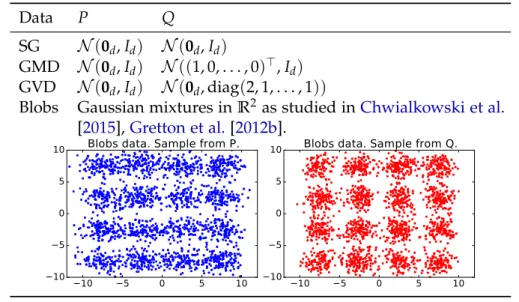
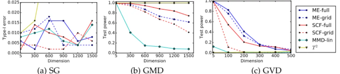
Summary We study two semimetrics on probability distributions [Chwialkowski et al., 2015], given as the sum of differences of expectations of analytic functions evaluated at spatial or frequency locations (i.e., features). The goal is to learn informative features for distinguishing two distributions. The features are learned so as to maximize the distinguishability of the distributions, by optimizing a lower bound on test power for a statistical test using these features. The result is a parsimonious and interpretable indication of how and where two distributions differ locally. We show that the empirical estimate of the test power criterion converges with increasing sample size, ensuring the quality of the returned features. In real-world benchmarks on high-dimensional text and image data, linear-time tests using the proposed semimetrics achieve comparable performance to the state-of-the-art quadratic-time maximum mean discrepancy test, while returning human-interpretable features that explain the test results.
3.1
Introduction
We address the problem of discovering features of distinct probability distributions, with which they can most easily be distinguished. The distributions may be in high dimensions, can differ in non-trivial ways (i.e., not simply in their means), and are observed only through i.i.d. samples. One application for such divergence measures is to model criticism, where samples from a trained model are compared with a validation sample: in the univariate case, through the KL divergence [Cinzia Carota and Polson,1996], or in the multivariate case, by use of the maximum mean discrep-ancy (MMD) [Lloyd and Ghahramani, 2015] (see Section2.3for an introduction to MMD). In the latter work, the model output of the Automated Statistician [Lloyd et al., 2014] is compared with the original sample via a smooth witness function, which has largest amplitude where the sample probability mass differs most from the model. An alternative, interpretable analysis of a multivariate difference in distributions may be obtained by projecting onto a discriminative direction, such that the Wasserstein
distance on this projection is maximized [Mueller and Jaakkola,2015]. Note that both recent works require low dimensionality, either explicitly (in the case of Lloyd and Gharamani, the function becomes difficult to plot in more than two dimensions), or implicitly in the case of Mueller and Jaakkola, in that a large difference in distributions must occur in projection along a particular one-dimensional axis. Distances between distributions in high dimensions may be more subtle, however, and it is of interest to find interpretable, distinguishing features of these distributions. For example, when divergence measures are used in adversarial learning for deep belief networks [Dziugaite et al.,2015,Li et al.,2015], it might be of interest to reveal explicitly the manner in which the distributions returned by samples from the model differ from the validation sample, which is challenging given the high dimensional outputs of the models.
In this chapter, we take a hypothesis testing approach to discovering features which best distinguish two multivariate probability measuresPandQ, as observed by samples X := {xi}ni=1 drawn independently and identically (i.i.d.) from P, and
Y := {yi}ni=1 ⊂ X ⊆Rd from Q. Non-parametric two-sample tests based on RKHS
distances [Moulines et al.,2008,Fromont et al.,2012,Gretton et al.,2012a] or energy distances [Székely and Rizzo, 2004, Baringhaus and Franz, 2004] have as their test statistic an integral probability metric, the Maximum Mean Discrepancy [Gretton et al., 2012a, Sejdinovic et al., 2013]. For this metric, a smooth witness function is computed, such that the amplitude is largest where the probability mass differs most [e.g.Gretton et al.,2012a, Figure 1].Lloyd and Ghahramani[2015] used this witness function to compare the model output of the Automated Statistician [Lloyd et al., 2014] with a reference sample, yielding a visual indication of where the model fails. In high dimensions, however, the witness function cannot be plotted, and is less helpful. Furthermore, the witness function does not give an easily interpretable result for distributions with local differences in their characteristic functions. A more subtle shortcoming is that it does not provide a direct indication of the distribution features which, when compared, would maximize test power. Rather, it is the witness function norm, and (broadly speaking) itsvarianceunder the null, that determine test power.
Contributions Our approach builds on the analytic representations of probability distributions of Chwialkowski et al. [2015], where differences in expectations of analytic functions at particular spatial or frequency locations are used to construct a two-sample test statistic, which can be computed in linear time. Chwialkowski et al. [2015] showed that, despite the differences in these analytic functions being evaluated at random locations, the analytic tests have greater power than linear time tests based on subsampled estimates (see (2.14)) of the MMD [Gretton et al.,2012b,Zaremba et al., 2013]. Our first theoretical contribution, in Section3.4.1, is to derive a lower bound on the test power, which can be maximized over the choice of test locations (features). We propose two novel variants, both of which significantly outperform the random feature choice ofChwialkowski et al.. The Mean Embedding (ME) test evaluates the
difference of mean embeddings at locations chosen to maximize the test power lower bound (i.e., spatial features); unlike the maxima of the MMD witness function, these features are directly chosen to maximize the distinguishability of the distributions, and take variance into account. The Smooth Characteristic Function (SCF) test uses as its statistic the difference of the two smoothed empirical characteristic functions, evaluated at points in the frequency domain so as to maximize the same criterion (i.e., frequency features). Optimization of the mean embedding kernels/frequency smoothing functions themselves is achieved on a held-out data set with the same consistent objective.
As our second theoretical contribution in Section3.4.2, we prove that the empirical estimate of the test power criterion asymptotically converges to its population quantity uniformly over the class of Gaussian kernels, at the rate of Op(n−1/4), wheren is
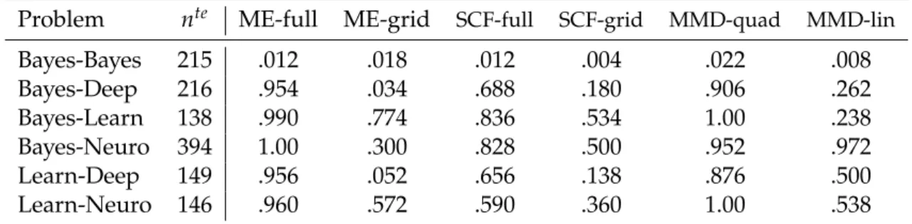
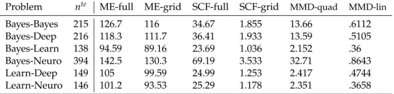
the sample size. Two important consequences follow: first, in testing, we obtain a more powerful test with fewer features. Second, we obtain a parsimonious and interpretable set of features that best distinguish the probability distributions. In Section3.5, we provide experiments demonstrating that the proposed linear-time tests greatly outperform all considered linear time tests, and achieve performance that compares to or exceeds the more expensive quadratic-time MMD test [Gretton et al., 2012a]. Moreover, the new tests discover features of text data (NIPS proceedings) and image data (distinct facial expressions) which have a clear human interpretation, thus validating our feature elicitation procedure in these challenging high-dimensional testing scenarios.
3.2
Mean Embedding (ME) Test
Our approach of discovering distinguishing features is formulated as a nonparametric two-sample test based on the mean embedding (ME) and the smooth characteristic function (SCF) tests [Chwialkowski et al., 2015]. In this section, we review the ME test. The SCF test will be described in Section 3.3. Given two i.i.d. samples X := {xi}ni=1,Y := {yi}ni=1 from P and Q on X ⊆ Rd, respectively, the goal of a
two-sample test is to decide whetherPis different from Qon the basis of the samples. The task is formulated as a statistical hypothesis test proposing a null hypothesis H0 : P = Q (samples are drawn from the same distribution) against an alternative
hypothesis H1 : P 6= Q (the sample generating distributions are different). A test
calculates a test statistic ˆλnfromXandY, and rejectsH0if ˆλnexceeds a predetermined
test threshold (critical value). The thresholdTα is given by the(1−α)-quantile of the distribution of ˆλnunder H0 i.e., the null distribution, andαis the significance level of
the test.
3.2.1 Unnormalized ME Statistic
The (unnormalized) ME test, in its simplest form, relies on a (random) metric on the space of Borel probability measures. Given a bounded, characteristic, integrable and real analytic kernel k: X × X → R (see Section 2.5: Properties of Kernels),
consider the mean embeddings of P and Qgiven respectively by µP := Ex∼Pk(x,·)
andµQ :=Ey∼Qk(y,·). The population unnormalized ME (UME) statistic is defined
such that its square is
UME2(P,Q) = 1 J J
∑
j=1 µP(vj)−µQ(vj) 2 , (3.1)whereV := {v1, . . . ,vJ}is the set oftest locationsat which the witness function (i.e.,
difference of the two mean embeddings. See (2.9)) is evaluated. Chwialkowski et al. [2015, Theorem 2] shows that ifV is drawn from a distribution with a density, then (3.1) is arandom metricon the space of Borel probability measures. A random metric [Chwialkowski et al.,2015, Definition 1] simply means that it is a metric in the usual sense with qualification “almost-surely” attached to each property of the metric. More precisely, ifV is drawn from a distributionηwhich has a density and whose support
is a subset ofX, thenη-almost surely UME(P,Q)is a metric. In particular,η-almost
surely UME(P,Q) =0 if and only ifP= Q. Theη-almost-sureness means that there
exists at least one setting of V such that UME(P,Q) = 0 does not imply P = Q. However, ifV ∼η, then such an “unlucky” event will not happen (more precisely, the
probability of such event is 0).
A consistent estimator of (3.1) is given by
\ UME2 = 1 J J
∑
j=1 ˆ µP(vj)−µˆQ(vj) 2 = 1 J J∑
j=1 zn,j 2 = 1 Jz > nzn, (3.2)where ˆµP(v) := n1∑ni=1k(xi,v)and ˆµQ(v) := 1n∑in=1k(yi,v)are empirical mean
em-beddings of PandQ, respectively,zn:= n1∑ni=1zi ∈RJ and
zi := [k(xi,v1)−k(yi,v1), . . . ,k(xi,vJ)−k(yi,vJ)]∈RJ.
If we assume that evaluation ofk(x,v)costsO(d), then clearly (3.2) can be computed inO(dJn)time, which is linear in the sample size. We note that the pairing ofxi andyi
inzi does not suggest any joint dependency betweenxi andyi. Any arbitrary pairing
yields an equivalent estimator. In principle,UME\2can be used as a test statistic for the
two-sample test. However, under H0, asn→∞,√nUME\2converges to a finite sum of
weighted chi-squared variables that are dependent.1 This distribution does not have a closed-form expression. Thus, determining(1−α)-quantile for the test threshold has
to rely on simulations from the asymptotic null distribution, or a permutation test, both of which can be costly.
1UnderH
0, for a fixedV, by the central limit theorem,√nzn,j→ Nd (0,V[k(x,vj)−k(x,vj)])for all j∈ {1, . . . ,J}. Thus,nz2n,j→d V[k(x,vj)−k(x,vj)]χ2(1)for allj∈ {1, . . .J}. The variablesnz2n,1, . . . ,nz2n,J
3.2.2 Normalized ME (NME) Statistic
Intractability of the asymptotic null distribution was the motivation to consider the normalized ME statistic [Chwialkowski et al.,2015, Eq. 13]. The empirical normalized ME statistic (NME) is defined as
\
NME2(P,Q) =λnˆ :=nz>
nS−n1zn, (3.3)
whereSn := n1∑in=1(zi−zn)(zi−zn)>∈RJ×Jandznis as in (3.2). The NME is a form
of Hotelling’s T-squared statistic [Anderson,2003, Chapter 5]. The presence of the inverse covariance matrixS−n1is to decorrelatezn,1, . . . ,zn,J, so that the asymptotic null
distribution is tractable. Asymptotic behaviors of ˆλn are summarized in Proposition 3.1.
Proposition 3.1(Asymptotic behaviors of ˆλn[Chwialkowski et al.,2015, Proposition
2]). SupposeUME2(P,Q) =0. Then, for fixed d, as n→∞,λˆn →d χ2(J), the chi-squared
random variable with J degrees of freedom. If UME2(P,Q) > 0, then for any fixed r,
P(λˆn>r)→1as n →∞.
Proposition3.1states that the asymptotic null distribution of ˆλnisχ2(J)which is
very simple. This asymptotic null distribution holds true regardless ofPandQ. This implies that whennis sufficiently large, one can simply compute the(1−α)-quantile
of χ2(J) for the test threshold. Under H1, the probability of correctly rejecting H0
approaches 1 asn→∞. These two facts mean that the NME test is consistent.
3.3
Smooth Characteristic Function (SCF) Test
The SCF test relies on the difference of smoothed (by a kernel) characteristic functions of Pand QonX ⊆ Rd, evaluated at J frequencies. Let ϕP(t):= Ex∼P[eit
>x
] be the characteristic function of P where i = √−1. Similarly, ϕQ(t) := Ey∼P[eit
>y
]. To motivate the importance of the smoothing operation on the characteristic functions, consider the difference of (non-smoothed) characteristic functions [Epps and Singleton, 1986]: ρ2ϕ(P,Q):= 1 J J
∑
j=1 |ϕP(vj)−ϕQ(vj)|2, (3.4)whereV :={vj}jJ=1is the set of frequency values at which the characteristic function
difference is evaluated. The setV plays the same role (in the frequency domain) as the spatial test locations of the ME test. While (3.4) can be estimated efficiently inO(dJn)
time (assuming the use of empirical characteristic functions), it turns out thatρϕ(P,Q) is only a pseudometric. In particular,ρ2ϕ(P,Q) =0 does not always implyP= Q, as
summarized in Proposition3.2.
Proposition 3.2(Chwialkowski et al.[2015, Proposition 1]). Let J ∈Nand let{vj}jJ=1