________________
*Corresponding author
Received October 15, 2016
175
Available online at http://scik.org
J. Math. Comput. Sci. 7 (2017), No. 1, 175-188
ISSN: 1927-5307
ON A BATCH ARRIVAL QUEUE WITH SECOND OPTIONAL SERVICE,
RANDOM BREAKDOWNS, DELAY TIME FOR REPAIRS TO START AND
RESTRICTED AVAILABILITY OF ARRIVALS DURING BREAKDOWN
PERIODS
KAILASH C. MADAN* AND EBRAHIM MALALLA
Department of Mathematical Sciences, College of Arts, Science and Education, Ahlia University, Kingdom of Bahrain
Copyright © 2017 Madan and Malalla. This is an open access article distributed under the Creative Commons Attribution License, which permits unrestricted use, distribution, and reproduction in any medium, provided the original work is properly cited.
Abstract: We study a batch arrival single service channel queuing system where the server (service channel) provides two stages of general service to customers, the first essential service followed by the second optional service. It is assumed that the service channel is subject to breakdowns and on the occurrence of a breakdown, the service channel waits for the repairs to start and this waiting time (termed as the set-up time or delay time for repairs) is assumed general. Further, the repair times are also assumed general. We employ the supplementary variable technique using four supplementary variables, one each for the elapsed service time of the first essential service, the elapsed service time of the second optional service, the elapsed delay time and the elapsed repair time. In addition, we add an important assumption that during breakdown periods, the arriving batches are admitted into the system based on a policy of restricted admissibility. We derive queue size distribution for this system at a random epoch under the steady state conditions. Further, we derive some important performance measures of this system. This extends many models studied earlier by several authors. Finally, a few interesting particular cases are discussed.
Keywords: first essential service; second optional service; random breakdowns; delay time; repair time; restricted admissibility; queue size distribution at a random epoch; steady state.
2010 AMS Subject Classification: 60K25.
1 Introduction
Server breakdowns are common in many queueing situations. During the repair times of the
Consequently, such breakdowns have a definite effect on the system, particularly on the queue
length and customers’ waiting time in the system. Among some earlier papers on service
interruptions, we refer the reader to [1], [3] and [6]. Recently, [5] and [12] have studied some
queueing systems with service interruptions and the present author [11] has studied a queueing
system with time-homogeneous server breakdowns and deterministic repair time. Most of these
and other systems assume single (one by one) arrivals and they further assume that as soon as the
service channel fails, the repairs start instantly. However, in the present paper, we deal with a
bulk input queue M /
G1 G2(Optional)
/1X
with random breakdowns and delayed repairs, in
which we assume that the service channel has to wait for the repairs to start, which is a much
more realistic assumption in many real-life queueing situations. This delay in starting repairs
may occur due to the non-availability of the repair people or the necessary apparatus needed for
the repairs. This type of delay time was earlier introduced by one of the present authors, [7] in an
M/M/1 queue with random breakdowns, general delay time and exponential repair time.
Recently, [2] studied a queueing system with random breakdowns and delay times. However, in
the present paper we attempt a wider generalization of the models studied by[7] and [2]. Not
only that, we also generalize [8] in which he introduced the idea of second optional service but
assumed single arrivals and assumed the second optional service times to be exponential. In this
paper, we assume that system receives input of customers in batches of variable size and that the
arriving customers are provided the first essential service (FES) followed by the second optional
service (SOS). However, we assume that the service times of FES, the service times of the SOS,
the delay time for the repairs to start and the repair time of the service facility, all the four
random variables, follow a general arbitrary distribution. We employ the supplementary variable
technique by introducing four independent supplementary variables, one each for these four
variables. We further assume that service facility may only fail while it is working unlike Madan
[10] who assumed that it may fail even when it is idle.
Another very important assumption in this work is the policy of restricted admissibility of
arriving groups during breakdown periods. [9] Introduced restricted admissibility of arrivals in a
vacation queue. In that paper, they assume that not all arriving batches are allowed to join the
system as a policy to control overflow of the input into the system. Subsequently, [10] studied a
vacation queue with restricted admissibility and assumed different restricted policies for the case
studied a queueing system with control policies different from the ones studied by [9] and [10].
In the present paper, unlike [9] and [10], we employ the policy of restricted admissibility of
batches only during the breakdown periods of the server. This is indeed a very valid and a
realistic assumption, which would help alleviate the system’s overall congestion.
2 Description of the Model and Definitions
We consider a batch arrival queueing system, where arrivals occur according to a compound
Poisson process with the batch size random variable ‘I’. The server provides FES, one by one, to
all customers on a first come, first served basis. On completion of the FES, a customer opts for
the SOS with probability p and leaves the system with probability1p. The two service time random variables S1 and S2of a customer follow a general probability law with respective distribution functions (DF) G1(x) and G2(x), Laplace-Stieltjes Transforms (LST) G1*() and
) ( * 2
G and finite moments
E
(
S
1k)
andE
(
S
2k)
,k
1
, respectively. It is further assumed that the server is subject to random breakdowns such that dt is the first order probability that the service channel will fail during the short interval of time (t,tdt]. We assume that as a result of a random breakdown, the unit whose service (FES or SOS) gets interrupted, instantlygoes back to the head of the queue. As soon as the server breaks down, it has to wait for the
repairs to start. We define this waiting time as the delay time and assume that the delay time random variable D follows a general probability law with DF D(x), LST D*() and finite moments E(DK), k 1. Next, we assume that the repair time random variable R of the service channel also follows a general probability law with DF R(x), LST R*() and finite moments
) (RK
E , k 1. Let c (0 c1) be the probability that an arriving batch will be allowed to join the system during the period of time when the server is under breakdown state, either waiting for
repairs to start or under repairs.
Next, we define batch arrival rate,X batch size (a random variable),
k
a Prob [Xk],
1 ) (
k k k
a z z
X , the PGF of X, and E[X[k]]E[X(X1)...(Xk1)], the k
-th factorial moment of X.
Further, since G1(x) , )G2(x , D(x) and R(x) are continuous at x=0, therefore,
) ( 1
) ( )
(
1 1 1
x G
x dG dx x
,
) ( 1
) ( )
(
2 2 2
x G
x dG dx x
) ( 1
) ( )
(
x D
x dD dx x
and
) ( 1
) ( )
(
x R
x dR dx x
are the
first order differential functions (hazard rates) of G1(x), G2(x), D(x) and R(x), respectively. Next, we define
) ; ( ) 1 (
t x
Wn = probability that at time t, there are n (1) customers in the system, including one customer being provided FES since the elapsed service time x,
) ; ( ) 2 (
t x
Wn = probability that at time t, there are n (1)customers in the system, including one customer being provided SOS since the elapsed service time x,
) ; (x t
FnD = probability that at time t, there are n (1) customers in the queue, the server is in the failed state and waiting for repairs to start with elapsed waiting time x,
) ; (xt FR
n = probability that at time t, there are n (1) customers in the queue and the server is under repairs with elapsed repair time x,
) (t
Q = probability that at time t, the system is empty and server is idle (but available in the system for service).
Now we shall analyze the limiting behavior of this queueing process at a random epoch with the
help of Kolmogorov forward equations provided the following limits exist and are independent
of the initial state:
t
Q
lim
Q(t),
t n
x
dx
W
(1)(
)
lim
,
)
,
(
) 1 (dx
t
x
W
n
t n
x
dx
W
(2)(
)
lim
W
n(2)(
x
,
t
)
dx
,
t D
n
x
dx
F
(
)
lim
F
nD(
x
,
t
)
dx
,
and
t R
n
x
dx
F
(
)
lim
F
nR(
x
,
t
)
dx
,
where x0, and n1.3 Steady State Equations Governing the System
Then following the usual probability reasoning, we have, for x0, and n1, the following set of Kolmogorov forward equations under the steady state conditions:
nk
k n k n
n
x
x
W
x
a
W
x
W
dx
d
1 ) 1 ( )
1 ( 1
) 1 (
),
(
)
(
)
(
)
(
(1)
nk
k n k n
n
x
x
W
x
a
W
x
W
dx
d
1
) 2 ( )
2 ( 2
) 2 (
),
(
)
(
)
(
)
n k D k n k D n D n Dn
x
x
F
x
c
F
x
c
a
F
x
F
dx
d
1),
(
)
(
)
1
(
)
(
)
(
)
(
(3)
n k R k n k R n R n Rn
x
x
F
x
c
F
x
c
a
F
x
F
dx
d
1),
(
)
(
)
1
(
)
(
)
(
)
(
(4)
0 0 2 ) 2 ( 1 1 ) 1 (1
(
)
(
)
(
)
)
1
(
p
W
x
x
dx
W
x
dx
Q
. (5)The above set of equations is to be solved under the following boundary conditions at
x = 0 and for n1:
0 0 2 ) 2 ( 1 0 1 ) 1 ( 1 ) 1 (,
)
(
)
(
)
(
)
(
)
(
)
(
)
1
(
)
0
(
a
Q
p
W
x
x
dx
W
x
x
dx
F
x
x
dx
W
Rn n
n n
n
(6)
0 1 ) 1 ( ) 2 ()
(
)
(
)
0
(
p
W
x
x
dx
W
n n
, (7)
(1) (2)
)
0
(
n nD
n
W
W
F
, where
0 ) ( ) ( 2 , 1 , ) (x dx j W
W j
n j
n , (8)
0)
(
)
(
)
0
(
F
x
x
dx
F
Dn R
n
, (9)and the normalizing condition
1
)
(
)
(
)
(
1 0 1 0
1 0 ) ( 2 1
n n
R n D n n j n j
dx
x
F
dx
x
F
dx
x
W
Q
. (10)4 Queue Size Distribution at a Random Epoch
Next, we define the following Probability Generating Functions for |z|1:
0
),
(
)
,
(
1 ) 1 ( ) 1 (
x
x
W
z
z
x
W
n n n ;
1 ) 1 ( ) 1 (),
0
(
)
,
0
(
n n nW
z
z
W
1 ) 1 ( 0 ) 1 ( ) 1 ()
,
(
)
(
n n nW
z
dx
z
x
W
z
W
, (11a)0
),
(
)
,
(
1 ) 2 ( ) 2 (
x
x
W
z
z
x
W
n n n ;
1 ) 2 ( ) 2 ()
0
(
)
,
0
(
n n nW
z
z
W
,
1 ) 2 ( 0 ) 2 ( ) 2 ()
,
(
)
(
n n nW
z
dx
z
x
W
z
0
),
(
)
,
(
1
x
x
F
z
z
x
F
n D n n D ;
1)
0
(
)
,
0
(
n D n n DF
z
z
F
,
0)
,
(
)
(
z
F
x
z
dx
F
D D, (11c)
0
),
(
)
,
(
1
x
x
F
z
z
x
F
n R n n R ;
1)
0
(
)
,
0
(
n R n n RF
z
z
F
,
0)
,
(
)
(
z
F
x
z
dx
F
R R. (11d)
We multiply equations (1) to (4) as well as the boundary conditions (6) to (9) by suitable
powers of z, sum over all possible values of n, use (5) and use (11). Thus we obtain the following results:
)
(
)
(
)
(
)
(
)
(
)
(
)
1
(
)
(
1
1
)
(
)
(
* * * 2 * 1 * 1 * 1 ) 1 (k
R
k
D
m
z
m
G
m
pG
m
G
p
z
Q
m
m
G
z
X
z
z
W
, (12)
)
(
)
(
)
(
)
(
)
(
)
(
)
1
(
)
(
1
)
(
1
)
(
)
(
* * * 2 * 1 * 1 * 2 * 1 ) 2 (k
R
k
D
m
z
m
G
m
pG
m
G
p
z
Q
m
m
G
m
G
z
X
z
p
z
W
, (13)
)
(
)
(
)
(
)
(
)
(
)
(
)
1
(
)
(
1
)
(
1
)
(
)
(
* * * 2 * 1 * 1 *k
R
k
D
m
z
m
G
m
pG
m
G
p
z
Q
k
k
D
m
z
X
z
z
F
D
, (14)
) ( ) ( ) ( ) ( ) ( ) ( ) 1 ( ) ( 1 ) ( ) ( 1 ) ( ) ( * * * 2 * 1 * 1 * * k R k D m z m G m pG m G p z Q k k R k D m z X z z F R
. (15)
Wherem
1X(z)
, k c
1X(z)
,
1 ( )
( )1 0 ) ( 1 *
1 X z e dG x
G
X z x
is the Laplace-Steiltjes transform of the firstessential service time,
1 ( )
2( )0
) ( 1 *
2 X z e dG x
G
X z x
transform of the second optional service time,
1
(
)
(
)
0
) ( 1 *
x
dD
e
z
X
c
D
c X z x
is theLaplace-Steiltjes transform of the waiting time before repairs to start, and
)
(
)
(
1
0
) ( 1 *
x
dR
e
z
X
c
R
c X z x
is the Laplace-Steiltjes transform of the repair time.Further, it is easy to see that at z=1 the right hand side expressions in equations (12) to (15) are
all of zero/zero form. Therefore, applying L’Hopital’s rule, we get
( ) ( ) ( ) ( )
) ( 1
) ( 1 ) ( )
( )
1 (
* 1 )
1 ( 1 )
1 (
R E D E X E X
E
Q G
X E z
W Lim W
z
, (16)
This is the steady state probability that at any random epoch, the server is busy providing first
essential service,
( ) ( ) ( ) ( )
) ( 1
) ( 1 ) ( ) ( )
( )
1 (
* 2 *
1 )
2 ( 1 )
2 (
R E D E X E X
E
Q G
G X E p z
W Lim W
z
, (17)
This is the steady state probability that at any random epoch, the server is busy providing second
optional service,
( ) ( ) ( ) ( )
) ( 1
) ( ) ( ) ( )
( )
1 (
1 E X E X E D E R
Q D
E X E z
F Lim
F D
z D
, (18)
This is the steady state probability that at any random epoch, the server is in the failed state and
waiting for repairs to start,
(
)
(
)
(
)
(
)
)
(
1
)
(
)
(
)
(
)
(
)
1
(
1
E
X
E
X
E
D
E
R
Q
R
E
X
E
z
F
Lim
F
Rz R
, (19)
This is the steady state probability that at any random epoch, the server is in the failed state and
under repairs.
Next, the normalizing condition in (10) is equivalent to
1 ) 1 ( ) 1 ( ) 1 ( )
1
( (2) )
1
(
D R
F F
W W
Q . (20)
) ( 1
) ( ) ( ) ( ) ( )
( 1
E X E X E D E R
Q . (21)
We note that (21) yields the following stability condition under which the steady state exists:
:
0
E(X ) E(X )
E(D) E(R)
() 1. (22)Finally, replacing the value of Q found in (21) in the numerators of equations (12) to (15), we
have explicitly determined all the probability generating functions. Similarly, equations (16) to
(19) can be simplified as follows.
) ( 1
) ( 1 ) ( )
( )
1 (
* 1 )
1 ( 1 )
1 (
G X
E z
W Lim W
z
, (23)
) ( 1
) ( 1 ) ( ) ( )
( )
1 (
* 2 *
1 )
2 ( 1 )
2 (
G G
X E p z W Lim W
z
, (24)
) ( 1
) ( ) ( ) ( )
( )
1 (
1
D E X E z
F Lim
F D
z D
, (25)
) ( 1
) ( ) ( ) ( )
( )
1 (
1
R E X E z
F Lim
F R
z R
, (26)
We may note that, the utilization factor of the system is the proportion of time the system is
busy providing the first essential service or the second optional service. Therefore, by adding
(4.6) and (4.7) and using the value of Q from (4.11), we obtain
)
(
1
)
(
)
(
E
X
. (27)Now, we define the probability generating function of the queue size distribution at a random
epoch irrespective of the state of the system as follows:
) ( ) ( ) ( )
( )
(z Q W(1) z W(2) z F z F z
P D R . (28)
This can be obtained by adding equations (12) to (15) and (21) and simplifying.
5 The Average System Size
|
1)
(
zz
P
dz
d
L
=
1 22 * 2 1 * 1 2 0 2 2
0
1
1
1
)
(
s se
s
E
G
p
e
s
E
G
X
E
+
1
2
(
)
(
)
2
)
(
2 20 2 2
R
E
D
E
R
E
D
E
X
E
+
0
0 1 ) ( 2 ) 1 (
X E X X E, (29)
where 0
E(X)E(X)
E(D)E(R)
() and E
X(X 1)
is the second factorial moment of batch size of arrivals.6 Some Particular Cases
Case 1: We assume single Poisson arrivals with no restricted admissibility and that FES, SOS,
Delay Time and Repair Time all have exponential distributions.
In this case we have, c=1,
E
(
X
)
1
,1 1 1 ) ( S E , 2 2 1 ) ( S E , 1 ) (D
E , ( 2) 22 D E , 1 ) (R
E , ( 2) 22
R
E ,
E
X
(
X
1
)
=0,
)) ( 1 ( ) ( 1 1 * 1 z X m G ,
1 1 *1
(
)
G
,
)) ( 1 ( ) ( 2 2 * 2 z X mG ,
2 2 *2( )
G , )) ( 1 ( ) ( * z X k D
, and
))
(
1
(
)
(
*z
X
k
R
.Consequently,
(1 ( )) 1 ) ( 1 1 * 1 z X m m G , 1 *
1( ) 1 1 G ,
(1 ( )) 1 ) ( 1 2 * 2 z X m m G , 2 *
2( ) 1 1 G , )) ( 1 ( 1 ) ( 1 * z X k k D
,
))
(
1
(
1
)
(
1
*z
X
k
k
R
, and ( ) ( 1 )( 2 )2 1
p .
With these substitutions in the main results we can obtain the corresponding to this case. In
) )( ( 1 1 ) 1 ( 2 1 2 1 1 ) 1 ( p
W , (30)
This is the steady state probability that at any random epoch the server is busy providing first
essential service, ) )( ( 1 1 ) 1 ( 2 1 2 1 2 1 1 ) 2 ( p p
W , (31)
This is the steady state probability that at any random epoch the server is busy providing second
optional service,
) )( ( 1 ) )( ( 1 ) 1 ( 2 1 2 1 2 1 2 1 p p
FD , (32)
This is the steady state probability that at any random epoch the server is in the failed state and
waiting for repairs to start,
) )( ( 1 ) )( ( 1 ) 1 ( 2 1 2 1 2 1 2 1 p p
FR , (33)
This is the steady state probability that at any random epoch the server is in the failed state and
under repairs.
Further, we have
) )( ( 1 ) )( ( 1 1 1 2 1 2 1 2 1 2 1 p p
Q , (34)
)
)(
(
1
)
)(
(
2 1 2 1 2 1 2 1
p
p
Further, since both service times are exponential, we have
1 *
1 ( )
1 G ,
2 *
2 ( )
1 G ,
21 1 1
)
(
1
se
s
E
and
22 2 2
)
(
2
se
s
E
.Therefore, (5.1) reduces to
L
2
2 2 1 0 2 0
) (
) (
1
1
p +
1
1
1
1
2 20 2
, (36)
where
)
)(
(
1
1
2 1
2 1
0
p
. (37)Case 2: No Second Optional Service
In this case, we put p0 in the main results. Case 3: No Delay
In this case, we haveD*
k 1 andE(D)0. Case 4: No BreakdownsIn this case, we let 0 and consequently, *
(
)
1
iG
, fori
1
,
2
, and) ( ) ( 1
1 *
1
0 E S
G
Lim
, ( )
) ( 1
2 *
2
0 E S
G
Lim
, ( ) ( 1) ( 2)
0 E S pE S
Lim
,
2
1
122 1 *
1 0
1
S
E
e
S
E
G
Lim
s
,
and
2
1
222 2 *
2 0
2
S
E
e
S
E
G
Lim
s
.
With these substitutions in the main results we can derive results of this particular case.
Case 5: No Second Optional Service, No Breakdowns
In this case we put p0 and E(S2)0 in the results of case 4 or we put 0 in the results of
case 2.
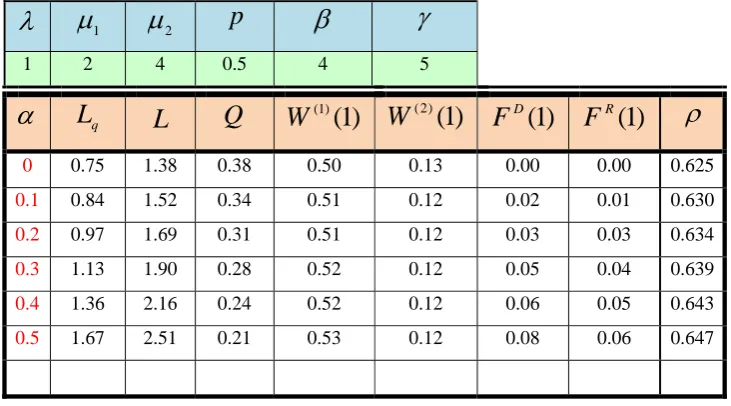
7 Numerical Examples
We provide some numerical examples to check the validity of our results obtained in Case 1 and
to see the effect of various parameters involved in our model (namely, the breakdown rate , the
the probabilities of various steady states of the system, namely the probabilities of the idle state,
the working state and the breakdown state waiting for repair to start and under repair. We assume
the fixed values of the arrival rate 1, the service rates
1
2
and
2
4
, and arbitrarily choose values of the other various parameters such that the stability condition (6.8) of theparticular case 1 is not violated. We obtain the following numerical values which depict results
as expected.
Table 1: Effect of
on the utilization factor and on the probabilities of steady states.
1
2p
1 2 4 0.5 0.5 5 0.647
L
qL
Q
(
1
)
) 1 (
W
(2)(
1
)
W
D(
1
)
F
R(
1
)
F
6 1.33 2.15 0.23 0.53 0.12 0.05 0.06
8 1.20 2.01 0.25 0.53 0.12 0.04 0.06
10 1.14 1.94 0.26 0.53 0.12 0.03 0.06
12 1.10 1.90 0.26 0.53 0.12 0.03 0.06
14 1.07 1.87 0.27 0.53 0.12 0.02 0.06
16 1.05 1.85 0.27 0.53 0.12 0.02 0.06
Table 2: Effect of
on the utilization factor and on the probabilities of steady states.
1
2p
1 2 4 0.5 4 5
L
qL
Q
(
1
)
) 1 (
W
(2)(
1
)
W
D(
1
)
F
R(
1
)
F
0 0.75 1.38 0.38 0.50 0.13 0.00 0.00 0.625
0.1 0.84 1.52 0.34 0.51 0.12 0.02 0.01 0.630
0.2 0.97 1.69 0.31 0.51 0.12 0.03 0.03 0.634
0.3 1.13 1.90 0.28 0.52 0.12 0.05 0.04 0.639
0.4 1.36 2.16 0.24 0.52 0.12 0.06 0.05 0.643
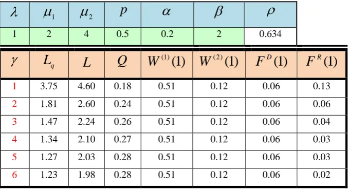
Table 3: Effect of
on the utilization factor and on the probabilities of steady states.
1
2p
1 2 4 0.5 0.2 2 0.634
L
qL
Q
(1)(
1
)
W
(2)(
1
)
W
D(
1
)
F
R(
1
)
F
1 3.75 4.60 0.18 0.51 0.12 0.06 0.13
2 1.81 2.60 0.24 0.51 0.12 0.06 0.06
3 1.47 2.24 0.26 0.51 0.12 0.06 0.04
4 1.34 2.10 0.27 0.51 0.12 0.06 0.03
5 1.27 2.03 0.28 0.51 0.12 0.06 0.03
6 1.23 1.98 0.28 0.51 0.12 0.06 0.02
Table 4: Effect of pon the utilization factor and on the probabilities of steady states.
1
2
1 2 4 0.5 6 4
p
L
qL
Q
(1)(
1
)
W
(2)(
1
)
W
D(
1
)
F
R(
1
)
F
0 0.71 1.40 0.40 0.50 0.00 0.04 0.06 0.500
0.2 0.92 1.67 0.33 0.51 0.05 0.05 0.07 0.557
0.4 1.26 2.06 0.26 0.52 0.09 0.05 0.08 0.616
0.6 1.90 2.77 0.18 0.54 0.14 0.06 0.08 0.679
0.8 3.60 4.53 0.10 0.55 0.20 0.06 0.09 0.744
1 21.24 22.23 0.02 0.56 0.25 0.07 0.10 0.813
One can easily notice that when increases for fixed values of and
, the probability of theidle state Q increases and the average queue length L decreases. Similarly, as
increases forfixed values of and . However, when increases for fixed values of and
, theprobability of the idle state Q decreases, the average queue length L increases and the utilization
factor
increases. Clearly, the utilization factor
increases as p increases for fixed values of, and
. On the other hand, it is independent of the delay parameter and the completion ofConflict of Interests
The authors declare that there is no conflict of interests.
REFERENCES
[1] B. Avi-Itzhak and P. Naor, Some Queueing Problems with the Service Station Subject to Breakdowns, Oper. Res., 11 (1963), 303-320.
[2] R. Fadhil, K. C. Madan and A. C. Lukas, On M(x)/G/1 Queueing System with Random Breakdowns, Server vacations, Delay Times and a Standby Server, International Journal of Operational Research, 15 (1) (2012), 30-47.
[3] D. P. Gaver, A Waiting Line with Interrupted Service Including Priorities, J. Roy. Statist. Soc., Ser. B, 24 (1962), 73-90.
[4] H. S. Lee and M. M. Srinivasan., Control Policies for the MX/G/1
Queueing Systems, Management Sciences, 35 (1989), 708-721.
[5] W. Li, D. Shi and X. Chao, Reliability Analysis of M/G/1 Queueing System with Server Breakdowns and Vacations, J. Appl. Prob., 34 (1997), 546-555.
[6] K. C. Madan, A Priority Queueing System with Service Interruption, Statistica Neerlandica, 27 (3) (1973), 115-123.
[7] K. C. Madan., A Queueing System with Random Failures and Delayed Repairs, Journal of Indian Stat. Ass., 32 (1994), 39-48.
[8] K. C. Madan, An M / G / 1 Queue with Second Optional Service, Queueing Systems, 34 (2000), 37-46.
[9] K. C. Madan and W. Abu-Dayyeh, Restricted Admissibility of Batches into an M/G/1 Type Bulk Queue with Modified Bernoulli Schedule Server Vacations, ESAIM: Probability and Statistics, 6 (2002), 113-125.
[10] K. C. Madan, and G. Choudhury, An M(X)/G/1 Queue with a Bernoulli Vacation Schedule Under Restricted Admissibility Policy, Sankhya, 66 (1) (2004), 175-193.
[11] K. C. Madan, An M / G / 1 Queue with Time-Homogeneous Breakdowns and Deterministic Repair Times, Soochow Journal of Mathematics, 29 (1) (2003), 103-110.