Adaptive estimator of the memory parameter and goodness-of-fit test using a multidimensional increment ratio statistic

Adaptive estimator of the memory parameter and

goodness-of-fit test using a multidimensional increment

ratio statistic

Jean-Marc Bardet, B´

echir Dola

To cite this version:

Jean-Marc Bardet, B´

echir Dola. Adaptive estimator of the memory parameter and

goodness-of-fit test using a multidimensional increment ratio statistic. Journal of Multivariate Analysis,

Elsevier, 2012, pp.222-240.

<

hal-00522842v2

>

HAL Id: hal-00522842

https://hal.archives-ouvertes.fr/hal-00522842v2

Submitted on 22 Sep 2011

HAL

is a multi-disciplinary open access

archive for the deposit and dissemination of

sci-entific research documents, whether they are

pub-lished or not.

The documents may come from

teaching and research institutions in France or

abroad, or from public or private research centers.

L’archive ouverte pluridisciplinaire

HAL

, est

destin´

ee au d´

epˆ

ot et `

a la diffusion de documents

scientifiques de niveau recherche, publi´

es ou non,

´

emanant des ´

etablissements d’enseignement et de

recherche fran¸

cais ou ´

etrangers, des laboratoires

publics ou priv´

es.

Adaptive estimator of the memory parameter and

goodness-of-fit test using a multidimensional increment

ratio statistic

Jean-Marc Bardet and B´echir Dola

[email protected] , [email protected]

SAMM, Universit´e Panth´eon-Sorbonne (Paris I), 90 rue de Tolbiac, 75013 Paris, FRANCE

September 22, 2011

Abstract

The increment ratio (IR) statistic was first defined and studied in Surgailiset al. _{(2007) for estimating}

the memory parameter either of a stationary or an increment stationary Gaussian process. Here three extensions are proposed in the case of stationary processes. Firstly, a multidimensional central limit theorem is established for a vector composed by several IR statistics. Secondly, a goodness-of-fitχ2-type test can be deduced from this theorem. Finally, this theorem allows to construct adaptive versions of the estimator and test which are studied in a general semiparametric frame. The adaptive estimator of the long-memory parameter is proved to follow an oracle property. Simulations attest of the interesting accuracies and robustness of the estimator and test, even in the non Gaussian case.

Keywords: Long-memory Gaussian processes; goodness-of-fit test; estimation of the memory parameter; minimax adaptive estimator.

1

Introduction

After almost thirty years of intensive and numerous studies, the long-memory processes form now an im-portant topic of the time series study (see for instance the book edited by Doukhanet al, 2003). The most famous long-memory stationary time series are the fractional Gaussian noises (fGn) with Hurst parameterH

and FARIMA(p, d, q) processes. For both these time series, the spectral densityf in 0 follows a power law:

f(λ)_∼C λ−2d _{where H =d+ 1/2 in the case of the fGn. In the case of long memory processd}

∈(0,1/2) but a natural expansion tod∈(−1/2,0] (short memory) implied thatdcan be considered more generally as a memory parameter.

There are a lot of statistical results relative to the estimation of this memory parameter d. First and main results in this direction have been obtained for parametric models with the essential articles of Fox and Taqqu (1986) and Dahlhaus (1989) for Gaussian time series, Giraitis and Surgailis (1990) for linear processes and Giraitis and Taqqu (1999) for non linear functions of Gaussian processes.

However parametric estimators are not really robust and can induce no consistent estimations. Thus, the research is now rather focused on semiparametric estimators of the memory parameter. Different approaches were considered: the famous R/S statistic (see Hurst, 1951), the log-periodogram estimator (studied firstly by Geweke and Porter-Hudack, 1983, notably improved by Robinson, 1995a, and Moulines and Soulier, 2003), the local Whittle estimator (see Robinson, 1995b) or the wavelet based estimator (see Veitch et al, 2003,

Moulineset al, 2007 or Bardetet al, 2008). All these estimators require the choice of an auxiliary parameter (frequency bandwidth, scales, etc.) but adaptive versions of these estimators are generally built for avoiding this choice. In a general semiparametric frame, Giraitis et al (1997) obtained the asymptotic lower bound for the minimax risk in the estimation of d, expressed as a function of the second order parameter of the spectral density expansion around 0. Several adaptive semiparametric estimators are proved to follow an oracle property up to multiplicative logarithm term. But simulations (see for instance Bardetet al, 2003 or 2008) show that the most accurate estimators are local Whittle, global log-periodogram and wavelet based estimators.

In this paper, we consider the IR (Increment Ratio) estimator of long-memory parameter (see its defini-tion in the next Secdefini-tion) for Gaussian time series recently introduced in Surgailiset al. (2007) and we propose three extensions. Firstly, a multivariate central limit theorem is established for a vector of IR statistics with different “windows” (see Section 2) and this induces to consider a pseudo-generalized least square estimator of the parameterd. Secondly, this multivariate result allows us to define an adaptive estimator of the memory parameterd based on IR statistics: an “optimal” window is automatically computed (see Section 3). This notably improves the results of Surgailiset al. (2007) in which the choice ofmis either theoretical (and cannot be applied to data) or guided by empirical rules without justifications. Thirdly, an adaptive goodness-of-fit test is deduced and its convergence to a chi-square distribution is established (see Section 3).

In Section 4, several Monte Carlo simulations are realized for optimizing the adaptive estimator and exhibiting the theoretical results. Then some numerical comparisons are made with the 3 semiparametric estimators previously mentioned (local Whittle, global log-periodogram and wavelet based estimators) and the results are even better than the theory seems to indicate: as well in terms of convergence rate than in terms of robustness (notably in case of trend or seasonal component), the adaptive IR estimator and goodness-of-fit test provide efficient results. Finally, all the proofs are grouped in Section 5.

2

The multidimensional increment ratio statistic and its statistical

applications

LetX = (Xk)k∈N be a Gaussian time series satisfying the following AssumptionS(d, β):

Assumption S(d, β): There exist ε > 0, c0 > 0, c′0 > 0 and c1 ∈ R such that X = (Xt)t∈Z is a

sta-tionary Gaussian time series having a spectral density f satisfying for all λ_∈(₋π,0)_∪(0, π)

f(λ) =c0|λ|−2d+c1|λ|−2d+β+O |λ|−2d+β+ε and |f′(λ)| ≤c′0λ−2d−1. (2.1)

Remark 1. Note that here we only consider the case of stationary processes. However, as it was already done in Surgailis et al. (2007), it could be possible, mutatis mutandis, to extend our results to the case of processes having stationary increments.

Let (X1,· · · , XN) be a path ofX. For m∈N∗, define the random variableIRN(m) such as

IRN(m) := 1 N₋3m N−_X3m−1 k=0 |(Pk+mt=k+1Xt+m−Pk+mt=k+1Xt) + (Pk+2mt=k+m+1Xt+m−Pk+2mt=k+m+1Xt)| |(Pk+m_t=k+1Xt+m−Pk+mt=k+1Xt)|+|(Pk+2mt=k+m+1Xt+m−Pk+2mt=k+m+1Xt)| .

From Surgailiset al. (2007), withmsuch thatN/m_{→ ∞}andm_{→ ∞},

r N m IRN(m)−EIRN(m) L −→ N→∞ N(0, σ 2_(d)),

where σ2(d) := 2 Z ∞ 0 Cov |Zd(0) +Zd(1)| |Zd(0)|+|Zd(1)| , |Zd(τ) +Zd(τ+ 1)| |Zd(τ)|+|Zd(τ+ 1)| dτ (2.2) and Zd(τ) := 1 p |4d+0.5_−4| Bd+0.5(τ+ 2)−2Bd+0.5(τ+ 1) +Bd+0.5(τ) (2.3)

withBH a standardized fractional Brownian motion (FBM) with Hurst parameterH∈(0,1).

Remark 2. This convergence was obtained for Gaussian processes in Surgailis et al. (2007), but there also exist results concerning a modified IR statistic applied to stable processes (see Vaiciulis, 2009) with a different kind of limit theorem. We may suspect that it is also possible to extend the previous central limit theorem to long memory linear processes (since a Donsker type theorem with FBM as limit was proved for long memory linear processes, see for instance Ho and Hsing, 1997) but such result requires to prove a non obvious central limit theorem for a functional of multidimensional linear process. Surgailis et al. (2007) also considered the case of i.i.d.r.v. in the domain of attraction of a stable law with index 0 < α <2 and skewness parameter

−1_≤β_≤1 and concluded thatIRN(m)converges to almost the same limit. Finally, in Bardet and Surgailis

(2011) a “continuous” version of the IR statistic is considered for several kind of continuous time processes (Gaussian processes, diffusions and L´evy processes).

Now, instead of this univariate IR statistic, define a multivariate IR statistic as follows: letmj =j m, j= 1,· · ·, p

with 2_≤p[N/m]₋4, and define the random vector (IRN(j m))1≤j≤p. Thus,pis the number of considered

window lengths of this multivariate statistic. In the sequel we naturally extend the results obtained for

m_∈N∗ _{tom∈(0,∞) by the convention: (IR}

N(j m))1≤j≤p = (IRN(j[m]))1≤j≤p (which change nothing to

the asymptotic results).

We can establish a multidimensional central limit theorem satisfied by (IRN(j m))1≤j≤p:

Property 2.1. Assume that AssumptionS(d, β)holds with −0.5< d <0.5andβ >0. Then

r N m IRN(j m)−EIRN(j m) 1≤j≤p L −→ [N/m]∧m→∞ N(0,Γp(d)) (2.4) withΓp(d) = (σi,j(d))1≤i,j≤p where for t∈R

σi,j(d) := Z ∞ −∞ Cov |Z (i) d (0) +Z (i) d (i)| |Z_d(i)(0)_|+_|Z_d(i)(i)_|, |Z_d(j)(τ) +Z_d(j)(τ+j)| |Z_d(j)(τ)_|+_|Z_d(j)(τ+j)_| dτ and Z_d(j)(τ) = p 1 |4d+0.5_−4| Bd+0.5(τ+ 2j)−2Bd+0.5(τ+j) +Bd+0.5(τ) . (2.5)

The proof of this property as well as all the other proofs are given in Appendix. Moreover we will assume in the sequel that Γp(d) is a definite positive matrix for alld∈(−0.5,0.5).

Remark 3. Note that Assumption S(d, β) are a little stronger than the conditions required in Surgailis et al. (2007) where f is supposed to satisfy f(λ) = c0|λ|−2d +O(|λ|−2d+β) and |f′(λ)| ≤ c′0λ−2d−1. Note

that Property 2.1 and following Theorem 1 and Proposition 1 are as well checked under these assumptions of Surgailis et al. (2007) even if β ≥2d+ 1 (case which is not consider in their Theorem 2.4). However our automatic procedure for choosing an adaptive scale m_eN requires to specify the second order of the expansion

of f and we prefer to already give results under such assumption. As in Surgailiset al. (2007), forr∈(−1,1), define the function Λ(r) by

Λ(r) := 2 π arctan r 1 +r 1₋r+ 1 π r 1 +r 1₋rlog( 2 1 +r). (2.6)

and ford_∈(₋0.5,1.5) let

Λ0(d) := Λ(ρ(d)) where ρ(d) := 4

d+1.5₋₉d+0.5₋₇

2(4₋4d+0.5₎ . (2.7)

The function d _∈ (₋0.5,1.5) _→ Λ0(d) is a C∞ increasing function. Now, Property 5.1 (see in Section

5) provides the asymptotic behavior of E[IR(m)] when m → ∞, which is E[IR(m)] ∼ Λ0(d) +Cm−β if

β < 2d+ 1, E[IR(m)] _∼ Λ0(d) +Cm−βlogm if β = 2d+ 1 and E[IR(m)] ∼ Λ0(d) +O(m−(2d+1)) if

β >2d+ 1 (C is a non vanishing real number depending on dandβ). Therefore by choosingmand N such as pN/mm−β

→0, pN/mm−β_logm

→0 and pN/mm−(2β+1)

→0 (respectively) whenm, N _{→ ∞}, the term E[IR(jm)] can be replaced by Λ0(d) in Property 2.1. Then, using the Delta-method with function

(xi)1≤i≤p7→(Λ0−1(xi))1≤i≤p, we obtain:

Theorem 1. Let dbN(j m) := Λ−01 IRN(j m) for 1 ≤j ≤p. Assume that Assumption S(d, β) holds with

−0.5< d <0.5 andβ >0. Then ifm∼C Nα with C >0 and(1 + 2β)−1∨(4d+ 3)−1< α <1 then

r N m b dN(j m)−d 1≤j≤p L −→ N→∞ N 0,(Λ′0(d))−2Γp(d) . (2.8)

Remark 4. Ifβ <2d+ 1, the estimatordbN(m)is a semiparametric estimator ofdand its asymptotic mean

square error can be minimized with an appropriate sequence(mN)reaching the well-known minimax rate of

convergence for memory parameter d in this semiparametric setting (see for instance Giraitis et al., 1997). Indeed, under AssumptionS(d, β)withd_∈(₋0.5,0.5)andβ >0and ifmN = [N1/(1+2β)], then the estimator

b

dN(mN) is rate optimal in the minimax sense,i.e.

lim sup N→∞ sup d∈(−0.5,0.5) sup f∈S(d,β) N1+22ββ ·E[(db N(mN)−d)2]<∞.

From the multidimensional CLT (2.8) a pseudo-generalized least square estimation (LSE) ofdis possible by defining the following matrix:

b

ΣN(m) := (Λ′0(dbN(m))−2Γp(dbN(m)). (2.9)

Since the function d _∈ (₋0.5,1.5) _7→ σ(d)/Λ′_{(d) is C}∞ _{it is obvious that under assumptions of Theorem 1} then b ΣN(m) −→P N→∞ (Λ ′ 0(d))−2Γp(d).

Then with the vectorJp:= (1)1≤j≤p and denotingJp′ its transpose, the pseudo-generalized LSE ofdis:

e dN(m) := Jp′ ΣbN(m)− 1 Jp− 1 Jp′ ΣbN(m)− 1 _b dN(mi)_1≤i≤p

It is well known (Gauss-Markov Theorem) that the Mean Square Error (MSE) ofdeN(m) is smaller or equal

than all the MSEs of dbN(jm),j = 1, . . . , p. Hence, we obtain under the assumptions of Theorem 2.8:

r N m deN(m)−d L −→ N→∞ N 0,Λ′0(d)−2 Jp′Γ−p1(d)Jp− 1 , (2.10) and Λ′ 0(d)−2 Jp′Γp−1(d)Jp− 1 ≤Λ′ 0(d)−2σ2(d).

Now, consider the following test problem: for (X1,· · ·, Xn) a path ofX a Gaussian time series, chose between

• H0: the spectral density ofX satisfies AssumptionS(d, β) with−0.5< d <0.5 andβ >0;

• H1: the spectral density ofX does not satisfy such a behavior.

We deduce from the multidimensional CLT (2.8) aχ2_{-type goodness-of-fit test statistic defined by:}

b TN(m) := N m deN(m)−dbN(j m) ′ 1≤j≤p ΣbN(m) −1 e dN(m)−dbN(j m)_1≤j≤p.

Proposition 1. Under the assumptions of Theorem 1 then: b TN(m) −→L N→∞ χ 2_(p −1).

3

Adaptive versions of the estimator and goodness-of-fit test

Theorem 1 and Proposition 1 are interesting but they require the knowledge ofβ to be used (and therefore an appropriated choice of m). We suggest now a procedure (see also Bardet et al., 2008) for obtaining a data-driven selection of an optimal sequence (mN). For d∈(−0.5,1.5) andα∈(0,1), define

QN(α, d) := dbN(j Nα)−d′_1≤j≤p ΣbN(Nα)− 1 _b

dN(j Nα)−d_1≤j≤p. (3.1)

Note that by the previous convention, dbN(j Nα) = dbN(j[Nα]) and deN(Nα) = deN([Nα]). Thus QN(α, d)

corresponds to the sum of the pseudo-generalized squared distance. From previous computations, it is obvious that for a fixedα∈(0,1),Qis minimized bydeN(Nα) and therefore for 0< α <1 define

b

QN(α) :=QN(α,deN(Nα)).

It remains to minimizeQbN(α) on (0,1). However, sinceαbN has to be obtained from numerical computations,

the interval (0,1) can be discretized as follows,

b αN ∈ AN = n ₂ logN , 3 logN , . . . , log[N/p] logN o .

Hence, ifα_{∈ A}N, it exists k∈ {2,3, . . . ,log[N/p]}such thatk=αlogN. Consequently, define αbN by

b

QN(αbN) := min α∈AN

b

QN(α).

From the central limit theorem (2.8) one deduces the following :

Proposition 2. Assume that Assumption S(d, β) holds with −0.5 < d < 0.5 and β > 0. Moreover, if

β >2d+ 1, suppose thatc0, c1, c2, d, β andεare such that Condition (5.13) or (5.14) holds. Then,

b

αN −→P N→∞ α

∗₌ 1

(1 + 2β)_∧(4d+ 3).

Remark 5. The choice of the set of discretization _AN is implied by our proof of convergence ofαbN toα∗. If

the interval (0,1)is stepped in Nc _{points, withc >0, the used proof cannot attest this convergence. However}

logN may be replaced in the previous expression of_AN by any negligible function ofN compared to functions

Nc _{with c >0 (for instance,(logN)}a _{or alogN can be used).}

Remark 6. The reference to Condition (5.13) or (5.14) is necessary because our proof of the convergence of α_bN to α∗ requires to know the exact convergence rate of E[IRN(Nα)]−Λ0(d) when α < α∗. When

β ≤ 2d+ 1, since we replaced the conditions on the spectral density of Surgailis et al. (2007) by a second order condition (Assumption S(d, β)), this convergence rate can be obtained by computations (see Property 5.1). But if β >2d+ 1, we can only obtain E[IRN(Nα)]−Λ0(d) = O(m−2d−1) under AssumptionS(d, β):

the convergence rate could be slower than m−2d−1 _{and then}

b

αN could converge to α′ < α∗ (from the proof of

Proposition 2). Condition (5.13) and (5.14), which are not very strong, allow to obtain a first order bound for E[IRN(Nα)]−Λ0(d) (see Proposition 5.2) and hence to proveαbN −→P

N→∞ α ∗_.

From a straightforward application of the proof of Proposition 2, the asymptotic behavior of _baN can be

specified, that is,

Pr N α∗ (logN)λ ≤N b αN ≤Nα∗ ·(logN)µ −→ N→∞ 1, (3.2)

for all positive real numbers λ and µ such that λ > 2α∗

(p−2)(1−α∗₎ and µ >

12

p−2. Consequently, the selected

windowm_bN =NbαN asymptotically growths asNα

∗

up to a logarithm factor.

Finally, Proposition 2 can be used to define an adaptive estimator of d. First, define the straightfor-ward estimator deN(NαbN), which should minimize the mean square error using αbN. However, the

estima-tor deN(NαbN) does not satisfy a CLT since Pr(αbN ≤ α∗) > 0 and therefore it can not be asserted that

E(pN/NαbN_(de

N(NαbN)−d)) = 0. To establish a CLT satisfied by an adaptive estimator ofd, a (few) shifted

sequence of α_bN, so called αeN, has to be considered to ensure Pr(αeN ≤ α∗) −→

N→∞ 0. Hence, consider the adaptive scale sequence (meN) such as

e mN :=NαeN with αeN :=αbN + 6_bαN (p₋2)(1₋α_bN)· log logN logN .

and the estimator

e

d(IR)N :=deN(meN) =deN(NαeN).

The following theorem provides the asymptotic behavior of the estimatorde(IR)_N :

Theorem 2. Under assumptions of Proposition 2,

r N NαeN de (IR) N −d L −→ N→∞ N 0 ; Λ′0(d)−2 Jp′Γ−p1(d)Jp− 1 . (3.3) Moreover, if β≤2d+ 1, ∀ρ >2(1 + 3β) (p−2)β , N1+2ββ (logN)ρ · ed(IR)N −d P −→ N→∞ 0.

Remark 7. When β _≤2d+ 1, the adaptive estimator de(IR)_N converges to d with a rate of convergence rate equal to the minimax rate of convergenceN1+2ββ _{up to a logarithm factor (this result being classical within this}

semiparametric framework). Thus there exists ℓ <0 such that

N1+22ββ_(logN)ℓ_E(de(IR)

N −d) 2_<

∞.

Therefore de(IR)_N satisfies an oracle property for the considered semiparametric model.

If β >2d+ 1, the estimator is not rate optimal. However, simulations (see the following Section) will show that even if β > 2d+ 1, the rate of convergence of de(IR)_N can be better than the one of the best known rate optimal estimators (local Whittle or global log-periodogram estimators).

Moreover an adaptive version of the previous goodness-of-fit test can be derived. Thus define

e

T_N(IR):=TbN(NαeN). (3.4)

Then,

Proposition 3. Under assumptions of Proposition 2,

e

T_N(IR) _−→L

N→∞ χ

2_(p

−1).

4

Simulations and Monte-Carlo experiments

In the sequel, the numerical properties (consistency, robustness, choice of the parameter p) of de(IR)_N are investigated. Then the simulation results of de(IR)N are compared to those obtained with the best known

semiparametric long-memory estimators.

Remark 8. Note that all the softwares (in Matlab language) used in this Section are available with a free access on http://samm.univ-paris1.fr/-Jean-Marc-Bardet.

To begin with, the simulation conditions have to be specified. The results are obtained from 100 generated independent samples of each process belonging to the following ”benchmark”. The concrete procedures of generation of these processes are obtained from the circulant matrix method, as detailed in Doukhanet al. (2003). The simulations are realized for different values of d, N and processes which satisfy Assumption

S(d, β):

1. the fractional Gaussian noise (fGn) of parameterH=d+ 1/2 (for₋0.5< d <0.5) andσ2_{= 1. Such a}

process is such that AssumptionS(d,2) holds;

2. the FARIMA[p, d, q] process with parameter d such that d ∈ (−0.5,0.5), the innovation variance σ2

satisfyingσ2_{= 1 andp, q}

∈N_{. A FARIMA[p, d, q] process is such that Assumption S(d,2) holds;}

3. the Gaussian stationary process X(d,β)_{, such as its spectral density is}

f3(λ) =

1

λ2d(1 +λ

β_{) forλ}

∈[₋π,0)_∪(0, π], (4.1) withd_∈ (₋0.5,0.5) andβ _∈(0,_∞). Therefore the spectral density f3 is such as Assumption S(d, β)

holds.

A ”benchmark” which will be considered in the sequel consists of the following particular cases of these processes ford=₋0.4,₋0.2,0,0.2,0.4:

• fGn processes with parametersH =d+ 1/2;

• FARIMA[0, d,0] processes with standard Gaussian innovations;

• FARIMA[1, d,1] processes with standard Gaussian innovations and AR coefficientφ = −0.3 and MA coefficientφ= 0.7;

• X(d,β)_{Gaussian processes withβ= 1.}

4.1

Application of the IR estimator and tests applied to generated data

Choice of the parameter p: This parameter is important to estimate the ”beginning” of the linear part of the graph drawn by points (i, IR(im))i. On the one hand, ifpis a too small a number (for instancep= 3),

another small linear part of this graph (even before the ”true” beginningNα∗

) may be chosen. On the other hand, ifpis a too large a number (for instancep= 50 forN = 1000), the estimatorα_eN will certainly satisfy

e

αN < α∗ since it will not be possible to considerpdifferent windows larger thanNα

∗

. Moreover, it is possible that a ”good” choice ofpdepends on the ”flatness” of the spectral densityf, i.e. onβ. We have proceeded to simulations for several values ofp(and N and d). Only√M SE of estimators are presented. The results are specified in Table 1.

Conclusions from Table 1: it is clear that de(IR)_N converges todfor the four processes, the faster for fGn and FARIMA(0, d,0). The optimal choice ofpseems to depend onN for the four processes: _bp= 10 forN = 103_,

b

p= 15 forN= 104 _and

b

p_∈[15,20] forN = 105_{. The flatness of the spectral density of the process does not}

seem to have any influence, as well as the value of d(result obtained in the detailed simulations). We will adopt in the sequel the choicep_b= [1.5 log(N)] reflecting these results. At the contrary to the choice ofm, this choice ofponly depends onN and even if the adaptive scalem_eN depends onpits value does not change

a lot whenp_{∈ {}10,_{· · ·},20_}for 103

≤N _≤105_.

Concerning the adaptive choice ofm, the main point to be remarked is that the smoother the spectral density the smallerm; thusm_eN is smaller for a trajectory of a fGn or a FARIMA(0, d,0) than for a trajectory of a

FARIMA(1, d,1) orX(d,1)_{. The choice ofpdoes not appear to significantly affect the value of me}

N. More

and p= 15, the mean of m_eN is respectively equal to 23.9, 8.3, 4.5, 4.2 and 3.8 for d respectively equal to

−0.4, ₋0.2, 0, 0.2 and 0.4. This phenomena can be deduced from the theoretical study sinceα∗_{= (4d+ 3)}−1

in this case and thereforem_eN almost growths asN(4d+3)

−1

.

Finally, concerning the goodness-of-fit test, we remark that it is too conservative forp= 5 or 10 but close to the expected results forp= 15 and 20, especially for FARIMA(1, d,1) orX(d,1)_.

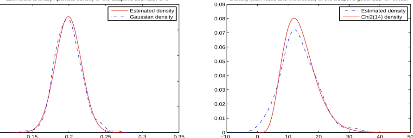
Asymptotic distributions of the estimator and test: Figure 1 provides the density estimations of

e

d(IR)_N and Te_N(IR)for 100 independent samples of FGN processes with d= 0.2 withN = 104 _{forp= 15. The}

goodness-of-fit to the theoretical asymptotic distributions (respectively Gaussian and chi-square) is satisfying.

0.1 0.15 0.2 0.25 0.3 0.35 0 5 10 15 20 25

Estimated and asymptotical density of the adaptive estimator of d Estimated density Gaussian density −100 0 10 20 30 40 50 0.01 0.02 0.03 0.04 0.05 0.06 0.07 0.08 0.09

Density (estimated and theoretical) of the adaptive goodness−of−fit test Estimated density Chi2(14) density

Figure 1: Density estimations and corresponding theoretical densities of de(IR)_N andTe_N(IR) for 100 samples of fGn withd= 0.2 withN = 104 andp= 15.

4.2

Comparison with other adaptive semiparametric estimator of the memory

parameter

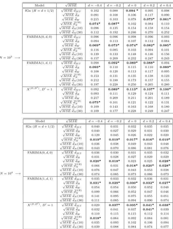
Consistency of semiparametric estimators: Here we consider the previous ”benchmark” and apply the estimatorde(IR)_N and 3 other semiparametric estimators ofdknown for their accuracies are considered:

• dbMS is the adaptive global log-periodogram estimator introduced by Moulines and Soulier (1998, 2003),

also called FEXP estimator, with bias-variance balance parameterκ= 2;

• dbRis the local Whittle estimator introduced by Robinson (1995). The trimming parameter ism=N/30;

• dbW is an adaptive wavelet based estimator introduced in Bardetet al. (2008) using a Lemarie-Meyer

type wavelet (another similar choice could be the adaptive wavelet estimator introduced in Veitchet al., 2003, using a Daubechie’s wavelet, but its robustness property are quite less interesting).

• de(IR)N defined previously withp= [1.5∗log(N)].

• dbN(10) and dbN(30) which are the (univariate) IR estimator with m = 10 and m = 30 respectively,

Simulation results are reported in Table 2.

Conclusions from Table 2: The adaptive IR estimatorde(IR)_N numerically shows a convincing convergence rate with respect to the other estimators.

The estimatorsdbN(10) anddbN(30) are clearly the worst estimators ofd. This can be explained by two facts:

1/ the numerical expression of the matrix ΣbN(m) is almost a diagonal matrix: therefore a least square

re-gression using several window lengths provides better estimations than an estimator using only one window length; 2/dbN(10) anddbN(30) use a fixed window length (m= 10 andm= 30) for any process andN while

we know thatm≃Nα∗

is the optimal choice which is approximated bymeN.

Both the “spectral” estimator dbR and dbMS provide more stable results that do not depend very much on

d and the process, while the wavelet based estimatordbW and de(IR)N are more sensible to the flatness of the

spectral density. But, especially for “smooth processes” (fGn and FARIMA(0, d,0)),de(IR)_N is a very accurate semiparametric estimator and is globally more efficient than the other estimators.

Robustness of the different semiparametric estimators: To conclude with the numerical properties of the estimators, five different processes not satisfying AssumptionS(d, β) are considered:

• a FARIMA(0, d,0) process with innovations satisfying a uniform law;

• a FARIMA(0, d,0) process with innovations satisfying a symmetric Burr distribution with cumulative distribution functionF(x) = 1−1

2 1

1+x2 forx≥0 andF(x) = 1_21+x12 forx≤0 (and therefore E|Xi|2=∞

but E_|Xi|<∞);

• a FARIMA(0, d,0) process with innovations satisfying a symmetric Burr distribution with cumulative distribution function F(x) = 1₋1

2 1

1+|x|3/2 for x≥ 0 and F(x) = 1_21+|x1_|3/2 for x≤ 0 (and therefore

E|Xi|2=∞but E|Xi|<∞);

• a Gaussian stationary process with a spectral density f(λ) = _||λ_{| −}π/2_|−2d _{for all λ}

∈ [₋π, π]_\

{−π/2, π/2}: this is a GARMA(0, d,0) process. The local behavior off in 0 isf(|λ|)∼(π/2)−2d_|λ|−2d

withd= 0, but the smoothness condition for f in AssumptionS(0, β) is not satisfied.

• a trended fGn with parameterH =d+ 0.5 and an additive linear trend;

• a fGn (H =d+ 0.5) with an additive linear trend and an additive sinusoidal seasonal component of periodT = 12.

The results of these simulations are given in Table 3.

Conclusions from Table 3: The main advantage of dbW and deN(IR) with respect to dbMS and dbR is

exhib-ited in this table: they are robust with respect to smooth trends, especially in the case of long memory processes (d >0). This has already been observed in Bruzaite and Vaiciulis (2008) for IR statistic (and even for certain discontinuous trends). Both those estimators are also robust with respect to seasonal component and this robustness would have been improved if we had chosen m (or scales) as a multiple of the period (which is generally known).

The second good surprise of these simulations is that the adaptive IR estimator de(IR)_N is also consistent for non Gaussian distributions even if the function Λ in (2.6) and therefore all our results are typically obtained for Gaussian distributions. The case of finite-variance processes is not surprising (see Remark 2). But this is more surprising for infinite variance processes. A first explanation of this was given in Surgailiset al. (2007) in the case of i.i.d.r.v. in the domain of attraction of a stable law with index 0< α <2 and skewness parameter

−1 _≤β _≤1: they concluded that IRN(m) converges to almost the same limit. The extension to α-stable

statistic (which is bounded in [0,1] for any processes) could allow to apply it to infinite variance processes. Note that the other semiparametric estimators are also consistent in such frame with faster convergence rates notably for the local Whittle estimator.

5

Proofs

Proof of Property 2.1. We proceed in two steps.

Step 1: First, we compute the limit of N_mCov IRN(jm), IRN(j′m) when N, m and N/m → ∞. As in

Surgailiset al(2007), define also for allj= 1,_{· · ·}, pand k= 1,_{· · ·}, N₋3mj (withmj=jm):

Ymj(k) := 1 Vmj k+m_Xj t=k+1 (Xt+mj−Xt) , with V 2 mj := E hk+m_Xj t=k+1 (Xt+mj −Xt) 2i (5.1) and ηmj(k) := |Ymj(k) +Ymj(k+mj)| |Ymj(k)|+|Ymj(k+mj)| . (5.2)

Note thatYmj(k)∼ N(0,1) for any kandj and

IRN(mj) = 1 N₋3mj N−3mj−1 X k=0 ηmj(k) for allj= 1,· · ·p. Cov(IRN(mj), IRN(mj′)) = 1 N₋3mj 1 N₋3mj′ N−3mj−1 X k=0 N−3mj′−1 X k′=0 Cov(ηmj(k), ηmj′(k ′₎₎₎ = 1 (_mN_{j −}3)(_mN j′ −3) Z N−1 mj −3 τ=0 Z N−1 m_j′ −3 τ′=0 Cov(ηmj([mjτ]), ηmj′([mj′τ′])))dτ dτ′. Now according to (5.20) of the same article, with−→F DD denoting the finite distribution convergence when

m_{→ ∞},

Ym([mτ]) −→F DD Zd(τ)

whereZdis defined in (2.3). Now

Yjm(k) = 1 Vmj jm X t=1 Xt+jm+1− jm X t=1 Xt+1Xt) = 1 Vmj j−1 X i=−(j−1) (j_{− |}i_|)VmYm(t+ (j+i−1)m). ButV2

m∼c0V(d)m2d+1whenm→ ∞(see (2.20) in Surgailiset al, 2007). Therefore we obtainYjm([mjτ])∼ 1

jd+1/2

Pj−1

i=−(j−1)(j− |i|)Ym([mjτ] + (j+i−1)m) whenm→ ∞(in distribution) and more generally,

Yjm([mjτ]), Yj′m([mj′τ′]) −→F DD ₁ jd+1/2 j−1 X i=−(j−1) (j− |i|)Zd(jτ+j+i−1), 1 (j′₎d+1/2 j′₋₁ X i′_=−(j′₋₁₎ (j′− |i′|)Zd(j′τ′+j′+i′−1) , (5.3)

whenm_{→ ∞}. Hence, obvious computations lead to define for t_∈R

Z_d(j)(t) := j−1 X i=−(j−1) (j_{− |}i_|)Zd(t+j+i−1) = Bd+0.5(t+ 2j)−p2Bd+0.5(t+j) +Bd+0.5(t) |4d+0.5_−4| (5.4) γ_d(j,j′)(t) := Cov ψ(Z_d(j)(0), Z_d(j)(j)), ψ(Z_d(j′)(t), Z_d(j′)(t+j′)). (5.5)

Now, as the function ψ(x, y) = _|x|x+y_|+|y|_| is a continuous (on R2

\ {0,0_}) and bounded function (with 0 _≤

ψ(x, y)_≤1) and sinceηmj([mjτ]) =ψ(Ymj([mjτ]), Ymj([mj(τ+ 1)])), then from (5.3),

Cov ηmj([mjτ]), ηmj′([mj′τ ′_{]) −→} m→∞ Cov ψ(Z (j) d (jτ), Z (j) d (j(τ+ 1))), ψ(Z (j′₎ d (j′τ′), Z (j′₎ d (j′(τ′+ 1))) −→ m→∞ γ (j,j′₎ d (j′τ′−jτ),

using the stationarity of the processZd and therefore of processesZd(j) and Z (j′₎

d . Hence, when N, m and

N/m→ ∞, N mCov(IRN(jm), IRN(j ′_{m)) ∼} N m(_jmN −3)(_jN′m−3) × Z N−1 jm −3 0 Z N−1 j′m−3 0 Cov ψ(Z_d(j)(j τ), Z_d(j)(j τ+j)), ψ(Z_d(j′)(j′_τ′_{), Z}(j′₎ d (j′τ′+j′)) dτ dτ′ ∼ _(N mN −3jm)(N₋3j′_m) Z N−1 m −3j 0 Z N−1 m −3j′ 0 γ(j,j_d ′)(s′₋s)ds ds′ ∼ m_N Z N m −N m N m − |u| γ_d(j,j′)(u)du −→ Z ∞ −∞ γ_d(j,j′)(u)du=:σj,j′(d). (5.6) This last limit is obtained, mutatis mutandis, from the relation (5.23) Surgailis et al (2007), and thus

γ_d(j,j′)(u) = C(u−2_{∧1), implying} m N RN m −N m | u|γ_d(j,j′)(u)du −→ N, m, N m→∞

0. It achieves the first step of the proof.

Step 2: It remains to prove the multidimensional central limit theorem. Then consider a linear combi-nation of (IRN(mj))1≤j≤p, i.e. Ppj=1ujIRN(mj) with (u1,· · · , up) ∈ Rp. For ease of notation, we will

restrict our purpose to p = 2, with mi = rim where r1 ≤ r2 are fixed positive integers. Then with the

previous notations and following the notations and results of Theorem 2.5 of Surgailiset al. (2007):

u1IRN(r1m) +u2IRN(r2m) =u1(E[IRN(r1m)] +SK(r1m) +SeK(r1m))

+u2(E[IRN(r2m)] +SK(r2m) +SeK(r2m)).

From (5.31) of Surgailis et al. (2007), we have SeK(m1) = o(SK(m1)) and SeK(m2) = o(SK(m2)) when

K _{→ ∞} and from an Hermitian decomposition (N/m)1/2_(u

1SK(mi) +u2SK(m2)) →D N(0, γK2) as N, m

and N/m → ∞ since the cumulants of (N/m)1/2_(u

1SK(mi) +u2SK(m2)) of order greater or equal to 3

converge to 0 (since this result is proved for each SK(mi)). Moreover, from the previous computations,

γ2

K→(u21σr1,r1(d) + 2u1u2σr1,r2(d) +u

2

2σr2,r2(d)) whenK→ ∞. Therefore the multidimensional central limit

theorem is established.

Property 5.1. Let X satisfy Assumption S(d, β) with −0.5 < d < 0.5 and β > 0. Then, there exists a constant K(d, β)<0depending only on dandβ such as

EIRN(m) = Λ0(d) +K(d, β)×m−β+O m−β−ε+m−2d−1log(m) if−2d+β <1,

= Λ0(d) +K(d, β)×m−β log(m) +O m−β if−2d+β = 1;

= Λ0(d) +O m−2d−1 if−2d+β >1.

Proof of Property 5.1. As in Surgailiset al(2007), we can write:

EIRN(m)= E | Y0_+Y1 | |Y0_|+|Y1_| = Λ(Rm V2 m ) with Rm V2 m := 1₋2 Rπ 0 f(x) sin6(mx 2 ) sin2₍x 2) dx Rπ 0 f(x) sin4₍mx 2 ) sin2₍x 2) dx .

Therefore an expansion ofRm/Vm2 will provide an expansion of E

IRN(m)when m→ ∞and the

multidi-mensional CLT (2.8) will be deduced from Delta-method.

Step 1 Let f satisfy Assumption S(d, β). Then we are going to establish that there exist positive real numbersC1 andC2 specified in (5.7) and (5.8) and such that:

1. if−1<−2d <1 and−2d+β <1, Rm V2 m =ρ(d) + C1(−2d, β) m−β+O m−β−ε+m−2d−1logm 2. if₋1<₋2d <1 and₋2d+β= 1, Rm V2 m =ρ(d) +C2(1−β, β)m−βlogm+O m−β 3. if₋1<₋2d <1 and₋2d+β >1, Rm V2 m =ρ(d) +O m−2d−1_.

Indeed under AssumptionS(d, β) and withJj(a, m), j = 4,6,defined in (5.23) of Lemma 5.1 (see below), it

is clear that, Rm V2 m = 1−2J6(−2d, m) + c1 c0J6(−2d+β, m) +O(J6(−2d+β+ε)) J4(−2d, m) +_cc1₀J4(−2d+β, m) +O(J4(−2d+β+ε)), since Z π 0 O(x−2d+β+ε)sin j₍mx 2 )

sin2(x₂) dx=O(Jj(−2d+β+ε)) forj= 4,6. Now we follow the results of Lemma 5.1: 1. Let₋1<₋2d+β <1. Then for any ε >0,

Rm V2 m = 1−2C61(−2d)m 1+2d_+C 62(−2d)+c_c1₀ C61(−2d+β)m1+2d−β+C62(−2d+β)+O m1+2d−β−ε+logm C41(−2d)m1+2d+C42(−2d)+c_c1₀ C41(−2d+β)m1+2d−β+C42(−2d+β)+O m1+2d−β−ε+logm = 1−_C 2 41(−2d) h C61(−2d)+c1 c0C61(−2d+β)m −βih₁ −c_c1 0 C41(−2d+β) C41(−2d) m −βi_{+O m}−β−ε_+m−2d−1_logm = 1₋2C61(−2d) C41(−2d) +2c1 c0 h_{C61(−2d)C41(−2d+β)} C41(−2d)C41(−2d) − C61(−2d+β) C41(−2d) i m−β+O m−β−ε+m−2d−1logm.

As a consequence, withρ(d) defined in (2.7) andCj1 defined in Lemma 5.1,

Rm V2 m =ρ(d) + C1(−2d, β) m−β+ O m−β−ε+m−2d−1logm (m_{→ ∞}), with C1(−2d, β) := 2c1 c0 1 C2 41(−2d) C61(−2d)C41(−2d+β)−C61(−2d+β)C41(−2d), (5.7)

and numerical experiments proves thatC1(−2d, β)/c1is negative for anyd∈(−0.5,0.5) andβ >0.

2. Let₋2d+β = 1. Again with Lemma 5.1,

Rm V2 m = 1₋2[C61(−2d)m β_+C′ 61cc10log(mπ) +C62(−2d) + c1 c0C ′ 62+O(1)] [C41(−2d)mβ+C41′ cc10log(mπ) +C42(−2d) + c1 c0C ′ 42+O(1)] = 1−_C 2 41(a) C61(−2d) + C61′ c1 c0log(m) m−β1− _CC41′ 41(a) c1 c0log(m) m−β+O m−β = 1−_C 2 41(−2d) h C61(−2d)−c1 c0 C61(−2d)C41′ C41(−2d) − C61′ log(m)m−βi+O m−β. As a consequence, Rm V2 m =ρ(d) + C2(−2d, β)m−β logm+O m−β (m→ ∞), with C2(−2d, β) := 2 c1 c0 1 C2 41(−2d) C41′ C61(−2d)−C61′ C41(−2d) , (5.8)

and numerical experiments proves thatC2(−2d, β)/c1is negative for anyd∈(−0.5,0.5) andβ = 1−2d.

3. Let₋2d+β >1.

Once again with Lemma 5.1:

Rm V2 m = 1₋2 C61(−2d)m1+2d+C62(−2d) +_cc1₀C61′′(−2d+β) +cc10C ′′ 62(−2d+β)m1+2d−β+O(1) C41(−2d)m1+2d1 + _CC42₄₁(₍−₋2d)_2d)m−2d−1+c_c1₀C ′′ 41(−2d+β) C41(−2d) m −2d−1₊c1 c0 C′′ 42(−2d+β) C41(−2d) m −β_+O(m−2d−1₎ = 1−_C 2 41(−2d) C61(−2d) +O m−2d−11−O m−2d−1 = 1₋2C61(−2d) C41(−2d) +O m−2d−1.

Note that it is not possible to specify the second order term of this expansion as in both the previous cases. As a consequence,

Rm

V2 m

=ρ(d) + O m−2d−1 (m_{→ ∞}). (5.9)

Step 2: A Taylor expansion of Λ(_·) aroundρ(d) provides: ΛRm V2 m ≃Λ ρ(d)+h∂Λ ∂ρ i (ρ(d))Rm V2 m − ρ(d)+1 2 h_∂2_Λ ∂ρ2 i (ρ(d))Rm V2 m − ρ(d)2. (5.10)

Note that numerical experiments show thath∂Λ

∂ρ

i

(ρ)>0.2 for anyρ_∈(₋1,1). As a consequence, using the previous expansions ofRm/Vm2 obtained in Step 1 and since E

IRN(m)= Λ Rm/Vm2 , then EIRN(m)= Λ0(d) +      c1C1′(d, β)m−β+O m−β−ε+m−2d−1logm+m−2β ifβ <1 + 2d c1C2′(β)m−βlogm+O(m−β) ifβ= 1 + 2d O m−2d−1 _{ifβ >1 + 2d} , withC′

1(d, β)<0 for alld∈(−0.5,0.5) andβ∈(0,1 + 2d) andC2′(β)<0 for all 0< β <2.

Proof of Theorem 1. Using Property 5.1, ifm_≃C Nα_{withC >0 and (1 + 2β)}−1

∧(4d+ 3)−1_{< α <1 then}

p

N/m EIRN(m)−Λ0(d) −→

N→∞ 0 and it implies that the multidimensional CLT (2.4) can be replaced by r N m IRN(mj)−Λ0(d) 1≤j≤p L −→ N→∞ N(0,Γp(d)). (5.11) It remains to apply the Delta-method with the function Λ−01 to CLT (5.11). This is possible since the

function d→ Λ0(d) is an increasing function such that Λ′0(d)>0 and Λ0−1)′(Λ0(d)) = 1/Λ′0(d)>0 for all

d_∈(₋0.5,0.5). It achieves the proof of Theorem 1.

Proof of Proposition 1. For ease of writing we will note ΣbN instead of ΣbN(Nα) in the sequel. We have

e

dN(m)−dbN(j m)_1≤j≤p=McN dbN(j m)−d_1≤j≤p withMcN the orthogonal (for the Euclidian normk · kΣbN)

projector matrix on (1)1≤i≤p⊥ (which is a linear subspace with dimensionp−1 included inRp) inRp,i.e.

c

MN =Jp(Jp′Σb−N1Jp)−1Jp′Σb−N1. Now, by denoting Σ 1/2

N a symmetric matrix such as Σ 1/2 N Σ 1/2 N = ΣN, k deN(m)−dbN(j m)_1≤j≤pk2_Σb N = dbN(j m)−d ′ 1≤j≤pMcNΣb− 1 N McN dbN(j m)−d_1≤j≤p = ZN′ Σb 1/2 N McNΣb− 1 N McNΣb 1/2 N ZN = AbNZN′ AbNZN with AbN = Σ− 1/2 N McNΣb 1/2

N and ZN a random vector such as

p

N/mZN −→L

N→∞ Np(0, Ip) from Theorem 1. But we also have AbN = Σ−_N1/2Jp(Jp′Σb−N1Jp)−1Jp′Σb−

1/2

of size (p_×(p₋1)) with rank p₋1 (since the rank of Jp is (p−1)). Hence AbN is an orthogonal

projec-tor to the linear subspace of dimension p₋1 generated by the matrix HbN. Now using Cochran Theorem

(see for instance Anderson and Styan, 1982), pN/mAbNZN is asymptotically a Gaussian vector such as

N/m AbNZN′ AbNZN −→L N→∞ χ

2_(p−1).

In Property 5.1, a second order expansion of E[IRN(m)] can not be specified in the caseβ >2d+ 1. In the

following Property 5.2, we show some inequalities satisfied by E[IRN(m)] which will be useful for obtaining

the consistency of the adaptive estimator in this case.

Property 5.2. Let X satisfy AssumptionS(d, β) with−0.5< d <0.5,β >1 + 2d. Moreover, suppose that the spectral density of X satisfies Condition (5.13) or (5.14). Then there exists a constant L >0 depending only on c0, c1, c2, d, β, εsuch that

EIRN(m)−Λ0(d)≥L m−2d−1. (5.12)

Proof of Property 5.2. Using the expansion ofJj(a, m), j = 4,6, for a > 1 (see Lemma 5.1) and the same

computations than in Property 5.1, we obtain:

−_C2 2 41(−2d) h C62(−2d)C41(−2d)−C42(−2d)C61(−2d)+c1 c0 C61′′(−2d+β)C41(−2d)−C41′′(−2d+β)C61(−2d) +|c2| c0 C61′′(−2d+β+ε)C41(−2d) +C41′′(−2d+β+ε)C61(−2d)im−2d−1(1 +o(1)) ≤R_Vm2 m − ρ(d)_≤ −_C2 2 41(−2d) h C62(−2d)C41(−2d)−C42(−2d)C61(−2d)+c1 c0 C ′′ 61(−2d+β)C41(−2d)−C41′′(−2d+β)C61(−2d) −|c_c2| 0 C61′′(−2d+β+ε)C41(−2d) +C41′′(−2d+β+ε)C61(−2d)im−2d−1(1 +o(1)). Now, denote D0(d) := C62(−2d)C41(−2d)−C42(−2d)C61(−2d) = C42(−2d)C41(−2d) 48(1₋2−1+2d₎ 2 4+2d −5₋32+2d, D1(d, β) := C62(−2d+β)C41(−2d)−C42(−2d+β)C61(−2d) = C42(−2d+β)C41(−2d) 128(1−2−1+2d₎ 2 4+2d −5₋32+2d_, D2(d, β, ε) := C61′′(−2d+β+ε)C41(−2d) +C41′′(−2d+β+ε)C61(−2d).

Since−0.5< d <0.5, 24+2d₋₅₋₃2+2d _{>0 and 1−2}−1+2d _{>0. Moreover, from the sign of the constants}

presented in Lemma 5.1, we haveD0(d)6= 0 except ford= 0,D1(d, β)6= 0 except ford= 2βandD2(d, β, ε)>

0 for alld∈(−0.5,0.5),β >0 andε >0. Therefore, ifc0, c1, c2, d, β, εare such that

K1 := D0(d) + c1 c0 D1(d, β)−| c2| c0 D2(d, β, ε)>0 (5.13) or K2 := D0(d) +c1 c0 D1(d, β) +|c2| c0 D2(d, β, ε)<0. (5.14)

and from the signs of D0(d), D1(d, β) and D2(d, β, ε), when (d, β, ε) is fixed, these conditions are not

im-possible but hold following the values of c1

c0 and |c2| c0 . Then Rm V2 m − ρ(d) ≤ −_C2K1 41(−2d) m−2d−1 or Rm V2 m − ρ(d)≥ −_C2K2 41(−2d)

m−2d−1 for m large enough following (5.13) or (5.14) holds. Then, if (5.13) holds, since E[IRN(m)] = Λ(R_Vm2

m), since the functionr→Λ(r) is an increasing and C

1 _{function and since E[IR}

N(m)] =

Λ Rm

V2 m

then whenm large enough, from a Taylor expansion,

E[IRN(m)]≤Λ ρ(d)₋ K1 C2 41(−2d) m−2d−1 =_⇒ E[IRN(m)]≤Λ0(d)− 1 2Λ ′_(ρ(d)) K1 C2 41(−2d) m−2d−1.

Now following the same process if (5.14) holds, we deduce inequality (5.12).

Proof of Proposition 2. Letε >0 be a fixed positive real number, such thatα∗_{+ε <1.}

I.First, a bound of Pr(αbN ≤α∗+ε) is provided. Indeed,

Pr αbN ≤α∗+ε ≥ Pr b QN(α∗+ε/2)≤ min α≥α∗+εandα∈AN b QN(α) ≥ 1₋Pr [ α≥α∗_+εand _α∈AN b QN(α∗+ε/2)>QbN(α) ≥ 1₋ log[N/p] X k=[(α∗_{+ε) logN]} PrQbN(α∗+ε/2)>QbN k logN . (5.15) But, forα_≥α∗_+ε, PrQbN(α∗+ε/2)>QbN(α) = Pr bdN(i Nα ∗_+ε/2 )₁ ≤i≤p−deN(N α∗_+ε/2 )2_Σb N(Nα∗+ε/2)> bdN(i Nα)−deN(Nα)_1≤i≤p 2 b ΣN(Nα) withkXk2 Ω=X′Ω−1X. SetZN(α) = _NNα bdN(i Nα)_1≤i≤p−deN(Nα) 2 b ΣN(Nα). Then, PrQbN(α∗+ε/2)>QbN(α) = PrZN(α∗+ε/2)> Nα−(α ∗_+ε/2) ZN(α) ≤ PrZN(α∗+ε/2)> N(α−(α ∗_+ε/2))/2 + PrZN(α)< N−(α−(α ∗_+ε/2))/2 .

From Proposition 1, for allα > α∗_{,ZN(α) −→}L

N→∞ χ

2_(p

−1). As a consequence, forN large enough, PrZN(α)≤N−(α−(α ∗_+ε/2))/2 ≤ ₂(p−1)/2_Γ((2_p−1)/2)·N− (p−1 2 ) (α−(α∗+ε/2)) 2 .

Moreover, from Markov inequality and withN large enough,

PrZN(α∗+ε/2)> N(α−(α

∗_+ε/2))/2

≤ 2 Prexp(pχ2_{(p−1)>exp N}(α−(α∗_+ε/2))/4

≤ 2 E(exp(pχ2_{(p−1)) exp −N}(α−(α∗_+ε/2))/4

.

We deduce that there existsM1>0 not depending onN, such that for large enoughN,

PrQbN(α∗+ε/2)>QbN(α)

≤M1 exp −N(α−(α

∗_+ε/2))/4

.

since E(exp(pχ2_{(p−1))<∞does not depend onN. Thus, the inequality (5.15) becomes, withM}

2>0 and

forN large enough,

Pr αbN ≤α∗+ε ≥ 1−M1e−N ε/8 log[N/p]−[(α∗_{+ε) logN]} X k=0 exp −N4 logkN ≥ 1−M2e−N ε/8 . (5.16)

II. Secondly, a bound of Pr(αbN ≥ α∗ −ε) can also be computed. Following the previous arguments and

notations, Pr α_bN ≥α∗−ε ≥ Pr b QN(α∗+ 1₋α∗ 2α∗ ε)≤_α min ≤α∗_−εand _α∈AN b QN(α) ≥ 1₋ [(α∗_{−ε) logN]+1} X k=2 PrQbN(α∗+ 1−α∗ 2α∗ ε)>QbN k logN , (5.17)

and as above, withZN(α) =_NNα bdN(i Nα)−deN(Nα)_1≤i≤p 2 b ΣN(Nα), PrQbN(α∗+1−α ∗ 2α∗ ε)>QbN(α) = PrZN(α∗+1−α ∗ 2α∗ ε)> N α−(α∗₊1−α∗ 2α∗ ε)_Z N(α) . (5.18)

•ifβ _≤2d+ 1, withα < α∗_{= (1 + 2β)}−1_{, from Property 5.1 and withC}

6 = 0, for 1_≤i_≤p, r N Nα E IR(i Nα)₋Λ0(d)≃C i−(1−α ∗_)/2α∗ N(α∗−α)/2α∗(logN)1β=2d+1 =_⇒ r N Nα Λ− 1 0 (E IR(i Nα₎₎ −d_≃C′_i−(1−α∗_)/2α∗ N(α∗_−α)/2α∗ (logN)1_β=2d+1 (5.19) withC′_{6= 0, since Λ}

0(d)>0 for alld∈(−0.5,0.5). We deduce:

r N Nα b dN(i Nα)−d 1≤i≤p≃C ′′_N(α∗_−α)/2α∗ (logN)1_β=2d+1 i−(1−α∗_)/2α∗ 1≤i≤p+ bεN(i N α₎ 1≤i≤p, withC′′_{6= 0 and εbN(i N}α₎ 1≤i≤p L −→ N→∞ N 0,(Λ′ 0(d))−2Γp(d)

from Proposition 1. Now from the definition ofdeN(Nα), we have dbN(i Nα)−deN(Nα)_1≤i≤p=McN dbN(i Nα)−d_1≤i≤pwithMcN the orthogonal projector

matrix on (1)⊥

1≤i≤p.

As a consequence, forα < α∗_{−εand with the inequalityka−bk}2

≥1 2kak 2 − kb_k2_, ZN(α) ≥ 1 2(C ′′₎2_Nα∗ −α α∗ (log2N)1β=2d+1 cMN i− 1−α∗ 2α∗ 1≤i≤p _Σb N(Nα)− k c MNεbN(i Nα))k2ΣbN(Nα).

Now, it is clear that_kMcNbεN(i Nα))k2_Σb

N(Nα)≤ kbεN(i N

α₎₎

k2

b

ΣN(Nα)≤C1 whenN large enough, withC1 >0

not depending on N. Moreover the vector i−1−α∗

2α∗

1≤i≤p is not in the subspace (1)1≤i≤p and therefore

cMN i− 1−α∗ 2α∗ 1≤i≤p _Σb N(Nα)≥

C2 forN large enough with C2 >0. We deduce that there existsD >0 such

that forN large enough andα < α∗_−ε,

ZN(α) ≥ D N α∗ −α α∗ (log2N)1β=2d+1_. Therefore, since Nα∗−α∗α −→ N→∞ ∞whenα < α ∗_−ε, PrZN(α)≥ 1 2D N α∗−α α∗ −→ N→∞ 1. Then, the relation (5.18) becomes forα < α∗_{−εand N large enough,}

PrQbN(α∗+ 1₋α∗ 2α∗ ε)>QbN(α) ≤ Prχ2_(p −1)_≥ 1 2D N α∗ −α α∗ Nα−(α∗+ 1−α∗ 2α∗ ε) ≤ Prχ2(p₋1)_≥ D 2 N 1−α∗ 2α∗ (2(α∗−α)−ε) ≤ M2N−( p−1 2 ) 1−α∗ 2α∗ ε, withM2>0, because 1−α ∗ 2α∗ (2(α∗−α)−ε)≥ 1−α∗

2α∗ εfor allα≤α∗−ε. Hence, from the inequality (5.17), for large enoughN,

Pr αbN ≥α∗−ε≥1−M2logN N−(p−1)

1−α∗

4α∗ ε_{. (5.20)}

•ifβ >2d+ 1, withα < α∗_{= (4d+ 3)}−1_{and from Property 5.2, we obtain an inequality instead of (5.19):}

Λ−01 E[IRN(m)]−d ≥1₂(Λ0(d))−1L m−2d−1

since the function x _7→ Λ−01(x) is an increasing an C1 function, using a Taylor expansion. Therefore for

1_≤i_≤p, r N Nα Λ−01 E IR(i Nα)₋d_≥ 1 2(Λ0(d)) −1_{L i}−(1−α∗_)/2α∗ N(α∗−α)/2α∗. (5.21)

Now, as previously and with the same notation, b dN(i Nα) − deN(Nα)_1≤i≤p ≃ Mcn Λ−01 EIR(i Nα) − d 1≤i≤p + Mcn bεN(i N α₎ 1≤i≤p. (5.22)

Now plugging (5.21) in (5.22) and following the same steps of the proof in the caseβ_≤2d+ 1, the same kind of bound (5.20) can be obtained.

Finally, the inequalities (5.16) and (5.20) imply that Pr |αbN −α∗| ≥ε −→ N→∞ 0.

Proof of Theorem 2. The results of Theorem 2 can be easily deduced from Theorem 1 and Proposition 2 (and its proof) by using conditional probabilities.

Proof of Proposition 3. Proposition 3 can be deduced from Theorem 2 using the same kind of proof than in Proposition 1 and conditional distributions.

Lemma 5.1. For j= 4,6, denote

Jj(a, m) := Z π 0 xasin j₍mx 2 ) sin2(x₂) dx. (5.23) Then, we have the following expansion whenm_{→ ∞}:

1. if −1< a <1, Jj(a, m) =Cj1(a)m1−a+Cj2(a) +O m−1−(a∧0); 2. ifa= 1, Jj(a, m) =Cj1′ log(m) +Cj2′ +O m−1 ; 3. ifa >1, Jj(a, m) =Cj1′′(a) +O m1−a+m−2 ,

where constantsCj1(a),Cj2(a),Cj1′ (a),Cj2′ (a)andCj1′′(a)are specified in the following proof.

Proof of Lemma 5.1. 1. let−1< a <1.

We begin with the expansion ofJ4(a, m). First, decomposeJ4(a, m) as follows

J4(a, m) = 2a+1 Z π 2 0 yasin4(my)h 1 sin2(y)− 1 y2 i dy+ Z π 0 xa (x₂)2sin 4₍mx 2 )dx. (5.24) Using integrations by parts and sin4(x₂) = sin2(x₂)−1

4sin 2_{(x) =} 1 8 3−4 cos(y) + cos(2y) , we obtain for m_{→ ∞}: Z π 0 xa (x 2)2 sin4(mx 2 )dx = 4m 1−a₍₁ −₂1+a1 ) Z ∞ 0 sin2(y₂) y2(1−a 2 )+1 dy₋1 8 Z ∞ mπ ya−2 3₋4 cos(y) + cos(2y)dy = π(1− 1 21+a) (1₋a)Γ(1₋a) sin((1−₂a)π)m 1−a −3 1 2(1₋a)π a−1_+O(m−1₎

where the left right side term of the last relation is obtained by integration by parts and the left side term is deduced from the following relation (see Doukhanet al. 2003, p. 31)

Z ∞ 0 y−α sin(y)dy = 1 2 π Γ(α) sin(π(α 2)) for 0< α <2. (5.25)

Moreover, with the linearization of sin4uand Taylor expansions 1

sin2_(y)−_y12 ∼ y→0 1 3 and 1 y3− cos(y) sin3_(y) ∼ y→0 y 15, 2a+1 Z π 2 0 yasin4(my)h 1 sin2(y)− 1 y2 i dy= 3 2 a+1 8 Z π 2 0 ya[ 1 sin2(y)− 1 y2]dy+O m− 1−(a∧0)_{. (5.26)}

Finally, by replacing this expansion in (5.24), one deduces

J4(a, m) = Z π 0 xasin 4₍mx 2 ) sin2(x 2) dx=C41(a)m1−a+C42(a) +O m−1−(a∧0) (m→ ∞),with C41(a) := π(1₋ 1 21+a)

(1₋a)Γ(1₋a) sin((1−₂a)π) andC42(a) := 3 22−a Z π 2 0 ya_[ 1 sin2(y)− 1 y2]dy− 3 2(1−a)π a−1_{. (5.27)}

Note thatC41(a)>0 andC42(a)<0 for all 0< a <1,C42(a)>0 for all−1< a <0,C42(0) = 0.

A similar expansion procedure of J6(a, m) with sin6(mx₂ ) instead of sin4(mx₂ ) can be provided. As

previ-ously with sin6(y₂) =₃₂1 10₋15 cos(y) + 6 cos(2y)₋cos(3y), whenm_{→ ∞},

J6(a, m) =C61(a)m1−a+C62(a) +O m−1−(a∧0), withC61(a) := π(15 + 31−a −21−a₆₎ 16(1−a)Γ(1−a) sin(π₂(1−a)) andC62(a) := 5 6C42(a). Moreover it is clear thatC61(a)>0.

2. leta= 1.

Whenm_{→ ∞}we obtain the following expansion:

Z π 0 xsin4(mx 2 ) sin2₍x 2) dx = 1 2 Z mπ 0 sin(2x)₋2x 2x2 dx−4 Z mπ 0 sin(x)₋x x2 dx + 4 Z π 2 0 ysin4(my) 1 sin2_(y)− 1 y2 dy But, Z mπ 0 sin(2x)−2x 2x2 dx−4 Z mπ 0 sin(x)−x x2 dx= 3 2 log(mπ) + Z ∞ 1 siny y2 dy+ Z 1 0 siny−y y2 dy +O(m−1).

Moreover from previous computations (see the casea <1),

Z π 2 0 ysin4(my) 1 sin2(y)− 1 y2 dy=3 8 Z π 2 0 y 1 sin2(y)− 1 y2 dy+O(m−1). As a consequence, whenm→ ∞, Z π 0 xsin4(mx 2 ) sin2(x₂) dx=C ′ 41 log(m) +C42′ +O m−1 , with C′ 41:= 3 2 and C42′ := 3 2 log(π) + Z π 2 0 y 1 sin2(y)− 1 y2 dy+ Z ∞ 1 siny y2 dy+ Z 1 0 siny−y y2 dy . Note thatC′ 41>0 andC42′ ≃2.34>0.

In the same way , we obtain the following expansions whenm_{→ ∞},

Z π 0 xsin6(mx 2 ) sin2(x₂) dx=C ′ 61 log(m) +C62′ +O m−1 with C61′ := 5 4 and C′ 62:= 5 4log(π)+ 5 4 Z π 2 0 y 1 sin2(y)− 1 y2 dy+1 8 Z ∞ 1 1 y

−cos(3y)+6 cos(2y)₋15 cos(y)dy+4

Z 1 0 1 ysin 6₍y 2)dy. Note again thatC′

61>0 and numerical experiments show thatC62′ >0.

3. Leta >1. Then, with the linearization of sin4(u),

Z π 0 xa_sin4₍mx 2 ) sin2(x₂) dx = 3 8 Z π 0 xa sin2(x₂)dx− 1 2 Z π 0 xa sin2(x₂)cos(mx)dx+ 1 8 Z π 0 xa sin2(x₂)cos(2mx)dx = C41′′(a) + 1 m Z π 0 _sin(mx) 2 − sin(2mx) 16 g(x) +h(x)dx, (5.28) with: g(x) =ax a−1 sin2(x₂)−4ax a−3 −x a_cos(x 2) sin3(x₂) −8x a−3_{andh(x) = (4a} −8)xa−3_.

First, if 1< a, with an integration by parts, 1 m Z π 0 sin(mx) 2 − sin(2mx) 16 h(x)dx = O m1−a+m−2. (5.29)

Moreover, 1 m Z π 0 _sin(mx) 2 − sin(2mx) 16 g(x)dx = 1 32− (₋1)m 2 aπ2 −4a+ 8πa−3 1 m2 − 1 m2 Z π 0 − cos(mx) 2 + cos(2mx) 32 g′_(x)dx sinceg(x) ∼ x=0+ a 3 x a−1 _andg′_{(x) ∼} x=0+ a(a−1) 3 x a−2_{. Therefore, if 1< a,} 1 m Z π 0 _sin(mx) 2 − sin(2mx) 16 g(x)dx = O m−2.

In conclusion, for 1< awe deduce,

Z π 0 xa_sin4₍mx 2 ) sin2(x₂) dx = C ′′ 41(a) + O m1−a + m−2 with C41′′(a) := 3 8 Z π 0 xa sin2(x₂)dx > 0. Similarly, for 1< awe deduce,

Z π 0 xa_sin6₍mx 2 ) sin2(x 2) dx = C61′′(a) +O m1−a+m−2 with C61′′(a) := 5 16 Z π 0 xa sin2(x 2) dx = 5 6C ′′ 41(a) > 0.

Acknowledgments. The authors are grateful to both the referees for their very careful reading and many relevant suggestions and corrections that strongly improve the content and the form of the paper.

References

[1] Anderson, T.W. and Styan, G.P.H. (1982). Cochran’s theorems, rank additivity and tripotent matrices. InStatistics and probability: essays in honor of C.R. Rao, 1-23, North-Holland, Amsterdam-New York.

[2] Bardet, J.M. (2000). Testing for the presence of self-similarity of Gaussian time series having stationary increments, J. Time Ser. Anal. , 21, 497-516.

[3] Bardet, J.M., Bibi H. and Jouini, A. (2008). Adaptive wavelet-based estimator of the memory parameter for stationary Gaussian processes, Bernoulli, 14, 691-724.

[4] Bardet, J.M., Lang, G., Oppenheim, G., Philippe, A., Stoev, S. and Taqqu, M.S. (2003). Semiparametric estimation of the long-range dependence parameter: a survey. In Theory and applications of long-range dependence, Birkh¨auser Boston, 557-577.

[5] Bardet J.M. and Surgailis, D. (2011). Measuring the roughness of random paths by increment ratios, Bernoulli, 17, 749-780.

[6] Bruzaite, K. and Vaiciulis, M. (2008). The increment ratio statistic under deterministic trends.Lith. Math. J. 48, 256-269.

[7] Dahlhaus, R. (1989) Efficient parameter estimation for self-similar processes,Ann. Statist., 17, 1749-1766.

[8] Doukhan, P., Oppenheim, G. and Taqqu M.S. (Editors) (2003). Theory and applications of long-range dependence, Birkh¨auser.

[9] Fox, R. and Taqqu, M.S. (1986). Large-sample properties of parameter estimates for strongly dependent Gaussian time series.Ann. Statist.14, 517-532.

[10] Geweke, J. and Porter-Hudak, S. (1983), The estimation and application of long-memory time-series models, J. Time Ser. Anal., 4, 221-238.

[11] Giraitis, L., Robinson P.M., and Samarov, A. (1997). Rate optimal semiparametric estimation of the memory parameter of the Gaussian time series with long range dependence,J. Time Ser. Anal., 18, 49-61.

[12] Giraitis, L. and Surgailis, D. (1990). A central limit theorem for quadratic forms in strongly dependent linear variables and its applications to the asymptotic normality of Whittle estimate.Prob. Th. and Rel. Field. 86, 87-104.

[13] Giraitis, L. and Taqqu, M.S. (1999). Whittle estimator for finite-variance non-Gaussian time series with long memory.Ann. Statist.27, 178–203.

[14] Hurst, H. E. (1951) Long-term storage capacity of reservoirs, Trans, Am. Soc. Civil Eng, 116, 770-779.

[15] Ho H.C. and Hsing T. (1997). Limit theorems for functionals of moving averages, Ann. Probab. 25, 1636–1669.

[16] Moulines, E., Roueff, F. and Taqqu, M.S. (2007). On the spectral density of the wavelet coefficients of long memory time series with application to the log-regression estimation of the memory parameter, J. Time Ser. Anal., 28, 155-187.

[17] Moulines, E. and Soulier, P. (2003). Semiparametric spectral estimation for fractionnal processes, In P. Doukhan, G. Openheim and M.S. Taqqu editors, Theory and applications of long-range dependence, 251-301, Birkh¨auser, Boston.

[18] Robinson, P.M. (1995a). Log-periodogram regression for time series with long-range dependence, Ann. Statist., 23, 1048-1072.

[19] Robinson, P.M. (1995b). Gaussian semiparametric estimation of long range dependence, Ann. Statist., 23, 1630-1661.

[20] Surgailis, D., Teyssi`ere, G. and Vaiˇciulis, M. (2007) The increment ratio statistic. J. Multiv. Anal. 99, 510-541.

[21] Vaiciulis, M. (2009). An estimator of the tail index based on increment ratio statistics. Lith. Math. J. 49, 222-233.

[22] Veitch, D., Abry, P. and Taqqu, M.S. (2003). On the Automatic Selection of the Onset of Scaling,Fractals 11, 377-390.

N= 103 Model Estimates p= 5 p= 10 p= 15 p= 20 fGn (H=d+ 1/2) √MSEde(_NIR) 0.088* 0.094 0.101 0.111 mean(meN) 11.8 12.5 16.0 19.4 \ proba 0.93 0.89 0.86 0.85 FARIMA(0, d,0) √MSEde(NIR) 0.112 0.099 0.094* 0.107 mean(meN) 13.9 12.5 14.6 17.9 \ proba 0.94 0.92 0.88 0.86 FARIMA(1, d,1) √MSEde(_NIR) 0.141 0.136* 0.140 0.149 mean(meN) 15.2 15.0 18.2 21.1 \ proba 0.94 0.89 0.86 0.82 X(d,β)_{,β= 1} √_MSEde(IR) N 0.122 0.112* 0.121 0.123 mean(meN) 14.1 13.8 16.2 20.0 \ proba 0.91 0.90 0.87 0.85 N= 104 Model Estimates p= 5 p= 10 p= 15 p= 20 fGn (H=d+ 1/2) √MSEde(NIR) 0.030 0.022 0.019 0.018* mean(meN) 13.7 10.3 9.4 8.9 \ proba 0.95 0.89 0.87 0.84 FARIMA(0, d,0) √MSEde(_NIR) 0.039 0.034 0.033 0.031* mean(meN) 11.5 9.0 8.0 7.2 \ proba 0.95 0.90 0.88 0.82 FARIMA(1, d,1) √MSEde(_NIR) 0.067 0.062 0.061* 0.061* mean(meN) 18.1 15.9 13.8 13.3 \ proba 0.95 0.90 0.84 0.78 X(d,β),β= 1 √MSEde(NIR) 0.071 0.068 0.067* 0.071 mean(meN) 15.2 13.6 11.7 10.9 \ proba 0.92 0.88 0.85 0.80 N= 105 Model Estimates p= 5 p= 10 p= 15 p= 20 fGn (H=d+ 1/2) √MSEde(_NIR) 0.012 0.008 0.007 0.006* mean(meN) 14.0 9.8 6.9 7.9 \ proba 0.92 0.90 0.87 0.85 FARIMA(0, d,0) √MSEde(_NIR) 0.021 0.019* 0.019* 0.019* mean(meN) 15.8 12.7 11.1 9.8 \ proba 0.96 0.94 0.92 0.89 FARIMA(1, d,1) √MSEde(NIR) 0.039 0.037 0.035* 0.035* mean(meN) 25.7 21.8 21.4 20.4 \ proba 0.98 0.98 0.94 0.93 X(d,β)_{,β= 1} √_MSEde(IR) N 0.042 0.042 0.040* 0.041 mean(meN) 22.3 19.9 19.7 16.9 \ proba 0.99 0.97 0.93 0.90

Table 1: √M SE of the estimator de(IR)N , sample mean of the estimatormeN and sample frequency that TcN ≤

qχ2_(p−1)(0.95)following pfrom simulations of the different processes of the benchmark. For each value ofN

(103_,104 _and105_{), of d(−0.4,−0.2,0,0.2 and0.4) andp(5,10,15,20),100independent samples of each}

process are generated. The values √M SE de(IR)_N , mean(m_eN) and proba\ are obtained from sample mean on

N = 103 −→ Model √MSE d=−0.4 d=−0.2 d= 0 d= 0.2 d= 0.4 fGn (H=d+ 1/2) √MSEdbM S 0.102 0.088 0.094 * 0.095 0.098 √ MSEdbR 0.091 0.108 0.106 0.117 0.090 √ MSEdbW 0.215 0.103 0.078 0.073* 0.061* √ MSEde(NIR) 0.074* 0.087* 0.102 0.084 0.110 √ MSEdbN(10) 0.096 0.135 0.154 0.158 0.154 √ MSEdbN(30) 0.112 0.192 0.246 0.270 0.252 FARIMA(0, d,0) √MSEdbM S 0.096 0.096 0.098 0.096 0.093 √ MSEdbR 0.094 0.113 0.107 0.112 0.084 √ MSEdbW 0.069* 0.073* 0.074* 0.082* 0.085* √ MSEde(NIR) 0.116 0.085 0.103 0.094 0.101 √ MSEdbN(10) 0.139 0.133 0.148 0.146 0.156 √ MSEdbN(30) 0.157 0.209 0.232 0.247 0.243 FARIMA(1, d,1) √MSEdbM S 0.098 0.092* 0.089* 0.088* 0.094 √ MSEdbR 0.093* 0.110 0.115 0.110 0.089* √ MSEdbW 0.108 0.120 0.113 0.117 0.095 √ MSEde(NIR) 0.153 0.131 0.135 0.138 0.123 √ MSEdbN(10) 0.212 0.188 0.173 0.157 0.155 √ MSEdbN(30) 0.197 0.228 0.250 0.265 0.280 X(D,D′)_,D′_{= 1} √_MSEdbM S 0.092 0.089* 0.113* 0.107* 0.100* √ MSEdbR 0.093 0.111 0.129 0.124 0.111 √ MSEdbW 0.217 0.209 0.211 0.201 0.189 √ MSEde(_NIR) 0.075* 0.101 0.121 0.122 0.131 √ MSEdbN(10) 0.109 0.143 0.163 0.168 0.180 √ MSEdbN(30) 0.109 0.177 0.228 0.249 0.247 N= 104 −→ Model √MSE d=−0.4 d=−0.2 d= 0 d= 0.2 d= 0.4 fGn (H=d+ 1/2) √MSEdbM S 0.040 0.031 0.032 0.035 0.035 √ MSEdbR 0.040 0.027 0.029 0.031 0.030 √ MSEdbW 0.129 0.045 0.026 0.022 0.020 √ MSEde(_NIR) 0.019* 0.019* 0.017* 0.016* 0.019* √ MSEdbN(10) 0.036 0.038 0.049 0.043 0.048 √ MSEdbN(30) 0.043 0.070 0.086 0.081 0.076 FARIMA(0, d,0) √MSEdbM S 0.036 0.030 0.031 0.035 0.032 √ MSEdbR 0.031 0.028 0.027 0.029 0.029 √ MSEdbW 0.020* 0.018* 0.023 0.025 0.028* √ MSEde(_NIR) 0.066 0.031 0.018* 0.020* 0.028* √ MSEdbN(10) 0.076 0.047 0.043 0.053 0.038 √ MSEdbN(30) 0.074 0.085 0.073 0.086 0.073 FARIMA(1, d,1) √MSEdbM S 0.035 0.033 0.032 0.036 0.031 √ MSEdbR 0.031* 0.029* 0.030* 0.032* 0.027* √ MSEdbW 0.054 0.054 0.050 0.052 0.048 √ MSEde(_NIR) 0.099 0.066 0.052 0.047 0.046 √ MSEdbN(10) 0.141 0.095 0.075 0.055 0.051 √ MSEdbN(30) 0.111 0.085 0.094 0.090 0.074 X(D,D′)_,D′_{= 1} √_MSEdb M S 0.029 0.037* 0.035* 0.041* 0.038* √ MSEdbR 0.032 0.041 0.037 0.041* 0.039 √ MSEdbW 0.110 0.115 0.115 0.112 0.114 √ MSEde(_NIR) 0.018* 0.064 0.092 0.084 0.081 √ MSEdbN(10) 0.035 0.093 0.102 0.106 0.094 √ MSEdbN(30) 0.039 0.088 0.084 0.074 0.077

Table 2: Comparison of the different log-memory parameter estimators for processes of the benchmark. For each process and value ofd andN,√M SE are computed from100independent generated samples.

N= 103 −→

Model+Innovation √MSE d=−0.4 d=−0.2 d= 0 d= 0.2 d= 0.4 FARIMA(0, d,0) Uniform √MSEdbM S 0.189 0.090 0.091 0.082* 0.092

√ MSEdbR 0.171 0.104 0.109 0.102 0.086* √ MSEdbW 0.111* 0.066* 0.072* 0.118 0.129 √ MSEde(_NIR) 0.186 0.081 0.083 0.112 0.093 FARIMA(0, d,0) Burr (α= 2) √MSEdbM S 0.174 0.087 0.092 0.084 0.091*

√ MSEdbR 0.183 0.104 0.097 0.107 0.079 √ MSEdbW 0.149* 0.086* 0.130 0.101 0.129 √ MSEde(_NIR) 0.221 0.119 0.076* 0.082* 0.139 FARIMA(0, d,0) Burr (α= 3/2) √MSEdbM S 0.188 0.087* 0.063* 0.099* 0.075

√ MSEdbR 0.183* 0.110 0.079 0.125 0.072* √ MSEdbW 0.219 0.108 0.138 0.146 0.159 √ MSEde(_NIR) 0.264 0.134 0.094 0.155 0.187 GARMA(0, d,0) √MSEdbM S 0.149 0.109 0.086 0.130 0.172 √ MSEdbR 0.098* 0.104 0.090 0.132 0.125* √ MSEdbW 0.117 0.074* 0.081* 0.182 0.314 √ MSEde(NIR) 0.124 0.121 0.110 0.102* 0.331 Trend √MSEdbM S 1.307 0.891 0.538 0.290 0.150 √ MSEdbR 0.900 0.700 0.498 0.275 0.087 √ MSEdbW 0.222* 0.103* 0.083 0.071 0.059* √ MSEde(NIR) 1.65 0.223 0.079* 0.050* 0.076

Trend + Seasonality √MSEdbM S 1.178 0.803 0.477 0.238 0.123

√ MSEdbR 0.900 0.700 0.498 0.284 0.091* √ MSEdbW 0.628* 0.407* 0.318 0.274 0.283 √ MSEde(_NIR) 1.54 1.01 0.311* 0.158* 0.145 N= 104 −→ Model+Innovation √MSE d=−0.4 d=−0.2 d= 0 d= 0.2 d= 0.4 FARIMA(0, d,0) Uniform √MSEdbM S 0.177 0.039 0.033 0.034 0.034

√ MSEdbR 0.171 0.032 0.030 0.028 0.032* √ MSEdbW 0.125* 0.027* 0.025 0.028 0.035 √ MSEde(_NIR) 0.165 0.042 0.017* 0.027* 0.032*

FARIMA(0, d,0) Burr (α= 2) √MSEdbM S 0.180 0.036 0.041 0.033 0.032

√ MSEdbR 0.169 0.031* 0.030 0.031* 0.029* √ MSEdbW 0.138* 0.068 0.065 0.076 0.066 √ MSEde(_NIR) 0.219 0.067 0.018* 0.039 0.074 FARIMA(0, d,0) Burr (α= 3/2) √MSEdbM S 0.18 0.038 0.026* 0.030 0.021*

√ MSEdbR 0.174 0.033* 0.031 0.023* 0.023 √ MSEdbW 0.126* 0.058 0.149 0.124 0.090 √ MSEde(_NIR) 0.264 0.113 0.030 0.099 0.159 GARMA(0, d,0) √MSEdbM S 0.063 0.041 0.028 0.032 0.060 √ MSEdbR 0.037* 0.033* 0.025 0.026* 0.030* √ MSEdbW 0.061 0.052 0.021 0.078 0.081 √ MSEde(NIR) 0.074 0.040 0.016* 0.055 0.109 Trend √MSEdbM S 1.16 0.785 0.450 0.171 0.072 √ MSEdbR 0.900 0.700 0.431 0.192 0.067 √ MSEdbW 0.135 0.046 0.021* 0.019 0.021 √ MSEde(_NIR) 0.019* 0.021* 0.021* 0.016* 0.020*

Trend + Seasonality √MSEdbM S 1.219 0.841 0.474 0.194 0.099

√ MSEdbR 0.900 0.700 0.431 0.189 0.063 √ MSEdbW 0.097* 0.073* 0.063 0.065 0.051 √ MSEde(_NIR) 0.671 0.382 0.049* 0.047* 0.041*

Table 3: Comparison of the different log-memory parameter estimators for processes of the benchmark. For each process and value ofd andN,√M SE are computed from100independent generated samples.