inhomogeneous data
St´
ephane Gaiffas
To cite this version:
St´ephane Gaiffas. On pointwise adaptive curve estimation based on inhomogeneous data. 2006. <hal-00004605v2>
HAL Id: hal-00004605
https://hal.archives-ouvertes.fr/hal-00004605v2
Submitted on 6 Feb 2006HAL is a multi-disciplinary open access archive for the deposit and dissemination of sci-entific research documents, whether they are pub-lished or not. The documents may come from teaching and research institutions in France or abroad, or from public or private research centers.
L’archive ouverte pluridisciplinaire HAL, est destin´ee au d´epˆot et `a la diffusion de documents scientifiques de niveau recherche, publi´es ou non, ´emanant des ´etablissements d’enseignement et de recherche fran¸cais ou ´etrangers, des laboratoires publics ou priv´es.
INHOMOGENEOUS DATA
ST´EPHANE GA¨IFFAS
Laboratoire de Probabilit´es et Mod`eles Al´eatoires Universit´e Paris 7, 175 rue du Chevaleret, 75013 Paris
email: [email protected]
Abstract. We want to recover a signal based on noisy inhomogeneous data (the amount of data can vary strongly on the estimation domain). We model the data using nonpara-metric regression with random design, and we focus on the estimation of the regression at a fixed pointx0with little, or much data. We propose a method which adapts both to the
local amount of data (the design density is unknown) and to the local smoothness of the regression function. The procedure consists of a local polynomial estimator with a Lepski type data-driven bandwidth selector, see for instance Lepski et al.(1997). We assess this procedure in the minimax setup, over a class of function with local smoothness s >0 of H¨older type. We quantify the amount of data atx0 in terms of a local property on the
design density called regular variation, which allows situations with strong variations in the concentration of the observations. Moreover, the optimality of the procedure is proved within this framework.
1. Introduction
1.1. The model. We observe n pairs of random variables (Xi, Yi) ∈ R×R independent and identically distributed satisfying
Yi =f(Xi) +ξi, (1.1) wheref : [0,1]→ Ris the unknown signal to be recovered, the variables (ξi) are centered Gaussian with varianceσ2 and independent of the designX
1, . . . , Xn. The variablesXi are
distributed with respect to a densityµ. We want to recoverf at a fixed point x0.
The classical way of considering the nonparametric regression model is to take determinis-ticsXi =i/n. In this model with an equispaced design, the observations arehomogeneously distributed over the unit interval. If we take randomXi, we can model cases with
inhomoge-neous observations as the design distribution is ”far” from the uniform law. In particular, in order to include situations with little or much data in the model, we allow the den-sityµ to be degenerate (vanishing or exploding) atx0. In this problem, we are interested
in the adaptive estimation of f at x0, both adaptive to the smoothness of f and to the
inhomogeneity of the data.
1.2. Motivations. The adaptive estimation of the regression is a well-developed problem. Several adaptive procedures can be applied for the estimation of a signal with unknown smoothness: nonlinear wavelet estimation (thresholding), model selection, kernel estimation with a variable bandwidth (the Lepski method), and so on. Recent results dealing with the
Date: February 6, 2006.
2000Mathematics Subject Classification. 62G05, 62G08.
Key words and phrases. adaptive estimation, inhomogeneous data, nonparametric regression, random design.
adaptive estimation of the regression function when the design is not equispaced or random includeAntoniadis et al. (1997), Baraud(2002), Brown and Cai (1998), Wong and Zheng
(2002), Maxim (2003), Delouille et al. (2004), Kerkyacharian and Picard (2004), among others.
Here, we focus on a slightly different problem: our aim is to recover the signal locally, based on data which can be eventually very inhomogeneous. More precisely, we want to be able to handle simultaneously situations where the observations are very concentrated at the estimation point, or conversely, very defficient, with the aim to illustrate the conse-quences of inhomogeneity on the accuracy of estimation within the theory. This problem is considered inGa¨ıffas(2004), where several minimax rates are computed under several types of behaviours for the design density. The estimator which is proposed therein is adaptive to the inhomogeneity of the data, but not smoothness-adaptive. Therefore, the results pre-sented here extend our previous work fromGa¨ıffas (2004), since we construct a procedure which is here both adaptive to the local smoothness, and to the distribution of the data. 1.3. Organisation of the paper. We construct the adaptive estimator in section 2, and we assess this estimator in section 3. First, we give an upper bound in theorem1 which is stated conditionally on the design. Then, we propose in section3.2a way of quantifying the local inhomogeneity of the data with an appropriate assumption on the local behaviour of the design density. Under this assumption, we provide another upper bound in theorem2. In section4, we discuss the optimality of the estimator, and we prove in theorem3that the convergence rate from theorem2 is optimal. We discuss some technical points in section5
and we present numerical illustrations in section6for several datasets. Section7is devoted to the proofs and some well-known analytic facts are briefly recalled in appendix.
2. Construction of the adaptive procedure
The procedure described here is a local polynomial estimator with an adaptive data-driven selection of the bandwidth (the design density and the smoothness are both un-known). We need to introduce some notations. We define the empirical sample measure
¯ µn:= 1 n n X i=1 δXi,
where δ is a Dirac mass, and for an interval I such that ¯µn(I) > 0, we introduce the pseudo-scalar product hf , giI := 1 ¯ µn(I) Z I f g dµ¯n, (2.1)
andk · kI the corresponding pseudo-norm.
2.1. Local polynomial estimation. We fix K ∈ N and an interval I (typically I = [x0−h, x0+h] whereh >0), which is a smoothing parameter that we callbandwidth. The
idea is to look for the polynomial ¯fI of orderK which is the closest to the data in the least square sense, with respect to the localised design-adapted normk · kI:
¯
fI:= argmin g∈VK
kY −gk2I, (2.2)
whereVK is the set of all real polynomials of order at most K. We can rewrite (2.2) in a variational form, in which we look for ¯fI∈VK such that for any φ∈VK,
where it suffices to consider only the power functions φp(·) = (· −x0)p, 0 6p 6 K. The
coefficients vector ¯θI ∈ RK+1 of the polynomial ¯fI is therefore solution, when it makes sense, of the linear system
XIθ=YI, where for 06p, q6K:
(XI)p,q:=hφp, φqiI and (YI)p :=hY , φpiI. (2.4)
The parameterf(x0) is then estimated by ¯fI(x0). This linear method of estimation, called
local polynomial estimator is well-known, see for instance Stone (1980), Fan and Gijbels
(1995,1996) and Tsybakov(2003) among many others.
In this paper, we work with a slightly modified version of the local polynomial estimator, which is convenient in situations with little or much data. We introduce
¯ XI:=XI+ 1 p nµ¯n(I) IK+11Ωc I,
where IK+1 is the identity matrix in RK+1 and ΩI :=
λ(XI) > (nµ¯n(I))−1/2 , λ(M)
standing for the smallest eigenvalue of a matrixM. Then, when ¯µ(I)>0, we consider the solution bθI of the linear system
¯
XIθ=YI, (2.5)
and denote by fbI ∈ VK the polynomial with coefficients θbI. When ¯µn(I) = 0, we take simplyfbI := 0.
Typically, the bandwidth I is given by a balance equation between the bias and the variance of fbI. Consequently, it depends on the local smoothness of f via the bias term. Therefore, an adaptive technique is required when the smoothness is unknown, which is the case in pratical situations.
2.2. Adaptive bandwidth selection. The adaptive procedure described here is based on the method introduced byLepski(1990), see alsoLepski et al.(1997),Lepski and Spokoiny
(1997) and Spokoiny (1998). If a familly of linear estimators can be well sorted by their respective variances (this is the case with kernel estimators in the white noise model, see
Lepski and Spokoiny(1997)), the Lepski procedure selects the largest bandwidth such that the corresponding estimator does not differ significantly from estimators with a smaller bandwidth. Following this principle, we propose a method which adapts to the unknown smoothness, and additionally to the original Lepski method, to the distribution of the data (the design density is unknown), in particular in cases with little of much data.
The idea of the adaptive procedure is the following: when fbI is close to f (I is well-chosen), we have for anyJ ⊂I,φ∈VK
hfbJ −fbI, φiJ =hY −fbI, φiJ ≈ hY −f , φiJ =hξ , φiJ,
which is a noise term. Then, in order to remove noise, we select the largest I such that this noise term remains smaller than an appropriate threshold, for any J ⊂ I and φp, 06p6K. The bandwidth is selected in a fixed set of intervals In calledgrid (which is a tuning parameter of the procedure that we describe below) as follows:
b In:= argmax I∈In ¯ µn(I) s.t. ∀J ⊂I, I ∈ In,∀06m6K, |hfbJ−fbI, φmiJ|6kφmkJTn(I, J) , where Tn(I, J) :=σ DI(̺nµ¯n(I))−1/2+DpCK log(nµ¯n(I))/(nµ¯n(J)) 1/2 , (2.6)
withCK := 1 + (K+ 1)1/2,Dp:= 4(p+ 1)1/2 andDI >√2. The estimator is then given by b
fn(x0) :=fbIbn(x0). (2.7)
An appropriate choice of grid (for practical purposes) is the following: first, we sort the (Xi, Yi) into (X(i), Y(i)) such that X(i) 6 X(i+1). Then, we consider j such that x0 ∈
[X(j), X(j+1)] (if necessary, we takeX(0) = 0 andX(n+1) = 1), we choose some a >1 and
we introduce In:= [loga[(j+1)] p=0 [loga[(n−j)] q=0 X(j+1−[ap]), X(j+[aq]). (2.8)
This choice of grid is convenient for practical purposes, since its cardinal isO((logn)2), which entails that the selection of the bandwidth in such a grid is fast at least for a parameter
anot too close to 1.
The estimator fbn(x0) only depends on K and on the grid In (which are chosen by the statistician). It does not depend on the smoothness off nor any assumption on µ. In this sense, this estimator is both smoothness-adaptive and design-adaptive. The procedure is proved to be adaptive (see section3) for any smoothness parameter (of H¨older type) smaller thanK+1. Therefore, we can understandKas a parameter of complexity of the procedure.
3. Assessment of the procedure: upper bounds
3.1. Conditionally on the design. When no assumption is made on the local behaviour of µ, we can work conditionally on the design. The procedure is assessed in the following way: first, we consider an idealoracle interval given by
In,f := argmax I⊂[0,1], x0∈I n ¯ µn(I) s.t. oscf(I)6σDI ̺nµ¯n(I) −1/2o , (3.1)
where̺n:=n/logn,DI >√2 and oscf(I) is the local oscillation off inI, defined by oscf(I) := inf
P∈VK
sup y∈I|
f(y)−P(y)|, (3.2) where we recall that VK is the set of all real polynomials with order at most K. The local oscillation is a common way of measuring the smoothness of a function.
The interval In,f, which is not necessarily unique, makes the balance between the bias and the logn-penalised variance of fbI. Therefore, it can be understood as anideal adaptive bandwidth, see Lepski and Spokoiny (1997) and Spokoiny (1998). The logn term in (3.1) is thepayment for adaptation, see section 4.1. We use the word ”oracle” since this interval depends onf directly. This oracle interval is used to define
Rn,f :=σ ̺n¯µn(In,f)
−1/2
, (3.3)
which is a random normalisation (it depends on the local amount of data) assessing the adaptive procedure in the next theorem. We introduce also
¯ In,f := argmax I∈In n ¯ µn(I) s.t. oscf(I)6σDI ̺nµ¯n(I) −1/2o , (3.4)
which is an oracle interval in the grid, and we define the matrices
ΛI := diag(kφ0k−I1, . . . ,kφKkI−1) and GI:=ΛIX¯IΛI. (3.5) We denote byLn,f the smallest eigenvalue of G¯
In,f, by Xn the sigma-algebra generated by
X1, . . . , Xn and byEnf,µ the expectation with respect to the joint law Pnf,µ of the
observa-tions (1.1). We recall that ΩI =
Theorem 1. When kfk∞ < +∞, we have on ΩI¯n,f ∩nµ¯n(In,f) > 2 for any p > 0, n>K+ 1: Enf,µ R−1 n,f|fbn(x0)−f(x0)| p |Xn 6AL−p n,f +B(kfk∞∨1)p,
where A and B are constants depending respectively on p, K, aand σ, p, K, a.
Note that the upper bound in theorem1is non-asymptotic since it holds for anyn>K+1. Under an appropriate assumption on the design density (see the next section), we can see that the probability of ΩI¯n,f is large and thatLn,f is positive with a large probability. For more details, see section5.
3.2. How to quantify the local inhomogeneity of the data? In this section, we propose a way of modeling situations where the amount of data is large or little at the estimation pointx0. The idea is simple: we allow the design density µ to be vanishing or
exploding atx0 with a power function behaviour type, which is quantified by a coefficientβ
calledindex of regular variation. Regular variation is a well-known notion, commonly used for quantifying the asymptotic behaviour of probability queues. It is also intimately linked with the theory of extreme values. On regular variation, we refer toBingham et al.(1989). Definition 1(Regular variation). A functiong:R+→R+is regularly varying at 0 if it is continuous, and if there isβ ∈R such that
∀y >0, lim
h→0+g(yh)/g(h) =y
β. (3.6)
We denote by RV(β) the set of all such functions. A function in RV(0) is slowly varying. The assumption on µ is the following: we assume that there is ν >0 and β >−1 such that for anyy, |y−x0|6ν:
µ(x0+y) =µ(x0−y) and µ(x0+·)∈RV(β). (3.7)
This assumption means that µ is symmetrical within a neighbourhood of x0, and varies
regularly (on both sides). The local symmetry assumption is made in order to simplify the presentation of the results, but not necessary, see section5for more details. Note that this assumption includes the classical case with µ positive and continuous at x0, and that in this case,β= 0.
3.3. Minimax adaptive upper bound. In this section, we assess the adaptive procedure b
fn in the minimax adaptive framework under assumption (3.7), which is an assumption quantifying the local amount the data. In what follows, we use the notation Ih := [x0 −
h, x0+h]. Let us consider the following smoothness class of function.
Definition 2. Ifω∈RV(s), 0< s6K+ 1 and Q, δ >0, we introduce
Fδ(ω, Q) :=
f :R→R s.t. kfk∞6Q and∀h6δ, oscf(Ih)6ω(h) ,
where we recall that oscf(I) is the local oscillation off aroundx0, see (3.2).
The parameterδ, which is taken small below (eventually going to 0 withn), is the length of the interval in which the smoothness assumption is made: this assumption is local. The parameter Q can be arbitrary large, but fixed. We need such a parameter since the next upper bound is stated uniformly over a collection of such classes. Note that the adaptive estimator does not depend on Q. The parameter ω measures the local smoothess. The assumptionω∈RV(s) is convenient here for the computation of the convergence rate, and it is general since it includes for instance H¨older smoothness (take ω(h) =Lhs). Note that
s must be smaller than K + 1, the degree of local polynomial smoothing of the adaptive estimator, which will be actually proved to be adaptive for any smoothess smaller than
K+ 1.
Throughout what follows, we use the notationµ(I) :=RIµ(t)dt. We introducehn(ω, µ) as the smallest solution to
ω(h) =σ ̺nµ(Ih)
−1/2
, (3.8)
where we recall that ̺n = n/logn. This quantity is well defined as n is large enough, sinceh 7→ω(h)2µ(Ih) is continuous and vanishing at 0. This equation is the deterministic counterpart (among symmetrical intervals) of the bias-variance equation (3.1). We introduce also
rn(ω, µ) :=ω(hn(ω, µ)), (3.9) which is proved to be the minimax adaptive convergence rate over the classesFδ(ω, Q), see the next theorem and theorem3below.
Theorem 2. We consider the adaptive estimator fbn(x0) defined by (2.7), with grid choice given by In:= n [ i=1 n x0− |Xi−x0|, x0+|Xi−x0|o (3.10)
instead of the grid (2.8) (we keep the same selection rule for the bandwidth). If µ satis-fies (3.7), we have for anyω∈RV(s) for 0< s6K+ 1, for any p, Q >0 and any δn such
that for someρ >1, δn>ρhn(ω, µ): limsupn sup f∈Fδn(ω,Q) En f,µ rn(ω, µ)−1|fbn(x0)−f(x0)| p 6C, (3.11)
where C is a constant depending onp, K, Q, β. Moreover, we have
rn(ω, µ)∼P(logn/n)s/(1+2s+β)ℓω,µ(logn/n) asn→+∞, (3.12)
where an∼bn means limn→+∞an/bn= 1, where ℓω,µ is a slowly varying function
charac-terized byω and µ, and where P =P(s, β, σ) :=σ2s/(1+2s+β).
Remark. When ω(h) =Lhs (H¨older smoothness) we have more precisely (for computations details, see the proof of lemma6)
rn(ω, µ)∼P(logn/n)s/(1+2s+β)ℓω,µ(logn/n) as n→+∞,
whereP =P(s, β, σ, L) :=σ2s/(1+2s+β)L(β+1)/(1+2s+β).
This theorem states an upper bound over the classes Fδn(ω, Q), which include H¨older
classes. Note that the grid choice (3.10), which differs from the choice (2.8) used in theo-rem1, is linked with the control of theXn-measurable quantityLn,f, related to the uniform
control of the solution to the linear system (2.5). Additional comments about this theorem can be found in section 5.
3.4. Explicit examples of rates. Letβ >−1,s, L >0 andα, γ∈R. IfRh
0 µ(x0+t)dt=
hβ+1(log(1/h))α for 0 6 h 6ν, and if ω(h) = Lhs(log(1/h))γ, then lemma 10 below and easy computations entail
rn(ω, µ)∼P n(logn)α−1−γ(1+β)/s−s/(1+2s+β), (3.13) whereP =P(s, β, σ, L). This rate has to be compared with the minimax rate fromGa¨ıffas
(2004):
where the only difference with (3.13) is α instead of α−1 in the logarithmic exponent. This loss, often called payment for adaptation in the literature, is unavoidable in view of theorem3, see section 4for more details.
In the usual case, namely whenµis positive and continuous atx0, and whenf is H¨older (that is,ω(h) =Lhs), we haveα=β =γ = 0 and we find back the usual pointwise minimax adaptive rate (seeLepski (1990), Brown and Low(1996)):
P(logn/n)s/(1+2s),
whereP =P(s,0, σ, L) =σ2s/(1+2s)L1/(1+2s). For the same design but for the smoothness parameterω(h) =Lhs(log(1/h))−s, we find the convergence rate
P n−s/(1+2s),
whereP =P(s,0, σ, L) and where there is no log since we have more smoothness than in thes-H¨older case.
4. Minimax adaptive optimality of the estimator
4.1. Payment for adaptation. Whenµsatisfies (3.7) and if someω∈RV(s) is fixed, we know fromGa¨ıffas(2004) that the minimax rate over Fδ(ω, Q) is equal to
n−s/(2s+1+β)ℓω,µ(1/n), (4.1) whereℓω,µ is a slowly varying function, characterized byω and µ. In theorem2, we proved that the adaptive methodfbn(x0) converges with the rate
(logn/n)s/(2s+1+β)ℓω,µ(logn/n), (4.2) which is slower than the minimax rate (4.1) because of the extra logn term. The aim of this section is to prove that this extra term in unavoidable.
In a model with homogeneous information (for instance white noise or regression with equidistant design), we know that adaptive estimation to the unknown smoothness without loss of efficiency is not possible for pointwise risks, even when the unknown signal belongs to one of two H¨older classes, see Lepski (1990), Brown and Low (1996) and Lepski and Spokoiny(1997). This means that local adaptation cannot be achieved for free: we have to pay an extra factor in the convergence rate, at least of order (logn)2s/(1+2s)when estimating a function with H¨older smoothness s. The authors call this phenomenon payment for adaptation. Here, we intend to generalize this result to inhomogeneous data.
4.2. A minimax adaptive lower bound. First, let us introduce H(s, L) :=Fδ(ω, Q) for
ω(h) = Lhs, which is a classical local H¨older ball with smoothness sand radius L. Then,
let L′ > L > 0 and s > s′ > 0 be such that [s] = [s′]. We define A := H(s′, L′) and
B := H(s, L). We denote by an (resp. bn) the minimax rate given by (4.1) over A (resp.
B) and byαn (resp. βn) the adaptive rate given by (4.2) over A(resp. B).
Theorem 3. If an estimator fen satisfies for some p > 1 the two following upper bounds (that is, it is asymptotically minimax over A and B):
limsupnsup f∈A En f,µ a−n1|fen(x0)−f(x0)| p <+∞, (4.3) limsupnsup f∈B Enf,µ b−n1|fen(x0)−f(x0)|p <+∞, (4.4) then: liminfnsup f∈A Enf,µ α−n1|fen(x0)−f(x0)|p >0. (4.5)
Note that (4.5) contradicts (4.3) since limnan/αn = 0. The consequence is thatthere is
no pointwise minimax adaptive estimator over two such classes A and B and that the best achievable rate isαn.
5. Discussion
About theorem1. Note thatXI =FIFI′ whereFI is the matrix of sizen×(K+ 1) with entries (FI)i,m = (Xi−x0)m for 06i6nand 06m6K, and that kerXI = kerFI. This entails, when n < K+ 1, that XI is not invertible since its kernel is not zero, and that ΩI is empty. Therefore, theorem1 is stated for n>K+ 1.
About assumption(3.7). Note that the local symmetry assumption is not necessary, but made in order to simplify the notations and the proofs. When there areβ−, β+ >−1 such
thatµ(x0+·)∈RV(β+) and µ(x0− ·)∈RV(β−) the result stated in theorem 2 is similar, where the convergence rate is again given by (3.12) with β = min(β−, β+), which means that the side with the largest amount of data ”dominates” (asymptotically) the other one in the convergence rate.
About theorem2. The reason why we need to take the grid (3.10) in theorem2is linked with the uniform control ofLn,f, which is necessary in the upper bound when solving the
system (2.5). We can prove this theorem with the grid (2.8), which is more convenient in practice, if we assume thatLn,f >λfor someλ >0, uniformly forf in the union ofFδ(ω, Q)
forω ∈RV(s), 0< s6K+ 1. However, we have chosen to provide the upper bound only
under assumption (3.7), which is used to quantify the local amount of data only.
Other remarks. The fact that the noise levelσ is known is of little importance. If it is unknown we can plug-in some estimatorσb2n in place of σ2. Following Gasser et al.(1986) orBuckley et al. (1988) we can consider for instance
b σ2n= 1 2(n−1) n−1 X i=1 (Y(i+1)−Y(i))2, (5.1)
whereY(i) is the observation at the pointX(i) where X(1) 6X(2)6. . .6X(n).
Literature. Bandwidth selection procedures in local polynomial estimation can be found in Fan and Gijbels (1995), Goldenshluger and Nemirovski (1997) or Spokoiny (1998). In this last paper the author is interested in the regression function estimation near a change point. The main idea and difference between the work bySpokoiny(1998) and the previous work by Goldenshluger and Nemirovski (1997) is to solve the linear problem (2.3) in a non-symmetrical neighbourhood I of x0 not containing the change point. Our adaptive
procedure is mainly inspired by the methods from Lepski and Spokoiny (1997), Lepski et al.(1997) andSpokoiny(1998), that we have modified in order to handle inhomogeneous data.
6. Simulated illustrations
In the simulations, we use the example signals fromDonoho and Johnstone(1994). These functions are commonly used as benchmarks for adaptive estimators. We show in figure1
the target functions and datasets with a uniform random design. The noise is Gaussian withσ chosen to have (root) signal-to-noise ratio 7. The sample size is n= 2000, which is large, but appropriate in order to exhibit the sensibility of the method to the underlying design.
We show the estimates in figure 2. For all estimates we consider the following tuning parameters of the procedure: the degree of the local polynomials isK = 2 and we consider the grid choice (2.8) with parametera= 1.05. We recover the signal at each pointx=j/300
with j = 0, . . . ,300. The procedure is implemented in C++ and is quite fast: it takes few
seconds to recover the whole function at 300 points on a modern computer.
-3 -2 -1 0 1 2 3 4 5 6 0 0.2 0.4 0.6 0.8 1 -1 0 1 2 3 4 5 6 0 0.2 0.4 0.6 0.8 1 -6 -4 -2 0 2 4 0 0.2 0.4 0.6 0.8 1 -0.6 -0.4 -0.2 0 0.2 0.4 0.6 0 0.2 0.4 0.6 0.8 1
Figure 1. Blocks, bumps, heavysine and doppler with Gaussian noise and
uniform design. -3 -2 -1 0 1 2 3 4 5 6 0 0.2 0.4 0.6 0.8 1 -1 0 1 2 3 4 5 6 0 0.2 0.4 0.6 0.8 1 -6 -4 -2 0 2 4 0 0.2 0.4 0.6 0.8 1 -0.6 -0.4 -0.2 0 0.2 0.4 0.6 0 0.2 0.4 0.6 0.8 1
Note that these estimates can be slightly improved with case by case tuned parameters: for instance, for the first dataset (blocks), the choiceK = 0 gives a slightly better looking estimate (the target function is constant by parts). In figure3 we show datasets with the same signal-to-noise ratio and sample size as in figure1 but the design is non-uniform (we plot the design density on each of them). We show the estimates based on these datasets in figure4. The same parameters as for figure 2 are used.
-3 -2 -1 0 1 2 3 4 5 6 0 0.2 0.4 0.6 0.8 1 0 1 2 3 4 5 6 7 -1 0 1 2 3 4 5 0 0.2 0.4 0.6 0.8 1 0 1 2 3 4 5 6 7 -6 -4 -2 0 2 4 0 0.2 0.4 0.6 0.8 1 0 1 2 3 4 5 6 7 -0.6 -0.4 -0.2 0 0.2 0.4 0.6 0 0.2 0.4 0.6 0.8 1 0 1 2 3 4 5 6 7
Figure 3. Blocks, bumps, heavysine and doppler with Gaussian noise and
non-uniform design. -3 -2 -1 0 1 2 3 4 5 6 0 0.2 0.4 0.6 0.8 1 0 1 2 3 4 5 6 7 -1 0 1 2 3 4 5 0 0.2 0.4 0.6 0.8 1 0 1 2 3 4 5 6 7 -6 -4 -2 0 2 4 0 0.2 0.4 0.6 0.8 1 0 1 2 3 4 5 6 7 -0.6 -0.4 -0.2 0 0.2 0.4 0.6 0 0.2 0.4 0.6 0.8 1 0 1 2 3 4 5 6 7
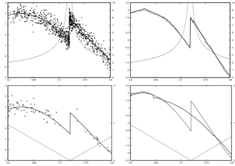
In figures5and6we give a more localized illustration of the heavysine dataset. We keep the same signal-to-noise ratio and sample size. We consider the design density
µ(x) = β+ 1 xβ0+1+ (1−x0)β+1 x−x0β1[0,1](x), (6.1) forx0 = 0.2,0.72 andβ =−0.5,1. -8 -6 -4 -2 0 2 4 6 0 0.05 0.1 0.15 0.2 0.25 0.3 0.35 0.4 0 1 2 3 4 5 6 7 8 9 10 -8 -6 -4 -2 0 2 4 6 0 0.05 0.1 0.15 0.2 0.25 0.3 0.35 0.4 0 1 2 3 4 5 6 7 8 9 10 -8 -6 -4 -2 0 2 4 6 0 0.05 0.1 0.15 0.2 0.25 0.3 0.35 0.4 0 1 2 3 -8 -6 -4 -2 0 2 4 0 0.05 0.1 0.15 0.2 0.25 0.3 0.35 0.4 0 1 2 3
Figure 5. Heavysine datasets and estimates with design density (6.1) with
x0= 0.2 and β =−0.5 at top, β= 1 at bottom.
-4 -3 -2 -1 0 1 2 3 0.6 0.65 0.7 0.75 0.8 0 1 2 3 4 5 6 7 8 9 10 -2.5 -2 -1.5 -1 -0.5 0 0.5 1 1.5 2 2.5 0.6 0.65 0.7 0.75 0.8 0 1 2 3 4 5 6 7 8 9 10 -3 -2 -1 0 1 2 3 4 0.6 0.65 0.7 0.75 0.8 0 1 2 -2.5 -2 -1.5 -1 -0.5 0 0.5 1 1.5 2 2.5 0.6 0.65 0.7 0.75 0.8 0 1 2
Figure 6. Heavysine datasets and estimates with design density (6.1) with
7. Proofs
7.1. Preparatory results and proof of theorem 1. The next lemma is a version of the bias-variance decomposition of the local polynomial estimator, which is classical: see for instanceFan and Gijbels(1995,1996),Goldenshluger and Nemirovski(1997),Spokoiny
(1998) and Tsybakov (2003), among others. The next lemmas are used within the proof of theorem 1, and are proven below. We recall that ΩI =
λ(XI) > (nµ¯n(I))−1/2 , see section2.1, that oscf stands for the local oscillation off, see (3.2), and that the matrixGI is defined in (3.5).
Lemma 1 (Bias variance decomposition). If I is such that µ¯n(I)>0 and x0 ∈I, we have
onΩI that
|fbI(x0)−f(x0)|62(K+ 1)1/2λ(GI)−1 oscf(I) +σ(nµ¯n(I))−1/2|γI|
, (7.1)
where γI is, conditionally on XI, centered Gaussian with Enf,µ{γI2|Xn}61.
We introducem(p, σ) := (2/π)1/2RR+(1+σt)pexp(−t2/2)dt. The next lemma shows that
the estimator cannot be too large in expectation.
Lemma 2. When kfk∞<+∞, we have for any p >0 andJ ⊂[0,1]:
Enf,µ|fbJ(x0)|p|Xn 6(K+ 1)p/2m(p, σ)(kfk∞∨1)p nµ¯n(J)p/2.
The next lemmas deal with the adaptive selection of the bandwidth. In particular, lemma3is of special importance, since it provides a control on the probability for a smooth-ing parameter to be selected by the procedure. Let us introduce
TI,J,m:=
|hfbJ −fbI, φmiJ|6σkφmkJTn(I, J) ,
and TI,J := ∩06m6KTI,J,m, TI :=∩J∈In(I)TI,J, where In(I) :={J ⊂I s.t. J ∈ In}. Note
that onTI, the bandwidthI is selected if it maximises ¯µn(I). Lemma 3. If I ∈ In is such that
oscf(I)6σDI ̺nµ¯n(I) −1/2
,
where we recall that DI is a tuning constant from the threshold term (2.6) and that ̺n =
n/logn, we have on ΩI∩ nµ¯n(I)>2 : Pnf,µ{TIc|Xn}6#(In(I))(K+ 1)(nµ¯n(I))−D 2 p/8,
where we recall thatDp = 4(p+ 1)1/2 (see (2.6))and where#(E) denotes the cardinal of E. Lemma 4. Let I ∈ In and J ∈ In(I). On the event TI,J∩ΩJ, we have
|fbI(x0)−fbJ(x0)|6(K+ 1)1/2λ(GJ)−1(DI+DpCK)σ ̺nµ¯n(J) −1/2
,
where we recall thatGJ is given by (3.5).
Proof of theorem 1. Letj be such thatx0 ∈[X(j), X(j+1)], where X(i)< X(i+1) for any
16i6n(eventually, we take X(0) := 0 andX(n+1) := 1). We consider the largest interval
In,f− inIn such thatIn,f− ⊂In,f. Since oscf(I)2µ¯n(I) increases as I increases, we have oscf(In,f− )6σDI ̺nµ¯n(In,f− )−1/2,
thus ¯µn In,f−
6µ¯n I¯n,f
. Ifp and q are such that
where a >1 is the grid parameter (see (2.8)), and if u, v are such that [X(u), X(v)]⊂In,f and ¯µn([X(u), X(v)]) = ¯µn(In,f), we have ¯ µn [X(j+1−[ap]), X(j+[aq])]6µ¯n [X(u), X(v)] 6µ¯n [X(j+1−[ap+1]), X(j+[aq+1])] , thus ¯µn In,f 6a2µ¯ n In,f− 6a2µ¯ n I¯n,f , and ¯ µn In,f/a2 6µ¯n I¯n,f6µ¯n In,f. (7.2) Note that for the grid choice given by (2.8), we have
#(In(I))6 log(nµ¯n(I))/loga2. (7.3) We introduce Tn :=
¯
µn( ¯In,f) 6µ¯n(Ibn) . By definition of Ibn we have Tcn ⊂ TI¯cn,f. Using
lemmas2,3 and (7.2), (7.3), we obtain: Enf,µ R−1 n,f|fbn(x0)−f(x0)| p 1Tc n|Xn 6(2p−1∨1)R−pn,f En f,µ |fbn(x0)|2p|Xn 1/2+kfkp∞ Pn f,µ{TI¯cn,f|Xn}1/2 6C(σ, a, p, K)(kfk∞∨1)plog nµ¯n( ¯In,f)1−p/2(nµ¯n( ¯In,f))p−D 2 p/16 6C(σ, a, p, K)(kfk∞∨1)p,
where C(σ, a, p, K) :=σ−p(2p−1 ∨1)(K+ 1)1+p/2m(2p, σ)1/2ap/loga and where we recall thatDp= 4(p+ 1)1/2.
By the definition ofIbn, we have
Tn⊂ TIbn,I¯n,f,
thus using lemma4 and (7.2), we obtain that on Tn,
|fbIb
n(x0)−fbI¯n,f(x0)|6λ
−1(G ¯
In,f)(DI+DpCK)aRn,f.
In view of lemma1 and definition (3.4) of ¯In,f, we obtain using again (7.2):
|fbI¯n,f(x0)−f(x0)|6λ(GI¯n,f)−1(K+ 1)1/2 oscf( ¯In,f) +σ(nµ¯n( ¯In,f))−1/2|γI¯n,f|
6λ(GI¯n,f)−1(K+ 1)1/2 DI+ (logn)−1/2|γI¯n,f|aRn,f,
where γI¯n,f is, conditionally on Xn, centered Gaussian and such that Enf,µ{γI2¯n,f|Xn} 6 1. Then, we have on Tn
Rn,f−1|fbn(x0)−f(x0)|6λ(GI¯n,f)−1(K+ 1)1/2a 3DI+DpCK+ (logn)−1/2|γI¯nn,f|,
and the theorem follows by integrating with respect toPn
f,µ(·|Xn).
7.2. Preparatory results and proof of theorem 2. Let us denote by Pnµ the joint probability of the variables Xi, 16 i6 n and let us recall the notation µ(I) =RIµ(t)dt. The next lemmas are used within the proof of theorem2, their proofs can be found below. Lemma 5. For any I ⊂[0,1], ε >0, we have:
Pnµ|µ¯n(I)/µ(I)−1|> ε 62 exp − ε 2 1 +ε/3nµ(I) .
Lemma 6. If µ satisfies (3.7), ω ∈RV(s) and rn =rn(ω, µ) is given by (3.8) and (3.9),
we have
rn∼P(s, β, σ,1)(logn/n)s/(1+2s+β)ℓω,µ(logn/n) as n→+∞, (7.4)
where ℓω,µ ∈ RV(0) is characterised by ω and µ and where we recall that P(s, β, σ, L) =
σ2s/(1+2s+β)L(β+1)/(1+2s+β). When ω(h) =Lhs,L >0 (H¨older smoothness), we have more
precisely:
rn∼P(σ, β, σ, L)(logn/n)s/(1+2s+β)ℓω,µ(logn/n) as n→+∞. (7.5)
We need to introduce some notations. Ifα∈N,h >0 and ifε >0, we define the event Dn,α(ε, h) := 1 µ(Ih) Z Ih · −x0 h α dµ¯n−gα,β 6ε ,
wherega,b:= (1 + (−1)a)(b+ 1)/(2(a+b+ 1)). The next lemmas are specifically linked with the uniform control of the smallest eigenvalue of the matrixΛIX¯IΛI, defined by (3.5). Lemma 7. If µ satisfies (3.7), we have for any positive sequence (γn) going to 0 and any
α∈N, ε >0: PnµDn,α(ε, γn)c 62 exp− ε 2 8(1 +ε/3)nµ(Iγn) , (7.6)
whenn is large enough.
We recall thathn=hn(ω, µ) is defined by (3.8). In what follows, we omit the dependence uponω and µto avoid overloaded notations. We introduce
Hn:= argmin h∈[0,1]
ω(h)>σ(̺nµ¯n(Ih))−1/2 , (7.7) which is an approximation of hn when µ is unknown. The next lemma controls the way howHn and hn are close. If 0< ε <1, we introduce the event
Cn(ε) :={(1−ε)hn< Hn6(1 +ε)hn}.
Lemma 8. If ω ∈RV(s), s >0 then for any 0 < ε2 61/2 there exists 0< ε3 6ε2 such
that forn large enough
Dn,0(ε3,(1−ε2)hn)∩Dn,0(ε3,(1 +ε2)hn)⊂Cn(ε2).
Let us denote Gn := GIHn and introduce the symmetrical matrix G with entries, for 06p, q6K:
(G)p,q:=
(1 + (−1)p+q)(2p+β+ 1)1/2(2q+β+ 1)1/2
2(p+q+β+ 1) .
This matrix is the limit (in probability) ofGn asn→+∞. It is easy to see that λ(G)>0: note thatG =ΛXΛ whereΛ= diag(1 +β)1/2,(2 +β)1/2, . . . ,(2K+ 1 +β)1/2, which is clearly invertible, andXhas entries (X)p,q = (1+(−1)p+q)/(2(p+q+β+1)) for 06p, q6K. Let us define the vector p(t) = (1, t, . . . , tk). Then, we haveλ(X)>0: otherwise,
0 =λ(X) =hx,Xxi= Z 1
−1
(x′p(t))2|t|βdt,
where x ∈ RK+1 is non-zero vector, which leads to a contradiction, since t 7→ x′p(t) is a polynomial (x′ stands for the transposition of x). Let us introduce the events An(ε) :=
|λ(Gn)−λ(G)|6ε forε >0 and forα∈N
Bn,α(ε) := µ(I1 hn) Z IHn · −x0 hn α dµ¯n−gα,β 6ε ,
which differs from Dn,α(ε, hn) since the integral is taken overIHn instead ofIhn.
Lemma 9. If ω ∈RV(s), s > 0 and µ satisfies (3.7), we can find for any 0< ε 61/2 an event An(ε)∈Xn such that
An(ε)⊂An(ε)∩Bn,0(ε)∩Cn(ε) (7.8)
for nlarge enough, and
PnµAn(ε)c 64(K+ 2) exp −DAr−n2
, (7.9)
where rn:=rn(ω, µ) is given by (3.9) and DA >0.
Proof of theorem 2. The proof of this theorem is based on the proof of theorem 1 and the previous lemmas. In the same fashion as in the proof of theorem 1, where we replace only equation (7.3) by
#(In(I))6 nµ¯n(I) 2
since the grid choice is (3.10) instead of (2.8), we obtain that on ΩIHn ∩
nµ¯n(IHn)>2 : Enf,µ R−1 n,f|fbn(x0)−f(x0)| p |Xn 6Aλ(GIHn) −p+B(kfk ∞∨1)p,
where we recall thatHnis defined by (7.7). Let us defineε:= min(ρ−1, λ/2) and consider the eventAn(ε) from lemma9. On this event, sinceAn(ε)⊂Cn(ε), we haveδn>(1+ε)hn>
Hn, thusf ∈ Fδ(ω, Q) entails that we have either
oscf(IHn)6ω(Hn) =σ ̺nµ¯n(IHn) −1/2 , or oscf(IHn)6ω(Hn)6σ (nµ¯n(IHn)−1)/logn −1/2 ,
which entails that in both cases oscf(IHn) 6 σDI ̺nµ¯n(IHn)
−1/2 since DI > √2, and that ¯ µn(IHn)6µ¯n(In,f). (7.10) Note that Bn,0(ε) =
|µ¯n(IHn)/µ(Ihn)−1|6ε . Thus, onAn(ε), we have in view of (3.8),
(3.9), (7.8) and (7.10) that rn(ω, µ)−1 6(1−ε)−1Rn,f−1, andnµ¯n(In,f)>(1−ε)nµ(Ihn)→
+∞ as n→ +∞, thus An(ε) ⊂ ΩIHn ∩
nµ¯n(IHn) > 2 . Then, since An(ε) ⊂An(ε), we
have uniformly forf ∈ Fδ(ω, Q):
Enf,µ rn(ω, µ)−1|fbn(x0)−f(x0)|p1A
n(ε) 6(1−ε)
−p/2(A(λ
−ε)−p+B(Q∨1)p).
Now we work on the complementary An(ε)c. Using lemma 2 and (7.9), we obtain that uniformly forf ∈ Fδ(ω, Q): En f,µ rn−1|fbn(x0)−f(x0)| p 1An(ε)c 6(2p−1∨1)r−pn h Enf,µ|fbn(x0)|2p 1/2+Qp i Pnµ{An(ε)c}1/2 6(2p−1∨1)(Q∨1)p(1 + (K+ 1)p/2m(σ,2p)1/2)rn−pnp/2 Pnµ{An(ε)c}1/2 =on(1), which entails (3.11). Moreover, (3.12) follows from lemma6, which concludes the proof.
The next lemma is a technical tool for computing the explicits examples given in sec-tion3.4. The proof can be found in Ga¨ıffas(2004).
Lemma 10. Let a∈Rand b >0. If G(h) =hb(log(1/h))a, then we have
7.3. Proofs of the lemmas. In the following, we denote byPI the projection in the space
VK for the scalar product h·,·iI which is given by (2.1). Note that on ΩI, we have (see section (2.1))
b
fI = ¯fI =PIY, (7.11) where PI is the projection in VK with respect to h·,·iI. We denote respectively by h·,·i and byk · k the Euclidean scalar product and the Euclidean norm inRK+1. We denote by
k · k∞ the sup norm inRK+1. We definee1 := (1,0, . . . ,0)∈RK+1.
Proof of lemma 1. On ΩI, we have X¯I =XI andλ(XI)>(nµ¯n(I))−1/2>0, thusXI is invertible. SinceΛI is clearly invertible on this event, GI is also invertible. By definition of oscf(I), we can find a polynomialPIε∈VK such that
sup x∈I|
f(x)−PIε(x)|6oscf(I) +ε/√n,
for any fixedε >0. If we denote byθI the coefficients vector of PIε then
|fbI(x0)−f(x0)|6|hΛI−1(θbI−θI), e1i|+ oscf(I) +ε/√n
=|hGI−1ΛIXI(θbI−θI), e1i|+ oscf(I) +ε/√n.
In view of (2.3), we have on ΩI form= 0, . . . , K:
(XI(θbI−θI))m =hfbI−PIε, φmiI =hY −PIε, φmiI
=hf −PIε, φmiI+hξ , φmiI=:BI,m+VI,m,
thus the decomposition into bias and variance termsXI(θbI−θI) =BI+VI, and
|fbI(x0)−f(x0)|6|hGI−1ΛIBI, e1i|+|hGI−1ΛIVI, e1i|+ oscf(I) +ε/√n.
We have
|hGI−1ΛIBI, e1i|6kGI−1ΛIBIk6kGI−1kkΛIBIk6kGI−1k(K+ 1)1/2kΛIBIk∞, and for 06m6K,
|(ΛIBI)m|=kφmk−1|hf−PIε, φmiI|6kf −PIεkI6oscf(I) +ε/√n. Sinceλ(M)−1=kM−1k for any symmetrical and positive matrixM, and sincekΛ−1
I k61, we have on ΩI: kGI−1k=kΛ−I1X−I1Λ−I1k6kXI−1k=λ(XI)−1 6(nµ¯n(I))1/2 6n1/2, thus |hGI−1ΛIBI, e1i|6(K+ 1)1/2 kGI−1koscf(I) +ε .
Conditionally onXn, the random vectorVI is centered Gaussian with covariance matrix
σ2(nµ¯n(I))−1XI. ThusGI−1ΛIVI is again centered Gaussian, with covariance matrix
σ2(nµ¯n(I))−1GI−1ΛIXIΛIGI−1 =σ2(nµ¯n(I))−1GI−1,
andhG−I1ΛIVI, e1i is then centered Gaussian with variance
σ2(nµ¯n(I))−1he1,GI−1e1i6σ2(nµ¯n(I))−1kG−I1k.
Since GI is positive symmetrical and its entries are smaller than one in absolute value,
kG−I1k = λ(GI)−1 and λ(GI) = infkxk=1hx ,GIxi 6 kGIe1k 6 (K+ 1)1/2. Thus kGI−1k 6
Proof of lemma 2. If ¯µn(J) = 0, we havefbJ = 0 by definition and the result is obvious, thus we assume ¯µn(J) > 0. Since λ(X¯J) > (nµ¯n(J))−1/2 > 0, X¯J and ΛJ are invertible andGJ also is. Thus,
b
fJ(x0) =hΛ−J1θbJ, e1i=hGJ−1ΛJX¯JbθJ, e1i=hGJ−1ΛJYJ, e1i.
For any 06m6K, we have
|(ΛJYJ)m|6kφmkJ−1 |hf , φmiJ|+|hξ , φmiJ|
6kfkJ+kφmk−J1|hξ , φmiJ|
6kfk∞+kφmk−J1|hξ , φmiJ|=:kfk∞+|VJ,m|.
Conditionally on Xn, the vector VJ with entries (VJ,m; 0 6 m 6K) is centered Gaussian with varianceσ2 nµ¯n(J)
−1
ΛJXJΛJ, thusGJ−1VJ is also centered Gaussian, with variance
σ2 nµ¯n(J)−1GJ−1ΛJXJΛJGJ−1=σ2 nµ¯n(J)−1Λ−J1X¯J−1XJX¯−J1Λ−J1.
The variablehGJ−1VJ, e1i is then, conditionally on Xn, centered Gaussian with variance
σ2 nµ¯n(J)−1he1,ΛJ−1X¯−J1XJX¯−J1Λ−J1e1i6σ2 nµ¯n(J)−1kΛJ−1k2kX¯−J1k2kXJk,
and since clearly kXJk 6 K + 1, kΛJ−1k 6 1 and kX¯J−1k = λ(X¯J)−1 6 nµ¯n(J) 1/2
, the variance of hGJ−1VJ, e1i is, conditionally on Xn, smaller than σ2(K + 1). Moreover,
kGJ−1k6kΛ−J1kkX¯J−1kkΛ−J1k6 nµ¯n(J) 1/2
, thus
|fbJ(x0)|6(K+ 1)1/2(kfk∞∨1) nµ¯n(J)1/2 1 +σ|γJ|,
where γJ is, conditionally on Xn, centered Gaussian with variance smaller than 1. The lemma follows by integrating with respect toPn
f,µ(·|Xn).
Proof of lemma 3. Let 06m6K and J ∈ In(I). In view of (2.3) and (7.11), we have on ΩI: hfbJ −fbI, φmiJ =hY −fbI, φmiJ =hf −fbI, φmiJ +hξ , φmiJ =hf −PIf , φmiJ+hPIf−fbI, φmiJ+hξ , φmiJ =hf −PIf , φmiJ+hPI(f −Y), φmiJ +hξ , φmiJ =hf −PIf , φmiJ− hPIξ , φmiJ+hξ , φmiJ :=A+B+C.
The termAis a bias term. By the definition of oscf(I) we can find a polynomialPIε∈VK such that
sup x∈I|
f(x)−PIε(x)|6oscf(I) +εn,
where εn := σDpCKlog 2/(4n). Thus, since J ⊂ I, PIε ∈ VK and PI is an orthogonal projection with respect toh·,·iI,
|A|6kf−PIfkJkφmkJ 6kf −PIε−PI(f−PIε)kIkφmkJ 6kf −PIεkIkφmkJ 6(oscf(I) +εn)kφmkJ, and by assumption, |A|6kφmkJ σDI(̺nµ¯n(I))−1/2+εn . (7.12)
Conditionally onXn,B and Care centered Gaussian. Clearly, C is centered Gaussian with
variance
σ2kφmk2J/(nµ¯n(I)).
Since PIξ has covariance matrix σ2PIP′I = σ2PI (PI is an orthogonal projection), the variance ofB is equal to En f,µ hPIξ , φmi2J|Xn 6kφmk2JEnf,µ{kPIξk2J|Xn} =kφmk2JTr Var(PIξ|Xn) /(nµ¯n(J)) =σ2kφmk2JTr(PI)/(nµ¯n(J)),
where Tr(M) stands for the trace of a matrix M. Since PI is the projection on VK, it follows that Tr(PI)6K+ 1, and that the variance of B is smaller than
σ2kφmk2J(K+ 1)/(nµ¯n(J)).
Then,
Enf,µ{(B+C)2|Xn}6σ2kφmk2JCK2/(nµ¯n(J)), (7.13) where we recall thatCK = 1 + (K+ 1)1/2. Sincenµ¯n(I)>2 by assumption, and ¯µn(J)61, we have εn6σDpCK log nµ¯n(I) / 4nµ¯n(J) 1/2 . (7.14)
Then, equations (7.12), (7.14) and the definition of the threshold (2.6) together entail kφmk−J1|hfbI−fbJ, φmiJ|> Tn(I, J) ⊂n kφmk −1 J |B+C| σ(nµ¯n(J))−1/2CK > Dp log(nµ¯n(I)) 1/2 /2o. Then, since TI,Jc = K [ m=0 kφmk−J1|hfbI−fbJ, φmiJ|> Tn(I, J) ,
we obtain using (7.13) and the fact that P{|N(0,1)|> x}6exp(−x2/2):
Pn f,µ{TIc|Xn}6 X J∈In(I) K X m=0 exp(−D2plog(nµ¯n(I))/8) 6#(In(I))(K+ 1)(nµ¯n(I))−Dp2/8,
which concludes the lemma.
Proof of lemma 4. Let us define HJ :=ΛJXJ. On ΩJ, we have:
|fbI(x0)−fbJ(x0)|=|(θbI−θbJ)0|6kΛJ−1(θbI−θbJ)k∞
6kGJ−1HJ(θbI−θbJ)k∞
6(K+ 1)1/2λ(GJ)−1kHJ(θbI−θbJ)k∞.
Since on ΩJ,hfbI−fbJ, φmiJ/kφmkJ = (HJ(bθI−θbJ))m, and sinceJ ⊂I, we obtain that on
TI,J:
|fbI(x0)−fbJ(x0)|6(K+ 1)1/2λ(GJ)−1Tn(I, J)
6(K+ 1)1/2λ(GJ)−1σ(DI+DpCK) ̺nµ¯n(J)) −1/2
,
Proof of lemma 5. It suffices to use the Bernstein inequality to the sum of independent random variables Zi=1Xi∈I−µ(I) for 16i6n.
Proof of lemma 6. Let us defineG(h) :=ω2(h)µ(Ih). In view of (3.7), we have µ(Ih) = 2R0hµ(x0+t)dt forh 6ν, andµ(Ih)∈ RV(β+ 1) sinceβ >−1 (see appendix), thus G∈ RV(1 + 2s+β). The functionGis continuous and going to 0 ash→0+since 1 + 2s+β >0, see (A.2). Thus, we have for n large enough hn = G←(σ2̺−n1) where G←(h) := inf{y > 0|G(y)>h}is the generalized inverse ofG. SinceG←∈RV(1/(1 + 2s+β)) (see appendix) we have ω◦G← ∈ RV(s/(1 + 2s+β)) and we can write ω◦G←(h) = hs/(1+2s+β)ℓ
ω,µ(h) whereℓω,µis slowly varying. In particular, we have ℓω,µ(σ2̺n−1)∼ℓω,µ(̺−n1), thus
rn=ω◦G←(σ2̺−n1)∼P(s, β, σ,1)(logn/n)s/(1+2s+β)ℓω,µ(logn/n) as n→+∞.
When ω(h) = Lhs we can write more precisely hn = G← (σ/L)2̺−n1
where G(h) =
h2sµ(Ih), and we obtain (7.5) in the same fashion as (7.4). Proof of lemma7. Let us defineQi := Xiγ−xn 0α1Xi∈Iγn andZi :=Qi−Enµ{Qi}. In view of (3.7), we can findN such that γn6ν for anyn>N and:
1 µ(Iγn) En µ{Qi}= 1 + (−1)α 2 γnβ+1ℓµ(γn) Rγn 0 tβℓµ(t)dt Rγn 0 tα+βℓµ(t)dt γnα+β+1ℓµ(γn) ,
where forh 6 ν, ℓµ(h) = h−βµ(x0+h) =h−βµ(x0−h) is slowly varying (see appendix).
Then, we have in view of (A.3): lim n→+∞
1
µ(Iγn)
Enµ{Qi}=gα,β, which entails that forn large enough:
Dn,α(ε, γn)c⊂ 1 nµ(Iγn) n X i=1 Zi > ε/2 . (7.15) Not that Enµ{Zi} = 0, |Zi| 6 2, Pni=1Enµ{Z2
i} 6 nEnµ{Q2i} 6 nµ(Iγn) and that the Zi,
16i6n are independent. Thus, we apply Bernstein inequality to the sum of theZi and
the lemma follows.
Proof of lemma 8. In view of (7.7), we have
Hn6(1 +ε2)hn =̺nµ¯n(I(1+ε2)hn)>σ
2ω((1 +ε2)hn)−2 .
We introduceε3:= minε2,1−(1−ε22)−2(1 +ε2)−2s, which is positive forε2 small enough, andℓω(h) :=h−sω(h) which is slowly varying, sinceω∈RV(s). Since (A.1) holds uniformly over each compact set in (0,+∞), we have for any y∈[1/2,3/2]
(1−ε22)ℓω(hn)6ℓω(yhn)6(1 +ε22)ℓω(hn) (7.16) for n large enough, so (7.16) with y = 1 +ε (ε 6 1/2) entails in view of (3.8) and since
h7→µ(Ih) is increasing: (1−ε3)̺nµ(I(1+ε2)hn)>(1−ε 2 2)−2(1 +ε2)−2sσ2ω(hn)−2 =σ2 (1 +ε2)hn−2s(1−ε22)−2ℓω(hn)−2 >σ2ω((1 +ε2)hn)−2. Thus ¯ µn(I(1+ε2)hn)>(1−ε3)µ((1 +ε2)hn) ⊂ Hn6(1 +ε2)hn ,
and similarly on the other side, we have forn large enough:
¯
µn(I(1−ε2)hn)6(1 +ε3)µ((1−ε2)hn) ⊂ {(1−ε2)hn< Hn},
thus the lemma.
Proof of lemma 9. Since Gn and G are symmetrical, we get \
06p,q6K
(Gn− G)p,q
6ε/(K+ 1)2 ⊂An(ε),
where we used the fact thatλ(M) = infkxk=1hx , M xifor any symmetrical matrixM. Then, an easy computation shows that ifε1 := min
ε, ε(β+ 1)/((K+ 1)2(2K+β+ 1)), we have for any 06p, q6K: Bn,p+q(ε1)∩Bn,2p(ε1)∩Bn,2q(ε1)⊂(Gn− G)p,q 6ε/(K+ 1)2 , and then 2K \ α=0 Bn,α(ε1)⊂An(ε).
Let us defineε2:=ε1/(2(1 +ε1)2K+1) and letε3 be such that (1 +ε3)β+3/(1−ε3)61 +ε2
and 0< ε3 6ε2. Sinceh7→µ¯n(Ih) is increasing, we have Cn(ε3)⊂
¯
µn(I(1−ε3)hn)6µ¯n(IHn)6µ¯n(I(1+ε3)hn) ,
and using lemma8, we can find 0< ε46ε3 such that
Dn,0(ε4,(1−ε3)hn)∩Dn,0(ε4,(1 +ε3)hn)⊂Cn(ε3).
In view of (A.1) and since ℓµ(h) := h−(β+1)µ(Ih) is slowly varying, we have for any 0 <
ε3 61/2:
ℓµ((1 +ε3)hn)6(1 +ε3)ℓµ(hn) andℓµ((1−ε3)hn)>(1−ε3)ℓµ(hn) (7.17) asnis large enough, thus simple algebra and the previous embeddings entail
Dn,0(ε4,(1−ε3)hn)∩Dn,0(ε4,(1 +ε3)hn)∩Dn,0(ε3, hn)⊂n ¯ µn(IHn) ¯ µn(Ihn) −16ε2 o .
Thus, in view of the previous embeddings, we have on Dn,0(ε4,(1−ε3)hn)∩Dn,0(ε4,(1 +
ε3)hn)∩Dn,0(ε3, hn): 1 µ(Ihn) Z IHn · −x0 hn α dµ¯n− Z Ihn · −x0 hn α dµ¯n 6 Hn∨hn hn αµ¯n(Ih n) µ(Ihn) µ¯n(IHn) ¯ µn(Ihn) −1 6(1 +ε3)α(1 +ε3)ε2 6(1 +ε1)2K+1ε2 =ε1/2.
Putting all the previous embeddings together, we obtain Dn,0(ε4,(1−ε3)hn)∩Dn,0(ε4,(1 +ε3)hn)
∩Dn,0(ε4, hn)∩Dn,α(ε1/2, hn)⊂Bn,α(ε1),
and finally, equation (7.8) follows if we take
An(ε) := Dn,0(ε4,(1−ε3)hn)∩Dn,0(ε4,(1 +ε3)hn)∩Dn,0(ε4, hn)
∩ \
06α62K
In view of (3.8), (3.9), (7.17), and since 0< ε3 61/2, we obtain using lemma7:
PnµAn(ε)c 64(K+ 2) exp −DArn−2
fornlarge enough, where DA := 2−(β+2)(σε4)2/(4(1 +ε4/3)), which concludes the proof of
the lemma.
7.4. Preparatory results and proof of theorem 3. The proof of theorem3 is similar to the proof of theorem 3 inBrown and Low(1996). It is based on the next theorem which can be found inCai et al.(2004). This result is a general constrained risk inequality which is useful for several statistical problems, for instance superefficiency, adaptation and so on.
Let p > 1 and q be such that 1/p+ 1/q = 1 and X be a real random variable having
distributionPθ with densityfθ. The parameterθcan take two valuesθ1 orθ2. We want to estimateθ based onX. The risk of an estimatorδ based on X is given by
Rp(δ, θ) :=Eθ{|δ(X)−θ|p}.
We defines(x) :=fθ2(x)/fθ1(x) and ∆ :=|θ2−θ1|. Let
Iq =Iq(θ1, θ2) := Eθ1{s
q(X)
}1/q.
Theorem 4 (Cai, Low and Zhao (2004)). If δ is such that Rp(δ, θ1) 6εp and if ∆> εIq,
we have: Rp(δ, θ2)>(∆−εIq)p >∆p 1−pεIq ∆ .
The next proposition is a generalization of a result by Brown and Low (1996) for the random design model, when the data is inhomogeneous. Of course, in the classical case withµcontinuous at x0 and such thatµ(x0)>0, the result is barely the same as inBrown and Low(1996) with the same rates. This proposition is a lower bound for a superefficient estimator which implies directly the adaptive lower bound stated in theorem3. Let us recall thatan is the minimax rate andαn is the minimax adaptive rate overA, see section4.2. Proposition 1. If an estimator fen based on (1.1) is asymptotically minimax over A, that
is:
limsupnsup f∈A
Enf,µ a−n1|fen(x0)−f(x0)|p <+∞,
and if this estimator is superefficient at a functionf0 ∈A, in the sense that for some γ >0:
limsupnEnf
0,µ
a−n1nγ|fen(x0)−f0(x0)|p <+∞, (7.18)
then we can find another functionf1 ∈A such that
liminfninf e fn En f1,µ α−n1|fen(x0)−f1(x0)| p >0.
Proof of proposition 1. Since limsupnEf
0,µ
a−n1nγ|fen(x0)−f0(x0)|
p
= C < +∞,
there isN such that for any n>N:
Ef0,µ |fen(x0)−f0(x0)|p 62Capnn−γp.
Let k′ = ⌊s′⌋ be the largest integer smaller than s′. Let g be k′ times differentiable with support included in [−1,1], g(0)> 0 and such that for any |x|6δ, |g(k′)(x)−g(k′)(0)|6
k′!|x|s′−k′. Such a function clearly exists. We define
f1(x) :=f0(x) +L′ρs ′ ng x−x0 ρn ,
whereρn is the smallest solution to
L′hs′ =σ ̺nµ(Ih)/b−1/2,
where b = 2g−∞2(p−1)γ, g∞ := supx|g(x)| and where we recall that ̺n = n/logn. We clearly havef1 ∈A. Let Pn0,Pn1 be the joint laws of the observations (1.1) when respectively f =f0,f =f1. A sufficient statistic for{Pn0,Pn1}is given by Tn:= log dPn0/dPn1
, and Tn∼ N −vn 2 , vn underPn0, N vn 2 , vn underPn 1, where, by definition ofρn: vn= n σ2kf0−f1k 2 L2(µ) = n σ2 Z (f0(x)−f1(x))2µ(x)dx 6nL′2ρ2ns′µ(Iρn)g 2 ∞/σ2 = 2(p−1)γlogn. An easy computation givesIq = exp vn(q−1)/2
6nγ, thus takingδ=fbn(x0),θ2=f1(x0), θ1 =f0(x0) and ε=an entails using theorem4:
Rp(δ, θ2)> L′ρs ′ ng(0)−2Cann−γnγ p > L′ρsn′g(0)(1−on(1)) p , since limnan/ρs ′
n →0, and the theorem follows.
Proof of theorem 3. Theorem3 is an immediate consequence of proposition 1. Clearly,
B⊂Athus equations (4.3) and (4.4) entail thatfen is superefficient at any functionf0∈B.
More precisely,fen satisfies (7.18) with
γ = (s−s
′)(β+ 1)
2(1 + 2s′+β)(1 + 2s+β) >0
sincen−γℓ(1/n)→0 for anyℓ∈RV(0). The conclusion follows from proposition 1.
Appendix A. Some facts on regular variation
We recall here briefly some results about regularly varying functions. The results stated in this section can be found inBingham et al.(1989). In all the following, letℓbe a slowly varying function. An important fact is that the property
lim
h→0+ℓ(yh)/ℓ(h) = 1 (A.1)
actually holdsuniformly for y in any compact set of (0,+∞). If R1 ∈ RV(α1) and R2 ∈
RV(α2), we have R1×R2 ∈RV(α1+α2) andR1◦R2∈RV(α1×α2). IfR∈RV(γ) withγ ∈R− {0}, we have R(h)→ ( 0 ifγ >0, +∞ ifγ <0, (A.2) ash→0+. If γ >−1, we have: Z h 0 tγℓ(t)dt∼(1 +γ)−1h1+γℓ(h) as h→0+, (A.3)
and h 7→ R0htγℓ(t)dt is regularly varying with index 1 +γ. This result is known as the Karamata theorem. Let us define (R is continuous)
R←(y) = inf{h>0 such thatR(h)>y},
which is the generalized inverse of R. If R ∈ RV(γ) for some γ > 0, there exists R− ∈ RV(1/γ) such that
R(R−(h))∼R−(R(h))∼h ash→0+, (A.4) andR− is unique up to an asymptotic equivalence. Moreover, one version of R− is R←. Acknowledgements. I wish to thank my adviser Marc Hoffmann for helpful advices and encouragements.
References
Antoniadis, A., Gregoire, G.andVial, P. (1997). Random design wavelet curve smoothing.
Statistics and Probability Letters,35225–232.
Baraud, Y.(2002). Model selection for regression on a random design.ESAIM Probab. Statist.,6 127–146 (electronic).
Bingham, N. H., Goldie, C. M. and Teugels, J. L.(1989). Regular Variation. Encyclopedia of Mathematics and its Applications, Cambridge University Press.
Brown, L. and Cai, T. (1998). Wavelet shrinkage for nonequispaced samples. The Annals of Statistics,261783–1799.
Brown, L. D.and Low, M. G. (1996). A constrained risk inequality with applications to non-parametric functional estimations. The Annals of Statistics,24 2524–2535.
Buckley, M., Eagleson, G.andSilverman, B. (1988). The estimation of residual variance in nonparametric regression. Biometrika,75189–199.
Cai, T. T., Low, M. and Zhao, L. H. (2004). Tradeoffs between global and local risks in nonparametric function estimation. Tech. rep., Wharton, University of Pennsylvania, http://stat.wharton.upenn.edu/˜tcai/paper/html/Tradeoff.html.
Delouille, V., Simoens, J. and Von Sachs, R. (2004). Smooth design-adapted wavelets for nonparametric stochastic regression. Journal of the American Statistical Society,99 643–658.
Donoho, D.andJohnstone, I.(1994). Ideal spatial adaptation via wavelet shrinkage.Biometrika, 81425–455.
Fan, J.andGijbels, I.(1995). Data-driven bandwidth selection in local polynomial fitting: variable bandwidth and spatial adaptation.Journal of the Royal Statistical Society. Series B. Methodolog-ical,57371–394.
Fan, J.andGijbels, I. (1996). Local polynomial modelling and its applications. Monographs on Statistics and Applied Probability, Chapman & Hall, London.
Ga¨ıffas, S. (2004). Convergence rates for pointwise curve estimation with a degenerate de-sign. Mathematical Methods of Statistics. To appear, available at http://hal.ccsd.cnrs.fr/ccsd-00003086/en/.
Gasser, T., Sroka, L. and Jennen-Steinmetz (1986). Residual variance and residual pattern in nonlinear regression. Biometrika,73625–633.
Goldenshluger, A.andNemirovski, A. (1997). On spatially adaptive estimation of nonpara-metric regression. Mathematical Methods of Statistics,6135–170.
Kerkyacharian, G.andPicard, D.(2004). Regression in random design and warped wavelets.
Bernoulli,101053–1105.
Lepski, O. V. (1990). On a problem of adaptive estimation in Gaussian white noise. Theory of Probability and its Applications,35454–466.
Lepski, O. V.,Mammen, E.andSpokoiny, V. G.(1997). Optimal spatial adaptation to inhomo-geneous smoothness: an approach based on kernel estimates with variable bandwidth selectors.
Lepski, O. V.andSpokoiny, V. G.(1997). Optimal pointwise adaptive methods in nonparametric estimation. The Annals of Statistics,252512–2546.
Maxim, V.(2003). Restauration de signaux bruit´es sur des plans d’experience al´eatoires. Ph.D. thesis, Universit´e Joseph Fourier, Grenoble 1.
Spokoiny, V. G.(1998). Estimation of a function with discontinuities via local polynomial fit with an adaptive window choice. The Annals of Statistics,261356–1378.
Stone, C. J.(1980). Optimal rates of convergence for nonparametric estimators. The Annals of Statistics,81348–1360.
Tsybakov, A.(2003). Introduction l’estimation non-paramtrique. Springer.
Wong, M.-Y.and Zheng, Z.(2002). Wavelet threshold estimation of a regression function with random design. 80 256–284.
Laboratoire de Probabilit´es et Mod`eles Al´eatoires, U.M.R. CNRS 7599 and Universit´e Paris 7, 175 rue du Chevaleret, 75013 Paris