Bayesian Learning Strategies in Wireless Networks

(1)

Università degli Studi di Padova

Dipartimento di Ingegneria dell’Informazione

Corso di Dottorato in Ingegneria dell’Informazione

Curriculum: Scienza e Tecnologia dell’Informazione

Ciclo: XXXI

Bayesian Learning Strategies

in Wireless Networks

Coordinatore:

Ch.mo. Prof. Andrea Neviani

Supervisore:

Ch.mo. Prof. Michele Rossi

Dottoranda:

Maria Scalabrin

(2)

(3)

Abstract

This thesis collects the research works I performed as a Ph.D. candidate, where the common thread running through all the works is Bayesian reasoning with applications in wireless networks. The pivotal role in Bayesian reasoning is inference: reasoning about what we don’t know, given what we know. When we make inference about the nature of the world, then we learn new features about the environment within which the agent gains experience, as this is what allows us to benefit from the gathered information, thus adapting to new conditions. As we leverage the gathered information, our belief about the environment should change to reflect our improved knowledge.

This thesis focuses on the probabilistic aspects of information processing with applications to the following topics: Machine learning based network analysis using millimeter-wave narrow-band energy traces; Bayesian forecast-ing and anomaly detection in vehicular monitorforecast-ing networks; Online power management strategies for energy harvesting mobile networks; Beam training and data transmission optimization in millimeter-wave vehicular networks. In these research works, we deal with pattern recognition aspects in real-world data via supervised/unsupervised learning methods (classification, forecasting and anomaly detection, multi-step ahead prediction via kernel methods). Fi-nally, the mathematical framework of Markov Decision Processes (MDPs), which also serves as the basis for reinforcement learning, is introduced, where Partially Observable MDPs use the notion of belief to make decisions about the state of the world in millimeter-wave vehicular networks.

The goal of this thesis is to investigate the considerable potential of infer-ence from insightful perspectives, detailing the mathematical framework and how Bayesian reasoning conveniently adapts to various research domains in wireless networks.

(4)

(5)

Sommario

Questa tesi raccoglie i lavori di ricerca svolti durante il mio percorso di dottorato, il cui filo conduttore è dato dal Bayesian reasoning con applicazioni in reti wireless. Il contributo fondamentale dato dal Bayesian reasoning sta nel fare deduzioni: ragionare riguardo a quello che non conosciamo, dato quello che conosciamo. Nel fare deduzioni riguardo alla natura delle cose, impari-amo nuove caratteristiche proprie dell’ambiente in cui l’agente fa esperienza, e questo è ciò che ci permette di fare uso dell’informazione acquisita, adattan-doci a nuove condizioni. Nel momento in cui facciamo uso dell’informazione acquisita, la nostra convinzione (belief) riguardo allo stato dell’ambiente cam-bia in modo tale da riflettere la nostra nuova conoscenza.

Questa tesi tratta degli aspetti probabilistici nel processare l’informazione con applicazioni nei seguenti ambiti di ricerca: Machine learning based network analysis using millimeter-wave narrow-band energy traces; Bayesian forecast-ing and anomaly detection in vehicular monitorforecast-ing networks; Online power management strategies for energy harvesting mobile networks; Beam-training and data transmission optimization in millimeter-wave vehicular networks. In questi lavori di ricerca studiamo aspetti di riconoscimento di pattern in dati reali attraverso metodi di supervised/unsupervised learning (classifica-tion, forecasting and anomaly detec(classifica-tion, multi-step ahead prediction via ker-nel methods). Infine, presentiamo il contesto matematico dei Markov Decision Processes (MDPs), il quale sta anche alla base del reinforcement learning, dove Partially Observable MDPs utilizzano il concetto probabilistico di con-vinzione (belief) al fine di prendere decisoni riguardo allo stato dell’ambiente in millimeter-wave vehicular networks.

Lo scopo di questa tesi è di investigare il considerevole potenziale nel fare deduzioni, andando a dettagliare il contesto matematico e come il modello probabilistico dato dal Bayesian reasoning si possa adattare agevolmente a vari ambiti di ricerca con applicazioni in reti wireless.

(6)

(7)

Acknowledgements

This thesis would not have been possible without the help of many people. First, I would like to express my sincere gratitude to my Ph.D. advisor Prof. Michele Rossi for the continuous support of my Ph.D, for his patience, motivation, and true passion for research. His guidance helped me in all the hard working times of research, with constructive criticism, precious advise, and moral support. This gave me uncountable opportunities for professional and personal growth. My sincere gratitude also goes to Prof. Nicolò Michelusi, who helped me to wisely widen my research skills from various stimulating perspectives. His enthusiastic attitude towards research has been inspirational. I would like to thank my friends and colleagues all over the world for sharing the most challenging, exciting, and intense moments of the last years together. I would like to thank my family: my parents, Anna, Roberto, and siblings, Sara, Giacomo, Elia, and Luca, for always being part of myself, wherever I am. Finally, last but not least, I would like to say a special thank to Emanuele, my ray of sunshine. Because I owe it all to you.

(8)

(9)

(10)

(11)

“Nothing in life is to be feared, it is only to be understood. Now is the time to understand more, so that we may fear less.”

(12)

(13)

List of Figures

2.1 Energy trace example of a DATA/ACK burst starting with a pair of beacons. . . 36 2.2 Example IEEE 802.11ad beam refinement sequence (top) and

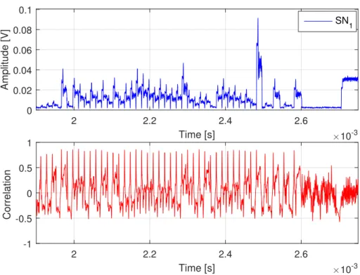
correlation coefficient (bottom) with respect to the beacon tem-plate. This BR sequence has 35energy levels. . . 37 2.3 Beam Refinement (BR) sequence of Fig. 2.2 (top) and

corre-sponding correlation coefficient (bottom) with respect to the beacon template. A correlation threshold (horizontal line in the bottom plot) is used to single out beacon messages (top graph), whereas the inter-beacon distance reveals whether a beacon is part of the BR sweep. The BR sequence has 35 energy levels and is correctly identified, see the green line in the top plot. . . 38 2.4 Flow diagram of the mm-wave channel pre-processing phase. . . 42 2.5 EDHMM training procedure: initial state duration estimates

are obtained through HMM training and are refined using EDHMM learning tools. . . 42 2.6 EDHMM runtime mm-wave channel analysis. . . 42 2.7 Synchronization using a variant of template matching, where a

subsequence from SN2 is used as a template. . . 46

2.8 Practical sniffer setup for trace capture. The antennas at the sniffers can be both directional or omni-directional, and sniffer location can be varied. . . 47 2.9 Communication recorded from two different locations SN1 and

(18)

2.10 Empirical measurements pdp_DATAMq , dp_ACKMq q for two marco-states. Rectangular regions are obtained using the Elbow method. Val-ues in the axes are expressed in number of channel samples (the sampling frequency isTs “0.1 µs). . . 58

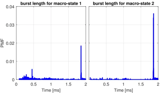
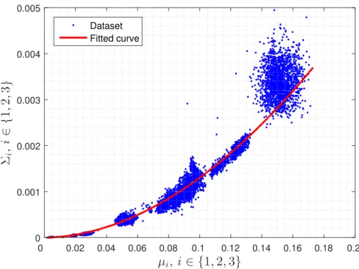
2.11 PMF of the burst length Ppdp_burstMq q for macro-models 1 and 2. . . 59 2.12 Gaussian observation model: empirical values and fitting curve

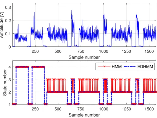
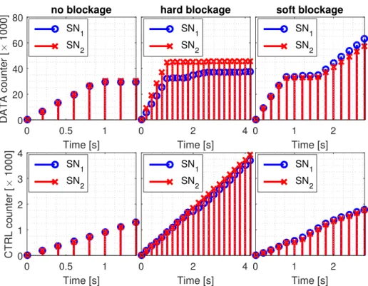
for mean (µ) and variance (Σ) of the received energy levels as-sociated with IDLE periods, DATA and ACK frames. . . 60 2.13 Trace decoding example for our machine learning framework. . . 61 2.14 Number of data and control packets identified by our tool. We

show the results for two sniffers SN1 and SN2 placed at different

locations. . . 62 2.15 CDF of packet and burst lengths for three links deployed in the

same environment but with varying performance. “BP” stands for beampattern. . . 63 2.16 Blockage recorded from two different locations SN1 and SN2.

The figure shows a fraction of the blockage, i.e., the blockage affects all samples. . . 64 2.17 Beam refinement sequences during soft link blockage. . . 65 2.18 Indoor measurement setup. Specifically, sniffers SN1 and SN2

are time-synchronized. . . 66 2.19 Number of data and control packets identified by our tool. The

results are for two sniffers SN1 and SN2 placed at different

lo-cations. The left plot shows the results from decoding the two traces independently; the results for the multi-dimensional trace (joint) processing are shown in the right plot. . . 67 2.20 ECDF of packet and burst lengths for the single trace and the

multi-dimensional (joint) trace processing (SN1 & SN2). . . 68

2.21 Estimated amplitude mean and standard deviation (std) of the EDHMM states i P t1,2,3u for the sniffers SN1 and SN2,

to-gether with other (omnidirectional) sniffers, as shown in the measurement setup of Fig. 2.18. . . 69

(19)

2.22 ρas a function of∆p1q_{, keeping}_∆p2q_{fixed for each curve. For this}

plot, µp₁dimq “ 0.001 for dim“1,2, the remaining energy levels follow from ∆pdimq_{, whereas the variances} _Σpdim_q

i are obtained

through Eq. (2.5). . . 70

2.23 ρ as a function of µp1q _with _∆p1q _“ _∆p2q _“ ₀_.₀₀₁_{, whereas} _µp1_q 1 and µp₁2q are allowed to change. . . 71

2.24 ρ as a function of µp1q _with _∆p1q _“ _∆p2q _“ ₀_.₀₀₂_{, whereas} _µp1q 1 and µp₁2q are allowed to change. . . 72

2.25 An example of sinusoidal noise which was found in the channel dynamics. The reconstructed signal is given as a sum ofN “3 sine waves, by looking at theN “3highest peaks in the Fourier transform of the trace. Specifically, the main component has frequency300 Hz, amplitude 0.0035 V. . . 73

2.26 ρin the presence of an additivesinusoidal noise with frequencyf. 74 3.1 Bayesian network associated with any target node in the phys-ical network topology. . . 81

3.2 PDF of the residual Respyt,yptq. . . 85

3.3 Complementary CDF of the residualRespyt,pytq. . . 86

3.4 Anomaly detection example for sensor node with ID 1000003 and cause nodes 1000003, 1000090, 1000197. . . 88

3.5 BN performance, when used as an anomaly classifier. . . 89

3.6 The ROC space. . . 91

4.1 Power packet grid topology. . . 95

4.2 Overview of the optimization framework. . . 96

4.3 Load pattern profiles (two classes). . . 105

4.4 One-step online forecasting for two weeks of data. . . 131

4.5 Multi-step prediction with different kernels. . . 132

4.6 Energy buffer levelvs cluster probabilityp. . . 133

4.7 Outage probability γptq vs cluster probabilityp. . . 133

4.8 Outage probability γptq over a day. . . 134

4.9 Purchased energyvs cluster probability p. . . 134

4.10 Outage probability γptq vs purchased energy threshold. . . 135

(20)

5.2 Rate and power as a function of λ and comparison with the heuristic πH for different pairs (PDT, TDT) (black crosses) and

PBVI with points inB˜obtained by random sampling (R). . . . 153 5.3 Rate and power as a function of λ, which is properly tuned

(21)

List of Tables

2.1 Average synchronization error versus template length τ. . . 45

4.1 List of symbols used in the chapter. . . 109

4.2 List of symbols used by the pattern analysis block. . . 110

4.3 List of symbols used by the optimization block. . . 111

4.4 AverageRMSEptq ˚ . . . 124

(22)

(23)

Chapter 1 Introduction

1.1 Motivation and Objectives

In the last decades we have seen a growing interest in Machine Learning. In the broadest sense, this field aims to learn new features about the environ-ment within which the agent gains experience. How gathered information is processed leads to the development of learning algorithms, i.e., how to process the collected data and deal with the uncertainty about the nature of the world. This thesis focuses on the probabilistic aspects of information processing with applications in wireless networks via Bayesian reasoning. The pivotal role in Bayesian reasoning is inference: reasoning about what we don’t know, given what we know. When we make inference about the nature of the world, then we learn new features about the environment within which the agent gains experience, as this is what allows us to benefit from the gathered information, thus adapting to new conditions. In this respect, Bayesian probability theory provides a mathematical framework for reasoning about the nature of the world in an effective, elegant, and precise fashion. When we make inference about the nature of the world, what we need is a means of discussing statements that have different levels of uncertainty. In other words, statements that have varying degrees of belief. In addition to modeling these statements within a mathematical framework, we want to be able to process the collected data. As we leverage the gathered information, our belief about the environment should change to reflect our improved knowledge. This is what defines learning.

(24)

1.2 Contributions

This thesis collects the research works I performed as a Ph.D. candidate, where the common thread running through all the works is Bayesian reasoning with applications in wireless networks. In the last decades we have seen a grow-ing interest in the design of adaptive models that exploit contextual informa-tion to enhance the overall network performance. In contrast to conveninforma-tional distributed optimization techniques, Machine Learning inspired mechanisms are able to operate in an online fashion, learning the current states of the wireless environment and the network’s users, improving the overall network performance over time. This, in turn, enables smarter network decision mak-ing, which is essential for most applications in wireless networks, particularly those that require real-time, low latency operations. The use of contextual information is also crucial to our analysis. Next, we provide an overview of the content of this thesis, which is organised in the following topics: Machine learn-ing based network analysis uslearn-ing millimeter-wave narrow-band energy traces; Bayesian forecasting and anomaly detection in vehicular monitoring networks; Online power management strategies for energy harvesting mobile networks; Beam training and data transmission optimization in millimeter-wave vehicu-lar networks. In particuvehicu-lar, while Chapters 2,3,4 deal with pattern recognition aspects in real-world data viasupervised/unsupervised learning methods (clas-sification, forecasting and anomaly detection, multi-step ahead prediction via kernel methods), Chapter 5 is different from the previous ones: here, the math-ematical framework of Markov Decision Processes (MDPs), which also serves as the basis for reinforcement learning, is introduced, where Partially Observ-able MDPs use the notion of belief to make decisions about the state of the world in millimeter-wave vehicular networks. Specifically, we are concerned with the problem of finding the optimal actions to take in a given situation in order to maximize a reward (or minimize a cost). Nowadays, reinforcement learning continues to be an active research area of Machine Learning. In this sense, even if Chapter 5 does not exploit state-of-the-art reinforcement solu-tions (where the agent gains experience while interacting with the environment, without prior knowledge of the exact mathematical model), it paves the way for pioneering research domains in millimeter-wave vehicular networks, where

(25)

deep reinforcement learning architectures can be designed to solve real-time optimization problems based on real-world data. Hereinafter, we provide an overview of the content of this thesis, in a chapter-by-chapter manner, detailing the mathematical framework and how Bayesian reasoning conveniently adapts to various research domains in wireless networks.

In Chapter 2, Hidden Markov Models (HMMs) and Explicit Duration HMMs (EDHMMs) are introduced to perform protocol frames classification in millimeter-wave wireless networks. Gaining information from spectrum usage is becoming important to provide smart adaptation capabilities to future net-work protocol stacks. Issues such as deafness, misaligned antennas, or blockage may severely impact network performance, and their identification is crucial. Despite the complexity of full analytical models, Machine Learning techniques are progressively being considered to improve spectrum usage at higher layers. In this chapter, we design a signal processing technique that uses narrowband physical layer energy traces, obtained from one or multiple channel sniffers. The proposed technique utilizes a combination of template matching and an EDHMM to correctly classify frames, while coping with the non-stationarity of the traces. This leads to a protocol level monitor that does not need to decode the channel at the physical layer, but just infers the type of packets that are exchanged based on sub-sampled energy traces. The performance of this framework is evaluated using off-the-shelf millimeter-wave wireless devices, quantifying its detection performance in the presence of one or multiple snif-fers, and assessing the impact of physical layer parameters such as noise power and signal levels. The idea is that different viewpoints of the same channel can provide diverse information and lead to higher decoding accuracies. We remark that our tool is the first automatic classifier of IEEE 802.11ad energy traces for network diagnosis. The uniqueness of our approach prevents direct comparison with earlier work. However, the resulting knowledge is extremely valuable, as it provides useful insights for network planners and administrators. In Chapter 3, Graphical Models are introduced to design a Bayesian fore-casting and anomaly detection framework for vehicular monitoring networks. This problem is tackled through localized and small-size Bayesian Networks (BNs), which are utilized to capture the spatio-temporal relationships under-pinning traffic data from nearby road links. A dedicated BN is set up, trained, and tested for each road in the monitored geographical map. The joint

(26)

prob-ability distribution between the cause nodes and the effect node in the BN is tracked through a Gaussian Mixture Model (GMM), whose parameters are es-timated via Bayesian Variational Inference (BVI) operating on unlabeled data. Optimal forecasting follows from the criterion of Minimum Mean Square Error (MMSE). Moreover, we also perform anomaly detection by devising a proba-bilistic score associated with the marginal conditional distribution of the effect node. The so obtained GMMs are time-dependent, i.e., several GMMs can be estimated for the same target road for different days of the weeks and/or hours of the day. Also, our framework is distributed, lightweight, and capable of op-erating in realtime and, in turn, it appears to be a promising candidate to deal with Internet of Things (IoT) applications in large-scale networks, where new data is to be processed on-the-fly. The effectiveness of the proposed framework is tested using a large dataset from a real network deployment, comparing its prediction performance with that of selected regression algorithms from the literature, while also quantifying its anomaly detection capabilities.

In Chapter 4, Gaussian Processes (GPs) are presented within the frame-work of Energy Cooperation and Model Predictive Control (MPC). The design of self-sustainable Base Station (BS) deployments is addressed in this chapter. We target deployments featuring small BSs with Energy Harvesting (EH) and storage capabilities. These BSs can use ambient energy to serve the local traffic or store it for later use. A dedicated power packet grid is utilized to transfer energy across them, compensating for imbalance in the harvested energy or in the traffic load. Some BSs are offgrid, i.e., they can only use the locally harvested energy and that transferred from other BSs, whereas others are on-grid, i.e., they can additionally purchase energy from the power grid. Within this setup, an optimization problem is formulated where: harvested energy and traffic processes are estimated (at runtime) at the BSs through GPs, and a MPC framework is devised for the computation of energy allocation and transfer across base stations. The combination of prediction and optimization tools leads to an efficient and online solution that automatically adapts to EH and load dynamics. Numerical results, obtained using real EH and traffic profiles, show substantial improvements with respect to the case where the optimization is carried out without predicting future system dynamics. The main improvements are in the outage probability (zero in most cases), and in the amount of energy purchased from the power grid, that is more than halved

(27)

for the same served load.

In Chapter 5, Partially Observable MDPs (POMDPs) use the notion of belief to make decisions about the state of the world in millimeter-wave ve-hicular networks. Future veve-hicular communication networks call for new so-lutions to support their capacity demands, by leveraging the potential of the millimeter-wave (mm-wave) spectrum. Mobility, in particular, poses severe challenges in their design, and as such shall be accounted for. A key question in mm-wave vehicular networks is how to optimize the trade-off between di-rective Data Transmission (DT) and directional Beam Training (BT), which enables it. In this chapter, learning tools are investigated to optimize this trade-off. In the proposed scenario, a Base Station (BS) uses BT to establish a mm-wave directive link towards a Mobile User (MU) moving along a road. To control the BT/DT trade-off, a POMDP is formulated, where the system state corresponds to the position of the MU within the road link. The goal is to maximize the number of bits delivered by the BS to the MU over the communication session, under a power constraint. In order to address the re-source constraints in our problem, we propose a Lagrangian method, and an online algorithm to optimize the Lagrangian variable based on the target cost constraint. Specifically, the Lagrangian variable is properly tuned within the main loop of the routine according to a gradient descent technique. Numerical results reveal that common-sense heuristic schemes cannot achieve the per-formance of the optimal policies, which take advantage of the belief update mechanism and provide adaptive BT/DT procedures according to the current belief, being able to maximize the transmission rate while showing robustness against BT errors.

(28)

(29)

Chapter 2 Machine Learning Based Network

Analysis using Millimeter-Wave

Narrow-Band Energy Traces

Next-generation wireless networks promise to provide extremely high data rates, especially exploiting the so-called millimeter-wave frequency range. Gain-ing information from spectrum usage is becomGain-ing important to provide smart adaptation capabilities to future network protocol stacks. Issues such as deaf-ness, misaligned antennas, or blockage may severely impact network perfor-mance, and their identification is crucial. Despite the complexity of full ana-lytical models, Machine Learning techniques are progressively being considered to improve spectrum usage at higher layers. In this chapter, we design a sig-nal processing technique that uses narrowband physical layer energy traces, obtained from one or multiple channel sniffers. The proposed technique uti-lizes a combination of template matching and an Explicit Duration Hidden Markov Model (EDHMM) to correctly classify frames, while coping with the non-stationarity of the traces. This leads to a protocol level monitor that does not need to decode the channel at the physical layer, but just infers the type of packets that are exchanged based on sub-sampled energy traces. The per-formance of this framework is evaluated using off-the-shelf millimeter-wave wireless devices, quantifying its detection performance in the presence of one or multiple sniffers, and assessing the impact of physical layer parameters such as noise power and signal levels.

(30)

2.1 Introduction

Next-generation wireless networks are called to provide extremely high data rates, especially exploiting the so-called millimeter-wave frequency range [1]. Applications and services will benefit from these high rates and the radio spectrum will become more and more densely utilized. As wireless networks turn into increasingly complex systems, accurate and scalable analytical mod-els to characterize their behavior are not yet available and very challenging to obtain. Instead, a promising approach is provided by machine learning tools that learn from data [2–4]. Gaining information from spectrum usage is deemed important to provide smart adaptation capabilities to future network protocol stacks. Possible applications include: (i) channel diagnosis: detect communication problems such as a link blockage, (ii) Quality of Service (QoS) tracking and adaptation, i.e., efficiently manage channel resources according to the detected energy level, (iii) information security: discovery of malicious signaling messages, etc.

As for the millimeter-wave (mm-wave) channel, its directional nature re-sults in communication issues that strongly impact higher layers, but which are hard to identify without detailed information of the underlying physical layer effects. This includes, e.g., deafness [5], misaligned antennas, and link blockage. Commercial Off-The-Shelf (COTS) devices are typically a black box regarding this physical layer information. As a result, troubleshooting COTS-based, real-world mm-wave network deployments often translates into time-consuming “trial-and-error” analysis. While understanding performance issues in such deployments is challenging [6–8], the resulting knowledge is ex-tremely valuable. It provides useful insights for network planners and admin-istrators. For instance, a missing acknowledgment after a data packet hints at a deafness issue, overlapping packet frames suggest a collision, and so on. However, gaining such insights from a COTS node that forms part of the net-work is virtually impossible. On top of the aforementioned lack of lower-layer access, a single node would be restricted to its particular point of view—the directivity of the communication limits the insights that one could gain. To prevent this, we need to capture and compare the behavior of the network from multiple viewpoints. Given the extreme bandwidth available in mm-wave

(31)

com-munications (e.g., 2 GHz per channel in the 60 GHz band), this requires an inordinate amount of data processing, and thus would be highly challenging.

In this chapter, we start filling the above identified gaps through the design and evaluation of an automatic tool for mm-wave channel analysis based on COTS hardware. Specifically, the tool uses machine learning techniques to in-fer protocol-level details such as packet types, their energy level and duration, and can help detect performance bottlenecks in 60 GHz networks using nar-rowband physical layer energy traces from one or multiple (omnidirectional) sniffers. That is, we do not record and decode the full communication but only require the energy level that the sniffers receive.

Our key contribution is developing a machine learning framework that correctly classifies the transmitted frame types (data, acknowledgements and training sequences) and can help infer network issues. This is far from triv-ial due to (a) the non-stationarity of the traces and (b) the complexity of the IEEE 802.11ad protocol [9]. To address (a), we dynamically update the parameters of the underlying machine learning model such that it adjusts to variations in the received energy level due to, e.g., node movement. Regard-ing (b), we use a combination of template matchRegard-ing and an Explicit Duration Hidden Markov Model (EDHMM) to correctly classify frames. The core idea of our approach is also applicable to networks operating at lower frequencies such as IEEE 802.11ac. Still, in this chapter we focus on the mm-wave case, which is more challenging due to the use of directional antennas and the large bandwidth. Since we do not need to decode any of the data, our approach preserves privacy, works regardless of whether the network uses encryption, and does not require accurate time/frequency synchronization. As a result, the proposed technique is simple yet highly effective. Our contributions are summarized as follows:

• _{We design a machine learning framework based on template matching}

and an EDHMM to automatically infer protocol layer information, e.g., transmitted packet types, their energy and duration, in 60 GHz net-works. The main challenge lies in the variability of the traces and in the complexity of identifying the structural elements in the traces given their noisiness, aperiodicity, and unpredictable behavior. Here, this is solved through a combination of statistical and machine learning techniques.

(32)

• We introduce a time-adaptive learning mechanism to cope with the non-stationarity of energy traces due to gain control adjustments and node movement. This run-time adaptation is barely explored in specialized work in the field of statistics but is critical for our approach. It also sets our scheme apart from existing work based on simple clustering or thresholding, which is highly sensitive to non-stationary behavior and thus often fails.

• We extend the learning framework to jointly process mm-wave channel traces from multiple time-synchronized sniffers. The idea is that different viewpoints of the same channel can provide diverse information and lead to higher decoding accuracies.

• We evaluate our approach in an extensive measurement campaign us-ing COTS 60 GHz hardware to analyze its performance in a range of practical scenarios. Besides, we numerically quantify the ability of the framework to correctly identify protocol sequences (beacon pairs, data and acknowledgment frames) from single and multiple channel sniffers, looking at the impact of channel noise and its distribution across different sniffers.

This chapter is organized as follows. The related work is surveyed in Sec-tion 2.2. In SecSec-tion 2.3, we discuss typical IEEE 802.11ad energy traces. Some mathematical background on the standard HMM and the extended EDHMM framework is provided in Section 2.4. The machine learning framework is in-troduced in Sections 2.5, 2.6, 2.7 and 2.8. In Section 2.9, this framework is generalized to perform decoding from multiple sniffers and a mm-wave channel trace generator that helps to evaluate the accuracy of our approach is presented in Section 2.10. We finally evaluate the proposed technique using experimen-tal and simulated energy traces in Section 4.5 and provide some concluding remarks in Section 2.12.

2.2 Related work

In the following, we give an overview of performance analysis and trou-bleshooting in mm-wave networking. As sketched in Section 2.1, mm-wave

(33)

networks suffer from high path-loss and high absorption. To overcome this, nodes typically use directional antennas and Line-Of-Sight (LOS) paths. How-ever, this makes links very susceptible to blockage. State-of-the-art work in this field [10–12] focuses on correctly identifying such blockage at the nodes involved in the communication, and reacting in a timely manner. For instance, BeamSpy [11] measures the set of available paths between a transmitter and a receiver. This “path skeleton” serves as a reference whenever blockage occurs— the nodes compute which of the paths in the skeleton is most likely to be unaffected by the blockage and steer their antennas accordingly. As a result, BeamSpy can avoid costly beam steering overhead. Further, earlier work by the same authors [12] looks into differentiating device movement from block-age based on Received Signal Strength (RSS) measurements. This is key to ensure that nodes react correctly when links degrade. Similarly, MOCA [10] transmits a very short control message to assess the link state. If the trans-mitter does not obtain a reply, it assumes that the antennas are misaligned. Otherwise, it adapts the Modulation and Coding Scheme (MCS) according to the current channel state. All of the above approaches aim at improving the performance of mm-wave networks. In contrast, our work troubleshoots the operation of such approaches and is thus orthogonal to them. While Beam-Spy and MOCA also try to identify specific issues in the communication, they are constrained to the specific “viewpoint” of a certain node. Our framework runs on one or more external sniffers which we can place at multiple locations, thus providing richer insights. Earlier work proposes an equivalent concept based on external sniffers. However, such approaches typically consider lower frequency bands, and focus on security issues [13, 14] such as realizing an In-trusion Detection System (IDS). The key difference to our study is that such security sniffers are designed to continuously operate along with the network, thus increasing the complexity of the deployment. In contrast, our tool does not need to be part of the network, and can be used on-demand only. Hence, we do not add complexity to the network. Moreover, we focus on performance issues in directional wireless networks while the above work deals with secu-rity in the omni-directional case. However, [14] and references therein also deal with raw physical layer data, similarly to our case. Specifically, they suggest overhearing the communication and jamming unwanted packets based on, for instance, header information. Our narrow band sniffer for wide band

(34)

signals also overhears the communication but does not (and in fact cannot) decode any preambles and headers to identify the packets. Instead, we use machine learning on the timing of frames from simple energy traces to obtain the information required for network analysis.

In recent years, machine learning techniques are increasingly being used to address high-dimensional problems with multiple unpredictable factors, e.g., for traffic classification, and previous papers typically use it after demodulating and decoding frames at the physical layer [15, 16] (although these approaches are not tailored to IEEE 802.11ad). In contrast, our framework uses ma-chine learning on the raw physical layer trace. Thus, it eliminates the need for the above operations, which are particularly complex and resource inten-sive in mm-wave networks and would require a sufficiently wide band channel sniffer. However, this poses additional challenges, such as identifying frames. In this chapter, we provide solutions to these challenges, which sets us apart from existing work. On top of the latest trends in wireless communications, machine learning based solutions for spectrum sensing/sharing in Cognitive Radio (CR) represent a promising approach for improving the utilization of the radio electromagnetic spectrum [17, 18]. To promote this, the Defence Advance Research Projects Agency (DARPA) [19] intends to develop tech-nologies for extensive spectrum sensing/sharing, both in the Radio Frequency Machine Learning Systems (RFMLS) program [2] as well as in another ma-jor DARPA effort known as the Spectrum Collaboration Challenge (SC2) [3], which is regarded as the first-of-its-kind collaborative machine-learning com-petition to overcome spectrum scarcity. Also the National Science Foundation (NSF) [4] is promoting projects to leverage machine learning solutions in CR. In the literature, automatic network recognition offers a promising framework for the integration of cognitive concepts at the network layer, bearing simi-larities with the mm-wave channel analyzer proposed in Section 2.5. In [20], the authors address the problem of automatic classification of technologies, with particular focus on Wi-Fi vs. Bluetooth recognition. Previous work, as for example [21], has addressed a related problem, allowing cooperative spec-trum sensing in peer-to-peer cognitive networks by using distributed detection theory [22] for identifying overlapping air interfaces based on time-frequency analysis and feature extraction. The same problem is tackled in [23], where two kinds of neural classifiers are adopted. Again, the authors focus on Wi-Fi

(35)

vs. Bluetooth recognition. While this work is related to ours, none of these studies perform protocol analysis from narrow band channel traces. We re-mark that our tool is the first automatic classifier of IEEE 802.11ad energy traces for network diagnosis. The uniqueness of our approach prevents direct comparison with earlier work.

2.3 A look into IEEE 802.11ad energy traces

The IEEE 802.11ad standard operates at 60 GHz. In this band, propa-gation conditions are worse than at lower bands, such as at 2.4 or 5 Ghz, which are used by the IEEE 802.11n/ac standards [24]. Specifically, the path loss is much higher at 60 GHz than at 2.4 or 5 GHz. To compensate for this attenuation, IEEE 802.11ad provides a mechanism for the establishment of a directional communication link between a transmitter/receiver pair using a beam training process. As a result of this process, the transmitting station focuses its energy towards the intended receiver. This compensates for the high path loss and reduces the potential interference to other stations that are located nearby.

IEEE 802.11ad divides the channel access into so called Beacon Intervals (BIs). Each BI is split into different access periods, which have different ac-cess rules and provide specific functionalities to the stations (STAs) within communication range. A typical BI is composed of a Beacon Header Inter-val (BHI) and a Data Transmission InterInter-val (DTI). The BHI contains several sub-intervals and is basically used to transmit control messages, such as bea-cons that enable beam training. In the DTI period, STAs exchange data frames either exploiting a contention-based access period or a scheduled ser-vice period. The former entails a contention mechanism (“floor acquisition”) to acquire the medium, which uses the enhanced distributed coordination func-tion. Conversely, in the scheduled service period, stations access the channel in a contention-free manner.

An example IEEE 802.11ad energy trace corresponding to a data exchange is shown in Fig. 2.1. This trace depicts the start of a typical data burst. The data burst starts with a pair of beacons which contain control information. This pair of beacons is followed by a sequence of data (DATA) packets and

(36)

250 500 750 1000 1250 1500 Sample number 0 0.1 0.2 0.3 A mplit ude [V

] Control Packets_{(Beacon Pair)} _{Data Packet and Acknowledgment Exchanges}

Figure 2.1: Energy trace example of a DATA/ACK burst starting with a pair of beacons.

acknowledgments (ACKs). In general, each DATA packet is followed by a corresponding ACK, which is the shorter packet in the figure and which has a higher energy level. Note that the higher amplitude of ACKs is due to the position of the sniffer, which in this case was near the receiver. The beam training process is composed of the following two phases.

• Sector Level Sweep (SLS). During the SLS, a STA selects a coarse grain antenna sector. This phase can be implemented in two ways: 1) through a transmit sector sweep (TXSS), i.e., a STA tries to select the best transmit antenna sector towards a particular receiving STA by trans-mitting Sector Sweep (SSW) frames using each of its antenna sectors or 2) through a receive sector sweep (RXSS), i.e., a receiving STA trains its receive antenna sector by requesting its peer STA to transmit SSW frames using a fixed antenna pattern, while the receiving STA sweeps across its receive antenna sectors.

• Beam Refinement (BR). To refine the sectors obtained in the SLS phase, multiple mechanisms are used. Basically, the two communicating STAs iteratively search for the optimal alignment starting from the coarse grain sector provided by the SLS. Occasional BR sequences retrain the antenna beams in case of, e.g., mobility, to ensure that both nodes remain in the boresight of each other.

Sequences of control packets are not difficult to identify within IEEE 802.11ad channel traces. The SLS sweeps that are used during the connection setup have

32different energy levels. The BR sequences, which are used for re-alignement, e.g., when there is a drop in the link quality, have35levels [25]. The particular

(37)

2 2.2 2.4 2.6 Time [s] _×10-3 0 0.02 0.04 0.06 0.08 0.1 Amplitude [V] SN₁ 2 2.2 2.4 2.6 Time [s] _×10-3 -1 -0.5 0 0.5 1 Correlation

Figure 2.2: Example IEEE 802.11ad beam refinement sequence (top) and cor-relation coefficient (bottom) with respect to the beacon template. This BR sequence has 35energy levels.

number of energy levels depends on the number of sectors of the antenna. Ex-isting hardware implements the above number of sectors. An example energy trace corresponding to a BR phase is shown in Fig. 2.2.

In general, it is not difficult to recognize the individual frame types (bea-cons, DATA, ACKs, and BR sweeps) in the energy traces by visual inspection. This enables one to infer the dynamics of the communication. For instance, a missing acknowledgment after a data packet hints at a deafness issue, over-lapping packet frames suggest a collision, and so on. However, while this is visually evident, manually inspecting the energy traces is infeasible given the number of packets when communicating at multi-gigabit-per-second rates. At the same time, recognizing frame types in an automated manner is hard. In this chapter, our goal is to devise and validate a technique for the au-tomatic identification and labeling of IEEE 802.11ad energy traces. Notably, BR/SLS sweeps can be reliably identified through a standard pattern matching technique, as we briefly describe next. Each sequence is composed of beacon frames, each having a different energy level, but all of them having the same

(38)

2 2.2 2.4 2.6 Time [s] _×10-3 0 0.02 0.04 0.06 0.08 0.1 Amplitude [V] SN₁ 2 2.2 2.4 2.6 Time [s] _×10-3 -1 -0.5 0 0.5 1 Correlation

Figure 2.3: Beam Refinement (BR) sequence of Fig. 2.2 (top) and correspond-ing correlation coefficient (bottom) with respect to the beacon template. A correlation threshold (horizontal line in the bottom plot) is used to single out beacon messages (top graph), whereas the inter-beacon distance reveals whether a beacon is part of the BR sweep. The BR sequence has 35 energy levels and is correctly identified, see the green line in the top plot.

(although noisy)distinctive shape. To capture this shape, we obtained a bea-con template, that is basically a smoothed out version of the beabea-cons that were measured experimentally. Hence, a standard convolution is performed between the input energy trace and the beacon template; for an example see the bottom plot in Fig. 2.2. As we show in Fig. 2.3, setting a proper threshold on the correlation signal allows one to single out the start of each beacon in the original sequence. It is then not difficult to check when exactly 32 or 35

properly spaced energy levels appear in a row and, in turn, detect the SLS/BR sweeps, see again Fig. 2.3. Further details on the template matching procedure are given in Section 2.6, whilst additional results on BR sequence detection are provided in Section 2.11.1.

While the identification of SLS/BR sweeps is doable through simple pro-cessing techniques, the characterization of DATA exchange phases is much more complex. In this case, we do not know in advance the duration of DATA

(39)

frames. Similarly, we do not know the number of DATA/ACK exchanges in the data burst. There may be missing ACKs and the energy levels of ACKs and DATA frames can be arbitrary, as they depend on the location of the sniffer with respect to the transmitter and the receiver. In addition, the start of each data burst has to be reliably identified, and the start and end points of each frame transmitted therein have to be reliably assessed as well. All of this leads to a sequential estimation problem that is the subject of the work that we expound in the following sections.

2.4 EDHMM preliminaries

Next, some mathematical background on the standard HMM and the ex-tended EDHMM framework is provided as a basis for the machine learning framework, which is introduced in Sections 2.5, 2.6, 2.7 and 2.8. Specifically, we demonstrate how the standard HMM is inadequate for our purpose. Still, we use it to calibrate the initial EDHMM.

We use uppercase and calligraphic fonts for sets, except for N_p_X;µ, σ2q, which refers to a Gaussian random variable X with mean µ and variance σ2. We denote a random sequence of lengthT byX1:T “ pX1, . . . , XTq, where the

random variable Xt at time index t P t1, . . . , Tu takes values in the set X,

with cardinality |X|. Realizations are indicated by lowercase letters, i.e., xt

is the realization ofXt, and with x1:T “ px1, . . . , xTq we denote a sequence of

realizations. Vectors are indicated by bold letters, e.g.,bbb, and we refer to their elements asbbb “ rb1, . . . , bKs, with|bbb| “K. For matrices we use uppercase bold

letters, e.g.,AAA “ taiju is a matrix with elements aij.

Markov models, whose states correspond to observable events, are inade-quate to solve our mm-wave channel estimation problem. The reason is that we measure a noisy version of the transmitted energy levels, as they are corrupted by random channel fluctuations. Instead, Hidden Markov Models (HMMs) [26] are a more appropriate tool, as their observations are probabilistic functions of the (hidden) state. Specifically, an HMM is composed of embedded stochastic processes, where an unobservable hidden random process is revealed to the observer through another set of random processes that produce the sequence of observations.

(40)

We now consider a data burst and aim to solve the following estimation problem. The observed channel samples in the data burst,O1:T “ pO1, . . . , OTq,

are modeled as a sequence of real-valued random variables corresponding to one of the following basic elements: “1” inter-frame space (IFS), “2” data packet (DATA) and “3” acknowledgement (ACK). Accordingly, the hidden stateStat

timetis a discrete random variable that can take values in the setS _{“ t}1,2,3u. We define S1:T “ pS1, . . . , STq as the sequence of random variables describing

the hidden states in the data burst, i.e.,t P t1, . . . , Tu. Our objective is then to reliably estimate the sequence of hidden states s1:T “ ps1, . . . , sTq from

obser-vations o1:T “ po1, . . . , oTq. The standard HMM makes two basic assumptions

regarding the embedded stochastic processes:

A1) The first assumption is that S1:T is a first-order Markov chain, i.e.,

PpSt`1|S1, . . . , Stq “PpSt`1|Stq. In particular, we have PpSt`1 “j|St“

iq “aij, whereAAA“ taiju,i, j PS, is the single-step transition probability

matrix of the HMM.1

A2) The second assumption is that the random variable Ot is statistically

independent ofpO1, . . . , Ot_´1q.2

Moreover, Ot is a probabilistic function of the hidden state St, i.e., it obeys

a suitable conditional probability PpOt|Stq and each random variable Ot can

use a private distribution PpOt|Stqover the hidden state. We use a Gaussian

observation model withPpOt|St “iq “ NpOt;µi, σi2q, where µi and σ2i specify

the mean and the variance of the random variable Ot, given that the hidden

state isiP S. This is known to well approximate the noise distribution for mm-wave channels [27]. For all hidden states iPS, we collect the parameter pairs

bi “ pµi, σi2q through vector bbb “ rb1, . . . , b|S_|s. We define πππ “ rπ1, . . . , π|S_|s, whereπi is the probability that the HMM is in stateiP S in the first time slot

of the burst. 1

Conversely, in the extended EDHMM, the entire process is not Markovian (memoryless). Instead the process is Markovian only at specified time instants.

2

Specifically, one observation per state is assumed in the standard HMM model while in the extended EDHMM each state emits a sequence of observations. The length of the sequence while in stateiPS is determined by the length of time spent in stateiPS, i.e., the durationd. Observations are assumed to be independent of timet, while in stateiPS. Also, in the extended EDHMM, the transition probabilityaijis independent of the duration

(41)

The HMM model is described through a further parameter vectorΘ_{“ r}_π_π_{π, A}_A_{A, bbb}_s_. Its maximum likelihood estimate given a sequence of observations is obtained through the Expectation-Maximization (EM) algorithm [28], which entails two-step iterations. Briefly, initial values forΘ_{are chosen, and using} assump-tions A1 and A2 the posterior distribution for the whole sequencePpS1:T|O1:T,Θq

is computed. Hence, this posterior is used to compute the expected log-likelihood (the Baum’s auxiliary function), QpΘnew_,Θ_q_{, as}

QpΘnew_,Θ_{q “} ÿ

S1:TPST

PpS1:T|O1:T,ΘqlogPpS1:T, O1:T|Θnewq, (2.1)

which is finally maximized with respect to Θnew_{, where} Θnew _{is the new} pa-rameter vector (HMM model) from the EM iteration. This process is repeated until convergence to a local maximum. A proper initialization ofΘ_(with par-ticular regard for bbb) is crucial for a good convergence of the EM algorithm. For a Gaussian-observation model, applying the two-step iterations of the EM algorithm is equivalent to using Baum’s re-estimation approach [29], which is as follows. Consider two new variablesξtpi, jq andγtpiq, with i, j P S, that are

defined as ξtpi, jq “ PpSt“i, St_`1 “j|O1:T,Θq and γtpiq “ ř| S_| j“1ξtpi, jq. We have: πnew_i “ γ1piq, anewij “ řT´1 t“1 ξtpi, jq řT´1 t“1 γtpiq µnew_i “ řT t“1γtpiqot řT t_“1γtpiq , σ_i2 new “ řT t“1γtpiqpot´µiq2 řT t_“1γtpiq (2.2) where ξtpi, jqand γtpiqare computed using the Forward-Backward algorithm,

see [30, 31].

We observe that the standard HMM is inadequate for our purpose. In fact, it uses a geometric Probability Mass Function (PMF) gpdq “ paiiqd´1p1´aiiq

to describe the dwell time of any hidden state St “iPS with self-transition

probability aii, i.e., gpdq is the probability of staying in any hidden state

St“iPS for d´1 subsequent time steps and then leave the state

(proba-bility p1´aiiq). It has been argued that this poorly models real

phenom-ena, since most real-life applications do not obey this temporally-decaying function [32]. To tackle this, we consider the Extended Duration Hidden

(42)

Figure 2.4: Flow diagram of the mm-wave channel pre-processing phase.

Figure 2.5: EDHMM training procedure: initial state duration estimates are obtained through HMM training and are refined using EDHMM learning tools. Markov Model (EDHMM), where for each hidden state iP S we have aii “0

and a state-specific distribution pipdq is defined over the discrete set Di “

tdmin

i , . . . , dmaxi u, where dmini and dmaxi are the minimum and maximum

dura-tions for the protocol element transmitted when the EDHMM is in state i, respectively. Hence, upon entering state i P S_{, the sequence of observations}

in that state is assumed to be conditionally independent (i.e., i.i.d. once the state is entered), of length d P D_i (sampled from pipdq), and is emitted from

PpOt|St“iq “NpOt;µi, σ2iq. For the EDHMM, the duration distributions are

collected into a vector ppp, withppp “ rp1p¨q, . . . , p|S_|p¨qs and the EDHMM is de-scribed through the parameter vector Θ_EDHMM _{“ r}_π_π_{π, A}_A_{A, bbb, p}_p_p_s_{. In the following} analysis, we use the HMM model to initialize the state duration distribution of the EDHMM (see Section 2.7 for further details on the EDHMM training). Also, we use the forward-backward algorithm proposed by Yu and Kobayashi in [33, 34], as an alternative and efficient approach to solve Eq. (2.2).

(43)

2.5 High level description of the framework

The aim of the mm-wave channel analyzer that we present in this chapter is twofold. First, we want to track when data bursts are transmitted and, for each, detect which packets are exchanged, their duration, and average energy. This allows to obtain statistics on their number, duration, whether there are channel problems (which may be detected from missing ACKs). As a second objective, we track the transmission of control packets, which are sent for link management purposes. These control packets appear in two flavors as follows:

C1) Beacon pairs that mark the beginning of a data burst. C2) BR sequences that are utilized to maintain the radio link. Our approach consists of three steps.

Step 1 – Pre-processing (Fig. 2.4): beacon detection and data burst ex-traction are implemented through the pre-processing chain of Fig. 2.4, which operates on the raw channel trace, through filtering, downsampling and tem-plate matching (see Section 2.6). We design the pre-processing chain for the case of 802.11ad but we can easily adapt it to suit other protocols. This pre-processing phase identifies all the beacons, classifies their occurrences into C1 and C2 and outputs a collection of N data bursts of the form top_1:n_Tq_n|n “

1, . . . , Nu, which are disjoint and contiguous channel subsequences.3

After Step 1, we delve into the semantic decoding of the protocol elements that are transmitted within each data burst, i.e., the elements in the above defined set S. To assess which elements are transmitted, along with their av-erage energy and timing, we utilize an EDHMM model, which is first trained (Fig. 2.5), and then used at runtime (Fig. 2.6) with non-stationary traces. Let yyy “ py1, y2, . . .q be a sequence of channel samples. In general, yyy can be

written as yyy “ xxx`www [35, Chapter 14], where xxx “ px1, x2, . . .q is the signal

of interest at the receiver, that is, after transmission, andwww “ pw1, w2, . . .q is

the background noise. From our experimental measurements, we know that

yyy is highly non-stationary across data bursts, i.e., there are substantial varia-tions in the energy associated with the signalxxx and the noisewww, which entail changes in µi and σ2i, for i P S. Moreover, they can also be caused by power

3

(44)

control adjustments to compensate for channel attenuation and device mobil-ity. Nevertheless, the transmission time of the elements in set S are channel and protocol-specific. We proceed through the following steps.

Step 2 – EDHMM training (Fig. 2.5): we use stationarychannel traces4

for a preliminary and robust training of the EDHMM parameters. Channel traces were picked so as to encompass a wide range of data rates and MCSs, which determine the different lengths of the physical layer data frames. The distance between transmitter and receiver is kept fixed and the surrounding environment (indoor for our experiments) is kept as stable as possible (i.e., no user mobility, etc.). From these stationary channels, the state-specific distri-butions pipdq for i P S do not undergo major changes during each trace and

this allows their accurate estimation. Then, all the trace-specific distributions are combined into a global distribution considering a wide range of protocol settings, see Section 2.7. Note that training is needed only once for a given technology (e.g., IEEE 802.11ad).

Step 3 – Runtime trace analysis (Fig. 2.6): the EDHMM parametersµi

and σ2

i, for i P S do depend on channel attenuation and noise. Thus, these

parameters are estimated at runtime for each data burst using a clustering algorithm, whereas thepipdqare known from Step 2. The so obtained EDHMM

model is used to estimate the most likely sequence in S (called the Viterbi path) from the samples in the current data burst. This step is explained in Section 2.8.

Steps 2 and 3 rely on the further assumption that:

A3) Channel attenuation and noise are stationary within bursts.

2.6 Pre-processing

Data acquisition, filtering, and downsampling: to obtain the energy traces that we use as input for our machine learning algorithm, we overhear the communication of COTS 60 GHz devices using one or more external sniffers. Each sniffer consists of a Sivers IMA FC1005V/00 V-Band converter. The

4

These stationary channel traces do not exhibit any particular trend. This means that

µi andσ2

(45)

Table 2.1: Average synchronization error versus template length τ.

τ “1 ms τ “2 ms τ “3 ms τ “4 ms τ ě5 ms

36.36 ms 13.43 ms 2.63 ms 1.17 ms 0

converter receives signals in the 60GHz band either via a directional (20˝_{) or}

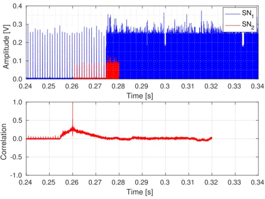
omni-directional antenna and outputs them at 2GHz intermediate frequency (IF). We capture the IF signal using a Universal Software Radio Peripheral (USRP) X310 Software Defined Radio (SDR) at a sample rate of30MHz. That is, we only need to capture afragmentof the bandwidth of the signal to obtain an energy trace which is suitable for our machine learning technique. To obtain a second trace from a different angle, we connect a second sniffer to the same USRP to ensure perfect time synchronization among traces. Since the coverage area of a mm-wave AP is limited due to high path loss, sniffers are typically close to each other and can thus be connected to the same USRP. Moreover, if traces are recorded on different USRPs, it is possible to synchronize them in post-processing using a variant of template matching, see Fig. 2.7, where a subsequence from SN2is used as a template. In Tab. 2.1, we report the average

synchronization error as a function of the template length τ. To obtain these results, we have run 1,000 simulations for each value of τ picking a random subsequence from SN1 and a subsequence from SN2 (used as a template) with

random temporal offset with respect to the subsequence from SN1. We obtain

perfect synchronization by choosing τ ě 5 ms. Synchronizing traces from multiple sniffers is thus doable and only requires picking a sufficiently long template length.

Fig. 2.8 shows our measurement setup. The original raw trace yyy is first filtered and then downsampled to a lower rate for scaling purposes, so that each sample of the new trace is computed as the mean of three subsequent samples in the original raw trace. This new trace is then smoothed using a fast and robust discretized spline filtering algorithm for data of large size [36] [37], thus obtaining the traceyyy˜. This pre-processing phase is needed to remove part of the noise due to hardware impairments during data acquisition. It does not harm the EDHMM classification performance, but generally improves it, as the noise variance in the energy traces is reduced.

Template matching algorithm: after the data acquisition, filtering, and downsampling, a collection of N data bursts of the form to_1:pn_Tq_n|n “1, . . . , Nu

(46)

0.24 0.25 0.26 0.27 0.28 0.29 0.3 0.31 0.32 0.33 0.34 Time [s] 0.0 0.1 0.2 0.3 0.4 Amplitude [V] SN₁ SN₂ 0.24 0.25 0.26 0.27 0.28 0.29 0.3 0.31 0.32 0.33 0.34 Time [s] -1.0 -0.5 0.0 0.5 1.0 Correlation

Figure 2.7: Synchronization using a variant of template matching, where a subsequence from SN2 is used as a template.

is extracted from the mm-wave traceyyy˜. This requires a reliable identification technique for the data bursts and, recalling that each data burst is preceded by a pair of beacons, this corresponds to reliably detecting beacon pairs. What we observe from the collected channel traces is that the beacon duration and the inter-frame spacing between them are almost constant within and across experiments. Moreover, we note that the beacon shape is quite particular, showing different energy levels at the beginning and at the end. These char-acteristics make it possible to exploit a template matching technique for the beacon detection. Here, we are interested in finding C1) beacon pairs, and C2) BR sequences, as these are key to understand the protocol behavior.

At the core of our template matching approach, we use Pearson’s correla-tion coefficientrP r´1,1s[38], which is a statistical measure of the strength of a linear relationship between two vectorsuuu“ ru1, . . . , uKsandvvv “ rv1, . . . , vKs

(with mean µu and µv, respectively). It is defined as the ratio of their

covari-ance Cuv and the square root of the product of their variances σ2u andσv2, i.e.,

(47)

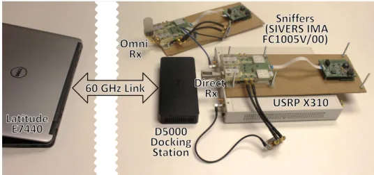
Figure 2.8: Practical sniffer setup for trace capture. The antennas at the sniffers can be both directional or omni-directional, and sniffer location can be varied. Cuv “ 1 K ´1 K ÿ k“1 puk´µuqpvk´µvq. (2.3)

Pearson’s correlation coefficient is suitable to deal with the non-stationarity of the traces, since it just evaluates some internal relationship between the pro-vided vectors. Moreover, template matching is known to be the optimal de-tection technique in the presence of white Gaussian noise [39], which we found to be a good assumption for our mm-wave channel traces [27]. Henceforth, for our template matching technique,uuu corresponds to the average shape of a beacon frame (i.e., the template with a length ofK samples), which the system can easily obtain from channel idle times. During those idle times, nodes only transmit periodic beacons which can be clearly identified and used as a tem-plate. Vectorvvv contains the channel samples from the current K-dimensional sliding window, which moves over the signal traceyyy˜, obtained after the acquisi-tion, filtering, and downsampling ofyyy. We adopted the fast template matching scheme of [40] [41], which exploits the Fast Fourier Transform (FFT), thus ob-taining dot products in the frequency domain. For a generic channel sequenceyyy˜

ofLąK samples, this allows the computation of the covariance inOpLlogLq

time. Hence, the template matching operates on yyy˜“ py˜1, . . . ,y˜Lq, outputting

a sequence of correlation estimatespr1, . . . , rL´K`1q. We detect a possible

(48)

matches (i.e., rℓ ąrth) are likely to occur within a window of samples, we

per-form a further peak detection within the regions containing multiple matches, by taking the default timing parameters of the IEEE 802.11ad communication standard into account [42]. That is, two beacons can never be placed at a distance smaller than the minimum allowed by the protocol rules. As the final step, we assess which beacon pairs actually mark the start of data bursts by assessing the distance between them, as this is constant. Through this, we can reliably detect false positives, such as isolated beacons due to communication errors or to packets that are erroneously detected as beacons as their shape closely resembles that of the template. We found excellent results across all our experiments setting rth “0.75. Note that rth is independent of the trace

amplitude. Thus, we do not need to readjust it for each scenario and/or trace. The identification of pairs of beacons (C1) allows extracting the data bursts

top_1:n_Tq_n|n“1, . . . , Nu fromyyy˜, which are fed as input to the following EDHMM training phase. Longer beacon sequences (C2) are likewise detected by looking at the number of energy levels of the beacons therein and at their inter-frame spacing, as dictated by the standard [42]. These events are semantically de-coded as described below.

2.7 EDHMM training

For the EDHMM training we refer to Fig. 2.5. We recall that the objective of this training phase is to reliably estimate the distribution vectorppp, modeling the duration of inter-frame spaces, packets and acknowledgements. This phase is executed once offline and is not scenario dependent. Essentially, it is a calibration step for the specific mm-wave technology used in the network, which in our case is IEEE 802.11ad. The traces used in this step should be as much as possible stationary. This means thatµi andσi2 do not significantly vary across

data bursts. As a first processing stage, we use the pre-processing procedure of Section 2.6, which returns the data burst settop_1:n_Tq_n|n“1, . . . , Nu. Next, for illustration purposes we refer to the n-th data burst op_1:n_Tq_n “ po1, . . . , oTnq, but in our implementation the HMM parameters are estimated using the entire burst set (i.e., the N bursts in the mm-wave trace). For burstn, each of the samples ot, t “ 0, . . . , Tn, maps to an element st P S, where state “1” means

(49)

IFS, “2” DATA and “3” ACK. Our goal is to accurately associate eachotin the

data burst with the actual protocol element i P S and, most importantly, to reliably estimate its duration PMF pip¨q. This estimation is performed having

access to the noisy observations po1, . . . , oTnq of the actual protocol elements. EDHMM initialization: we consider op_1:n_Tq_n as training data and our aim is to get accurate state duration estimates for the EDHMM. This is achieved by deriving initial estimates forpppthrough a simpler HMM model. Once this vector is found, it is refined using EDHMM training tools. The HMM parameter vector is Θ_HMM _{and the three fundamental steps involved in the HMM model} estimation are:

E1) The forward-backward algorithm is used to compute metrics γtpiq and

ξtpi, jqwith t“1, . . . , Tn,i, j P S (see Eq. (2.2)) for a given HMM

tran-sition structure and a list of observations. These weigh the probability of getting the observed sequence from the current model.

E2) The model parameter vector Θ_HMM _{is adjusted through the EM} algo-rithm.

E3) The Viterbi algorithm [43] is used to compute the most probable path via a Maximum Likelihood (ML) approach.

Step E2 returns the optimal parameter vectorΘ‹

HMM, whereas E3 outputs the

sequence of hidden statesps1, . . . , sTnqthat most likely generated the observed samplespo1, . . . , oTnq.

Specifically, we assume π1 “ 1 as all the data bursts start with a silence,

right after the beacon pair. Moreover, the HMM transition matrixAAA is con-strained in the sense that the hidden state sequence evolves according to struc-tured trajectories [44]. In particular, we have a23 “a32“0, as there must be

some minimum inter-frame spacing between subsequent messages. Also, we setaii“1´1{Ts for iP S, where Ts “0.1 µs is the channel sampling period

after the downsampling of Section 2.6. The initialization implies geometri-cally distributed state dwell-time distributions. This serves as a sufficiently good initialization of the transition matrix, and increases the robustness of the HMM model against random fluctuations in the channel dynamics. Next, we use the Viterbi algorithm output (step E3) to initialize the state duration distribution of the EDHMM model.