Reduced Model Based Control of Two Link Flexible Space Robot

(1)

Reduced Model Based Control of Two Link Flexible

Space Robot

Amit Kumar1, Pushparaj Mani Pathak2, Nagarajan Sukavanam1 1_{Department of Mathematics, Indian Institute of Technology Roorkee, Roorkee, India}

2_{Department of Mechanical and Industrial Engineering, Indian Institute of} Technology Roorkee, Roorkee, India

E-mail: tomardma@gmail.com, pushpfme@iitr.ernet.in, nsukvfma@iitr.ernet.in Received January 16, 2011; revised April 11, 2011; accepted April 15, 2011

Abstract

Model based control schemes use the inverse dynamics of the robot arm to produce the main torque compo-nent necessary for trajectory tracking. For model-based controller one is required to know the model pa-rameters accurately. This is a very difficult task especially if the manipulator is flexible. So a reduced model based controller has been developed, which requires only the information of space robot base velocity and link parameters. The flexible link is modeled as Euler Bernoulli beam. To simplify the analysis we have con-sidered Jacobian of rigid manipulator. Bond graph modeling is used to model the dynamics of the system and to devise the control strategy. The scheme has been verified using simulation for two links flexible space manipulator.

Keywords:Flexible Space Robots, Bond Graph Modeling, Reduced Model Based Controller, Euler-Bernoulli

Beam

1. Introduction

Space robots are a blend of a vehicle and a robot. It is mechanically more complex than a satellite. The flexible space robot will be useful for space application due to their light weight, less power requirement, ease of ma-neuverability and ease of transportability. Because of the light weight, they can be operated at high speed. For flexible manipulators flexibility of manipulator have considerable influence on its dynamic behaviors. It is observed by many researchers that fixed-gain linear con-trollers alone do not provide adequate dynamic perform-ance at high speeds for multi-degrees of-freedom robot manipulators. Out of various schemes studied so far, those involving the calculation of the actuator torque (force) using an inverse dynamics model (the computed torque methods), and those applying adaptive control techniques have been extensively studied, and show the greatest promise.

The traditional control strategy of robot manipulators is completely error driven and shows poor performance at high-speeds, when the high dynamic forces act as dis-turbances. The current trend is towards model-based control, where the dynamic forces are incorporated in the

control strategy as feed forward gains and feed-back compensations along with the servo-controller which is required only to take care of external noise and other factors not included in the dynamic model of the robot. As is expected, the model-based control scheme exhibits better performance, but demands higher computational load in real time. A particular area of model-based con-trol is adaptive concon-trol, which is useful when the dy-namic parameters of the robot are not well-known a pri-ori. The controller adapts itself during execution of tasks and improves the values of the dynamic parameters.

(2)

Wang and Gao [5] have reported inverse dynamics model-based control for flexible-link robots, based on modal analysis, i.e., on the assumption that the deforma-tion of the flexible-link can be written as a finite series expansion containing the elementary vibration modes. Leahy et al. [6] worked on robust model based control. They also discussed an experimental case. Fawaz et al. [7] developed a model based real-time virtual simulator of industrial robot in order to detect eventual external collision. The method concerns a model based fault de-tection and isolation used to determine any lock of mo-tion from an actuated robot joint after contact with static obstacles. Tso et al. [8] worked on a model-based control scheme for robot manipulators employing a variable structure control law in which the actuator dynamics is taken into consideration. Zhu et al. [9] attached an addi-tional model-based parallel-compensator to the conven-tional model-based computed torque controller which is in the form of a serial compensator to enhance the ro-bustness of robot manipulator control. Qu et al. [10] have discussed robust control of robots by the computed torque law with respect to unknown dynamics by judi-ciously choosing the feedback gains and the estimates of the nonlinear dynamics. The choices for the constant gains depend only on the coefficients of a polynomial bound of the unknown dynamics. Khosla and Kanade [11] presented the experimental results of the real-time per-formance of model-based control algorithms. The com-puted-torque scheme which utilizes the complete dy-namics model of the manipulator is compared with the independent joint control scheme which assumes a de-coupled and linear model of the manipulator dynamics. Pathak et al. [12] worked on a scheme for robust trajec-tory control of space robot and this work presents a re-duced modal based controller for trajectory control of flexible space robot in work space. Berger et al. [13] carried out the application of bond graph modeling to robots. Special emphasis is placed on adjusting the exact bond graph to allow for valid numerical solutions.

This paper presents a model based controller which requires the information of the base of space robot, link length, joint angle and evaluation of Jacobian. The con-troller is based on robust overwhelming control of the flexible space manipulator. To illustrate the methodology, an example of a two DOF flexible space robot is consid-ered. The controller is provided with tip velocity infor-mation of manipulator. Bond graphs are used to represent both rigid body and flexible dynamics of the link in a unified manner. The advantage of the bond graph is that it is used to model system, in multi energy domain and various control strategies can be devised using this mod-eling method. SYMBOLS Shakti [14] software is used for bond graph modeling and simulation.

2. Modeling of Two Arm Flexible Space

Robot

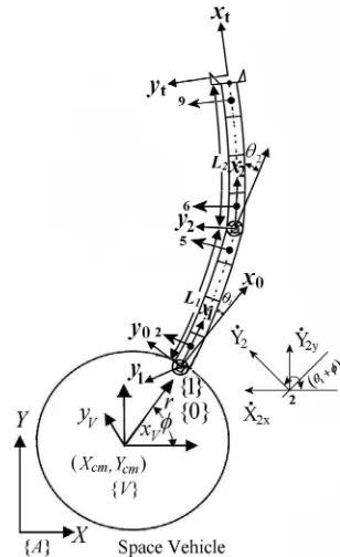
Let us assume that the space robot has single manipulator with revolute joints and is in open kinematic chain con-figuration. Figure 1 shows the schematic sketch of two arm flexible space robot. In this figure {A} represents the absolute frame, {V} represents the vehicle frame, {0} frame is located in space vehicle at the base of the robot, {1} frame is located in first arm at the base of first arm, {2} frames is located second joint. The frame {t} locates the tip of the robot. Let L1 be the length of the first link, L2 be the length of second link and r is the distance be-tween the robot base and center of mass (CM) of the space vehicle. Let the first motor is mounted on base and it applies a torque 1 on first link. Similarly let the sec-ond motor is mounted on first link and it applies a torque

2

 on second link. The cross section area of links are assumed to be A. The densities of first and second links are 1 and 2 respectively. The flexible links are uniform in cross section with flexural rigidities EI1 and EI2. The flexible link of space robot has been modeled as Euler-Bernoulli beam.

3. Bond Graph Modeling

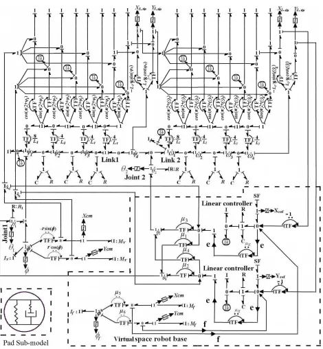
[image:2.595.343.497.437.689.2]

The kinematic analysis of flexible links is performed in order to draw the bond graph as shown in Figure 2. Fig-ure 2 also shows the pad sub model. From the kinematic

Figure 1. Schematic representation of two arm flexible pace robot.

(3)

[image:3.595.65.535.73.581.2]

Figure 2. Complete bond graph model of two arm flexible space robot with reduced model based controller. relations the different transformer moduli used in bond

graph model are derived. Two type of motion of the links are considered. First motion is the motion perpendicular to the link and second motion is the rotational motion of the links. The velocities in perpendicular to link is re-solved in X and Y direction.

In Figure 2, MV and IV represents the mass of space

vehicle and inertia of space vehicle. Let Xcm and Ycm be

the co-ordinate of the CM of the space vehicle with

re-spect to absolute frame. The first and second link is di-vided into four segments of equal length. The segment angles of first and second link are ψ1, ψ2, ψ3, ψ4 and ω1,

ω2, ω3, ω4 respectively. The segment inertias are at-tached to “1” junction structure corresponding to these velocities. Pads are used for computational simplicity i.e., to avoid the differential causality.

(4)

as







2x cm sin 2cos π 2

X  X  r  Y 1



(1)







2y cm cos 2sin π 2

Y Y  r  Y ₁



(2) where 1  1 , and Y2 is the velocity of the link in direction perpendicular to link at junction 2. The velocity of the first link tip in X and Y direction with respect to absolute frame can be evaluated as





  

_1 5 1 8 sin 4 4

t x

X  X  L   (3)



  

_1 5 1 8 cos 4 4

t y

Y Y  L  _ ₍₄₎

where X5x and Y5y are the velocity of the first link at

junction 5 in X and Y direction.



The velocity of the second link at junction 6 in X and Y direction with respect to absolute frame can be evalu-ated as



6x t_1 6cos π 2

X X Y 1



(5)





6y t_1 6sin π 2 1

Y Y Y  (6) where 6 is the velocity of second link at junction 6 in the direction perpendicular to link. The velocity of the robot at tip in X and Y direction with respect to absolute frame can be evaluated as

Y



  

_ 2 9 2 8 sin 4 4

t x

X X  L   (7)



  

_ 2 9 2 8 cos 4 4

t y

Y Y  L   (8) where X9x and Y9y are velocity of the link in X and Y

direction at junction 9.



From the above kinematic analysis different trans-former modulli used in drawing bond graph can be evaluated and are shown in Table 1.

4. Reduced Model-Based Controller Design

In work space control the robot is required to track a given end-effector trajectory, this is achieved by using a reduced model based controller. The bond graph model of a two DOF flexible planar space robot controller is shown in Figure 2. The model is represented in the iner-tial frame. Controller consists of three parts.

1) Space robot virtual base model 2) Overwhelming controller [12] 3) Jacobian.

4.1. Space Robot Virtual Base Model

[image:4.595.310.537.104.377.2]

A virtual base of the space vehicle is considered. To de-sign the model based controller, drawing analogy from the space vehicle, the tip velocity of manipulator in X and Y direction is considered in controller design. It is

Table 1. Transformer moduli for finding velocities at vari-ous points in bond graph model.

Description X Direction Y Direction

Robot Base TF = –r sin() TF = r cos()

First Segment of

First Link TF = cos(/2 + ψ1) TF = sin(/2 + ψ1)

Second Segment

of First Link TF = cos(/2 + ψ2) TF = sin(/2 + ψ2)

Third Segment

Fourth Segment

First Link Tip TF = – (L1/8) sin(ψ4) TF = (L1/8) cos(ψ4)

First Segment of

Second Link TF = cos(/2 + ω1) TF = sin(/2 + ω1)

Second Segment

of Second Link TF = cos(/2 + ω2) TF = sin(/2 + ω2)

Third Segment

Fourth Segment

Second Link Tip TF = – (L2/8) sin(ω4) TF = (L2/8) cos(ω4)

determined by translational inertia Mf of space vehicle.

The displacement relation of the robot are given as









1

2 1 2

cos cos

cos

tipf f f f

f

X X r L

L

1

  

  

   

   (9)









1

2 1 2

sin sin

sin

tipf f f f

f

Y Y r L

L

1

  

  

   

   (10)

Here f is the rotation of the space vehicle.

The tip velocity of the robot Xtipf , and due to

motion of the space vehicle can be found as, tipf

Y





















1 1

2 1 2

1 1 2 1 2

2 1 2 2

sin sin

sin

sin sin

sin

tipf f f f

f f

f

X X r L

L L L L        1            _       _    _     _   _   _      (11)





















1 1

2 1 2

1 1 2 1 2

2 1 2 2

cos cos

cos

cos cos

cos

tipf f f f

f f

f

Y Y r L

L L L L        1            _       _    _     _   _   _      (12)

[image:4.595.308.543.404.704.2]

(5)

ro-bot dynamics, then neglecting the coefficients of 1 and 2

 _{in Equations (11) and (12) we get,} modulli involve only link lengths and joint angles of the _manipulator.









1

2 1 2

sin sin

sin

tipf f f f

f f

X X r L

L 1          _       _  

 (13) 4.2. Overwhelming Controller

The linear overwhelming controller [12] is applied to the tip of the space robot model. The overwhelming control-ler is provided with reference velocity and tip velocity information. The effort signal produced by the controller is magnified by high gain and then the joint torques are evaluated with the help of Jacobian. This joint torque information is fed to different joints.









1

2 1 2

cos cos

cos

tipf f f f

f f

Y Y r L

L 1          _       _  

 (14)

Using Equation (13) and (14), the transformer modulli µ5, and µ6 shown in bond graph of Figure 2, can be writ-ten as,







5 rsin f L1sin f 1 L2sin f 1

  _         ₂



_



2

 _

4.3. Evaluation of Jacobian







6 rcos f L1cos f 1 L2cos f 1

 _         If we assume that the arms of manipulator are rigid then,

kinematic relations for the tip displacement Xtip,

in X and Y directions can be written as, tip Y One can observe from these expressions that these

















1 1 2 1

1 1 2 1 2

cos cos cos

sin sin sin

tip CM

X X r L L

Y Y r L L

                       _{ } _     _ _ _ _{ }       2  2 (15)

The tip angular displacement with respect to absolute

frame X axis is given as, lated in bond graph. For the planar case discussed here The Jacobian of the forward kinematics can be calcu-this relation can be worked out directly from Equation (15) as follows,

1

tip

      (16)

































1 1 1 2 1 2 1 2

sin sin sin

cos cos cos

tip CM

r L L

X X

Y Y r L L

                                     _{ } _      _{ } _               _ _        

        (17)









































1 1 2 1 2

1

1 2 2

1 2 2 ₂

sin cos

sin sin

cos cos

sin sin sin

cos cos cos

tip CM

X X r

Y Y r

L L

L L L

                             



                     _ _{ } _{ }              _{  }                             _{  }      (18)

For the evaluation of joint torque if we assume that

space vehicle rotational velocity , and CM velocity CM

X , CM are small, then neglecting the first and last

term of Equation (18) we get

Y

























1 2 2 1

1 2 2 2

1 1 2 1 2

sin sin sin

cos cos cos

tip

X L L L

Y L L L

                                     _ _{ } _{ }           

  (19)





3 L2sin 1 2 ,

      

 

1 2 tip tip X J Y                 

  (20)





4 L2cos 1 2 .

     

With the help of Equation (20) various transformer

modulli shown in bond graph can be evaluated as

_{5. Simulation and Results}

tation; first and second int angles are 0 radian, 0.5 radian and 0 radian

respec-





1 L1sin 1 L2sin 1 2



         

It is assumed that initially base ro







2 L1cos 1 L2cos 1 2



(6)

for the robot tip is a circle of radius R. Then the tip co

tively. Figure 3 shows the initial configuration of the space robot. At the beginning of the simulation over-whelmer initial position is initialized to robot tip posi-tion.

Let us assume that the reference displacement com-mand

ordinates will be given as,

 

cos

 

0

ref

X t  R t X (21)

 

sin

 

0

ref

Y t R t Y

Here

(22)

0 0

(X Y, )

he corresp

is the center of the circle. T onding reference vel

gi ,

circular reference ocity command is ven by

 

sin refx

f R t (23)

 

cos refy

f R t (24) At the start of simulation the refe

initialized to tip trajectory. The pa si

values used for simulation. rence trajectory is rameters used for mulation are shown in Table 2. The simulation is car-ried out for 1.56 seconds.

Table 2. Parameters and

Parameter Value

Modulus of E_lasticity E = 70 __{10 N/}9 _m2

Link Length

Figure 3. Initial configuration of two arm flexible space robot.

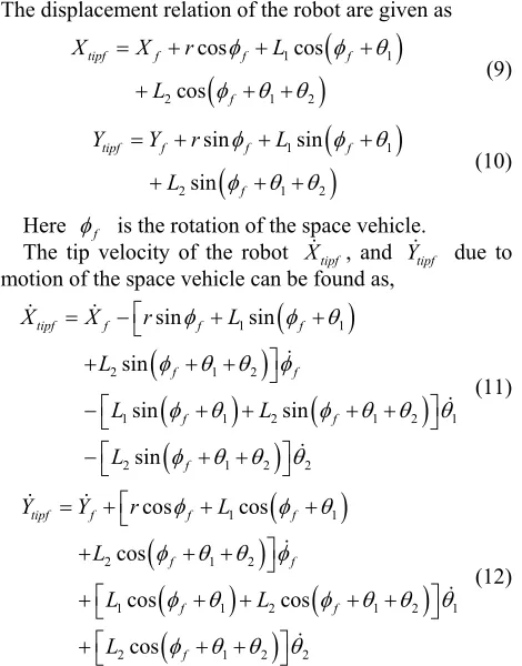
Figure 4(a) shows the plot for reference trajectory in

rection, Figure 4(c) shows the plot for tip trajec-ry in

this paper we presented a novel reduced model based ory control of flexible space robot in Bernoulli beam model is used to

x direction, Figure 4(b) shows the plot reference trajectory in y di

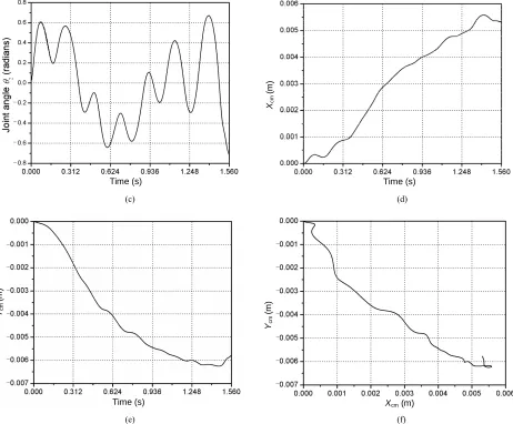
to x direction, and Figure 4(d) shows the plot for tip trajectory in y direction. From Figures 4(a) and (c) it is seen that tip follows the reference trajectory in x direc-tion and from Figures 4(b) and (d) it is also seen that tip follows trajectory in y direction effectively. Due to the nature of the flexible link tip vibration are observed. Figure 5(a) shows the plot of base rotation with respect to time. The base of the space vehicle rotates between the points 0.0 to –0.03 as the space robot is free floating. Figure 5(b) shows the plot of first joint angle with re-spect to time. Figure 5(c) shows the plot of second joint angle with respect to time Figure 5(d) shows the plot of CM of space vehicle in x direction with respect to time. Figure 5(e) shows the plot CM of space vehicle in y di-rection with respect to time. Figure 5(f) shows the plot of CM trajectory of space vehicle. Figures 5(d), (e) and (f) it is seen that there is continues movement in base of space robot as it is free floating.

Figure 6 shows the tip trajectory error plot. The error is taken as the difference between reference and actual tip position. Figure 6(a) shows the error plot for X tip position with respect to time. Fi

L L

obot Base CM

m

st A1 = 6.288 –5_m2_,

A2 = m2

R

Moment of Inertia of Space _I

Im1 = 0.001 kg·m2,

Im2 = ·m2

MC = 0. 0.13

Internal Damping Coeffi-terial

Input Reference Angular

Density of Aluminum ρ= 2700 kg/m3 1 = 0.5 m; 2 = 0.6 m

–13 4 Link Inertia I1 = 6.609  10 m ,

I2 = 6.609  10–13_m4

Location of R

fromVehicle r = 0.1 m

Mass of the First Link 1 = 1.0 kg

Cross Section Area of Fir

and Second Link 

10 6.288  10–5

Joint Resistances R_{2 = 0.0001 Nm/(rad/s)}1 = 0.001 Nm/(rad/s),

Mass of Base M = 5.0 kg

Vehicle V = 1.0 kg-m2

Gain Value µH = 8.0

Motor Inertias _{0.001 kg}

Controller 001, KC = 0.241, RC =

cient for Ma Rint = 0.01 N/(m/s)

Reference Circle Radius R = 0.400 m

Velocity  = 1.0 rad/s

gure 6(b) shows the er-ror plot for Y tip position with respect to time. From the simulation we see that initially error increases with time but after some time it start reducing.

6. Conclusions

In

controller for traject ork space. Euler w

(7)

Time (s)

Xre

f

(m

)

Time (s)

Yre

f

(m

)

(a) (b)

Time (s)

Xti

p

(m

)

Time (s)

Yti

p

(m

)

(c) (d)

Figure 4. (a) Reference trajectory in x direction; (b) Refer rajectory in y direction; (c) Tip trajectory in x direction d) Tip trajectory in y direction.

ence t . (

-

Time (s) Time (s)

[image:7.595.72.526.86.480.2]

(8)

-

Time (s) Time (s)

Xcm

(m

)

(c) (d)

-

Time (s)

Ycm

(m

)

-Ycm

(m

)

Xcm (m)

(e) (f)

Figure 5: (a) Plot of base rotation versus time; (b) Plot of first joint angle versus time; (c) Plot of second joint angle versus time; (d) Centre of mass trajectory in x direction; (e) Centre of mass trajectory in y direction; (f) Centre of mass trajectory of space vehicle.

-(a) (b)

[image:8.595.68.530.84.466.2]

(9)

of the reduced model based controller is that it does not require the link dynamic parameters and the trajectory tracking is very good. However the model has limitation as compared to analytical model as it is finite approxi-mation of continuous system. The future work will be focus on developing a reduced model based controller for three dimensional flexible space manipulator.

7. References

[1] Y. Murotsu, S. Tsujio, K. Senda and M. Hayashi, “Tra-jectory Control of Flexible Manipulators on a Free Flying Space Robot,” IEEE Control Systems, Vol. 12, No. 3, 1992, pp. 51-51.doi:10.1109/37.165517

[2] Y. Murotsu, K. Senda and M. Hayashi, “Some Trajectory Control Schemes for Flex

Flying Space Robot,” Proceedings of International Con-fer

ible Manipulators on a Free

ence on Intelligent Robots and Systems, Raleigh, 1992. [3] B. Samanta and S. Devasia, “Modeling and Control of

Flexible Manipulators Using Distributed Actuators: A Bond Graph Approach,” Proceedings of the IEEE Inter-national Workshop on Intelligent Robots and Systems, 1988.doi:10.1109/IROS.1988.592414

[4] B. Fardanesh and J. Rastegar, “A New Model Based Tracking Controller for Robot Manipulators Using the Trajectory Pattern Inverse Dynamics,” Proceedings of the

ternational Conference on Robotics and

ice, 1992.

doi:10.1109/ROBOT.1992.219938

1992 IEEE In Automation, N

, 2003.

on Robotics and Automation, Cincinnati, Vol. 3, 1990, pp. 1982-1987.

[7] K. Fawaz, R. Merzouki and B. Ould-Bouamama, “Model Based Real Time Monitoring for Collision Detection of an Industrial Robot,” Mechatronics, Vol. 19, No. 5, 2009, pp. 695-704. doi:10.1016/j.mechatronics.2009.02.005

[5] F. Y. Wang and Y. Gao, “Advanced Studies of Flexible Robotic Manipulators: Modeling, Design, Control and Application: Series in Intelligent Control and Intelligent Automation,” Word Scientific, New York

[6] M. B. Leahy Jr., D. E. Bossert and P. V. Whalen, “Robust Model-Based Control: An Experimental Case Study,”

Proceedings of the 1990 IEEE International Conference

[8] S. K. Tso, L. Law, Y. Xu and H. Y. Shum, “Implement-ing Model-Based Variable-Structure Controllers for Ro-bot Manipulators with Actuator Modeling,” Proceedings of the 1993 IEEE/IRSJ International Conference on Intel-ligent Robots and Systems, Yokohama, 1993.

doi:10.1109/IROS.1993.583137

[9] H. A. Zhu, C. L. Teo and G. S. Hong, “A Robust Model-Based Controller for Robot Manipulators,” P ro-ceedings of the IEEE International Symposium on Indus-trial Electronics, Vol. 1, 1992, pp. 380-384.

and D. M. Dawson, “Ro-e Law,” [10] Z. Qu, J. F. Dorsey, X. Zhang

bust Control of Robots by the Computed Torqu

Systems and Control Letters, Vol. 16, No.1, 1991, pp.25-32.doi:10.1016/0167-6911(91)90025-A

[11] P. K. Khosla and T. Kanade, “Real-Time Implementation and Evaluation of Computed-Torque Schemes,” IEEE Transactions on Robotics and Automation, Vol. 5, No.2, 1989, pp. 245-263.doi:10.1109/70.88047

[12] P. M. Pathak, R. Prasanth Kumar, A. Mukherjee and A. Dasgupta, “A Scheme for Robust Trajectory Control of Space Robots,” Simulation Modeling Practice and The-ory, Vol. 16, 2008, pp. 1337-1349.

doi:10.1016/j.simpat.2008.06.011

[13] R. M. Berger, H. A. EIMaraghy and W. H. EIMaraghy, “The Analysis of Simple Robots Using Bond Graphs,”

Journal of Manufacturing Systems, Vol. 9 No. 1, 2003, pp. 13-19, 2003.