Does model performance improve with complexity? A case study
with three hydrological models
Rene Orth
a,⇑, Maria Staudinger
b, Sonia I. Seneviratne
a, Jan Seibert
b, Massimiliano Zappa
c aInstitute for Atmospheric and Climate Science, ETH Zurich, Universitätstrasse 16, CH-8092 Zurich, Switzerland b
Department of Geography, University of Zurich, Winterthurerstrasse 190, CH-8057 Zurich, Switzerland c
Swiss Federal Institute for Forest, Snow and Landscape Research (WSL), Zürcherstrasse 111, CH-8903 Birmensdorf, Switzerland
a r t i c l e
i n f o
Article history: Received 20 June 2014
Received in revised form 24 November 2014 Accepted 17 January 2015
Available online 29 January 2015 This manuscript was handled by
Konstantine P. Georgakakos, Editor-in-Chief, with the assistance of Emmanouil N. Anagnostou, Associate Editor Keywords:
Hydrological model comparison Runoff validation
Soil moisture validation
Simple conceptual model as benchmark
s u m m a r y
In recent decades considerable progress has been made in climate model development. Following the massive increase in computational power, models became more sophisticated. At the same time also sim-ple conceptual models have advanced. In this study we validate and compare three hydrological models of different complexity to investigate whether their performance varies accordingly. For this purpose we use runoff and also soil moisture measurements, which allow a truly independent validation, from sev-eral sites across Switzerland. The models are calibrated in similar ways with the same runoff data. Our results show that the more complex models HBV and PREVAH outperform the simple water balance model (SWBM) in case of runoff but not for soil moisture. Furthermore the most sophisticated PREVAH model shows an added value compared to the HBV model only in case of soil moisture. Focusing on extreme events we find generally improved performance of the SWBM during drought conditions and degraded agreement with observations during wet extremes. For the more complex models we find the opposite behavior, probably because they were primarily developed for prediction of runoff extremes. As expected given their complexity, HBV and PREVAH have more problems with over-fitting. All models show a tendency towards better performance in lower altitudes as opposed to (pre-) alpine sites. The results vary considerably across the investigated sites. In contrast, the different metrics we consider to estimate the agreement between models and observations lead to similar conclusions, indicating that the performance of the considered models is similar at different time scales as well as for anomalies and long-term means. We conclude that added complexity does not necessarily lead to improved perfor-mance of hydrological models, and that perforperfor-mance can vary greatly depending on the considered hydrological variable (e.g. runoff vs. soil moisture) or hydrological conditions (floods vs. droughts).
Ó2015 The Authors. Published by Elsevier B.V. This is an open access article under the CC BY-NC-ND license (http://creativecommons.org/licenses/by-nc-nd/4.0/).
1. Introduction
In recent decades great progress has been made in the
under-standing of the functioning of the climate system (IPCC, 2013).
Fol-lowing these scientific advances the quality and performance of climate models has significantly improved. Together with an astonishing enhancement of computational power this has led and is still leading to the development of very sophisticated mod-els that represent the system in great detail through the
consider-ation of numerous involved processes (e.g.Gent, 2011). On the
other hand, simple conceptual models have evolved rapidly at
the same time (e.g. Budyko, 1974; Donohue et al., 2007;
Kirchner, 2009; Koster and Mahanama, 2012). Sometimes it is
beneficial to have less complex and less computationally demand-ing models for instance for first-order analyses, or to run a large number of test cases. Also in the (not uncommon) case of uncertain or poorly resolved input data, simple (lumped) models may
com-pete with complex models (Beven, 1989). Moreover for practical
applications such as risk analysis or forecasting, the performance of conceptual models may serve as a benchmark for sophisticated models to determine their added value and hence their suitability
in a particular case (Gurtz et al., 2003; Perrin et al., 2006; Kobierska
et al., 2013), even if any judgment on model performance
necessar-ily depends on the evaluation measure (Andreassian, 2009).
Mostly conceptual models consider specific parts of the climate system and make use of first-order approximations to represent the most important processes. For example in hydrology there is a long history of modeling the response of runoff to a given precip-itation event in a given catchment using both simple and
sophisti-http://dx.doi.org/10.1016/j.jhydrol.2015.01.044
0022-1694/Ó2015 The Authors. Published by Elsevier B.V.
This is an open access article under the CC BY-NC-ND license (http://creativecommons.org/licenses/by-nc-nd/4.0/).
⇑ Corresponding author.
E-mail address:[email protected](R. Orth).
Contents lists available atScienceDirect
Journal of Hydrology
cated approaches. The sophisticated models with their many parameters can closely match reproduce measurements over the calibration period, but they tend to suffer from
over-parametriza-tion over the validaover-parametriza-tion period (Beven, 1989). In contrast, simple
models with their few parameters cannot capture runoff as well during the calibration phase but show a consistent performance
in the validation period (Perrin et al., 2001; Holländer, 2009). In
other words, a model needs to be both reliable and robust, there-fore it is necessary to incorporate the best of both worlds and to develop models with simple structure but adequate complexity.
In this study we compare and evaluate three state-of-the-art hydrological models of different complexity in a collaborative effort between three research groups. This case study will help to determine if higher complexity (necessarily) leads to better model performance, and therefore an improved representation of observed hydrological processes.
Previous studies have mostly focused on various aspects of
run-off modeling (e.g.Beven, 1989; Kirchner, 2009; Bosshard et al.,
2013; Kobierska et al., 2013). As the runoff data is used for both
the model training and its validation, it is common to use different time periods for calibration and validation of the models. We fol-low a similar methodology, but by using soil moisture measure-ments we furthermore analyze the models’ soil moisture
dynamics (Schlosser et al., 2000; Gurtz et al., 2003; Orth and
Seneviratne, 2013b). This allows us to perform the validation for
an independent variable which is not used for model calibration. To get a better impression of the models’ behaviors under var-ious conditions we consider eight well-observed, near-natural catchments (i.e. with little or no human influence) in different cli-mate regimes, located across Switzerland. Moreover we evaluate the abilities of the models to capture extreme conditions,
consider-ing both dry and wet extremes (Zappa and Kan, 2007; Orth and
Seneviratne, 2013a). This integrated analysis will allow us to
iden-tify particular strengths and weaknesses of each model, which should be considered when selecting a model for a specific application.
2. Models and data
In this section we provide a brief description of the three
hydro-logical models compared in this study (see overview inTable 1).
After a description of the common soil moisture routine we present the individual models ordered with respect to their complexity, such that the most simple model is described first and the most complex model is presented last. Furthermore, we introduce the observational data used to calibrate, run and validate the models.
2.1. Common soil moisture routine
All three models applied in this study use a similar approach to compute soil moisture dynamics which is based on the water bal-ance equation:
wnþDt¼wnþðPnþSnEnQnÞ
D
t ð1Þwherewndenotes soil moisture at the beginning of time stepnand
Pn,Sn,EnandQnrefer to accumulated rainfall, snow melt,
evapo-transpiration (hereafter referred to as ET) and recharge to
ground-water, respectively, during time stepn. In this study we apply a
time step ofDt¼1day.
In order to calculate soil moisture in Eq.(1), the models use
pre-cipitation directly from observations and they estimate snow melt
with a degree-day approach. To derive runoff for Eq.(1)all models
use an approach introduced byBergström (1976). In this approach,
a fraction of the water input to the soil (rainfall and snow melt,
PnþSn) is added to the soil moisture content. The remaining part
ofPnþSnforms the runoffQn, which comprises surface
(immedi-ate) and sub-surface (delayed) runoff. The models use different approaches to estimate the conversion of the surface- and
sub-sur-face runoff to streamflow. The partitioning ofPnþSnis a nonlinear
function of the soil moisture content scaled with its maximum value: Qn PnþSn ¼ wn cs b withbP0 ð2Þ
wherecsdenotes the water holding capacity of the soil andbis a
shape parameter that determines the sensitivity of (normalized) runoff to (relative) soil moisture. To estimate ET the models follow a similar approach such that normalized ET is a function of relative soil moisture content only. However, the exact formulation of this estimation and the quantity used to normalize ET differs across the models.
Finally the estimated runoff, ET and snow melt accumulated
during a particular day are used in Eq.(1)along with observed
pre-cipitation from that day to yield soil moisture at the beginning of the next day.
2.2. Simple water balance model
The simple water balance model (SWBM) is a conceptual,
lumped model initially proposed by Koster and Mahanama
(2012), and subsequently adapted by Orth and Seneviratne
(2013b)for application on the daily time scale. Compared to the
version ofOrth and Seneviratne (2013b), we additionally include
further implementations in the SWBM, as described hereafter.
Table 1
Overview of conceptual hydrological models applied in this study.
SWBM HBV PREVAH
Full name Simple Water Balance Model Hydrologiska Byråns Vattenbalansavdelning model
PREecipitation-Runoff-EVApotranspiration Hydrological response unit model
Reference Orth et al., 2013 Bergström, 1995 Viviroli et al., 2009
Spatial structure lumped semi-distributed fully distributed
Spatial resolution Catchment Several elevation zones, one for every 100 m altitude difference
200 m200 m
Number of vertical layers 2 3 3
Objective function Nash–Sutcliffe efficiency (Eq.(5)) Nash–Sutcliffe efficiency (Eq.(5)) Combination of (i) Nash–Sutcliffe efficiency (Eq.(5)), (ii) logarithm thereof, and (iii) relative runoff error Number of calibrated
parameters
7 16 12 (+2 for Dischma)
Required forcing variables Precipitation, (net) radiation, temperature
Precipitation, temperature Precipitation, temperature, relative humidity, (global) radiation, wind speed, sunshine duration
Snow modeling Degree-day approach with constant threshold temperature
Degree-day approach Degree-day approach with correction w.r.t. slope and aspect
In this model ET is estimated with the assumption that ET nor-malized with net radiation depends solely on soil moisture based on the following relationship:
k
q
wEn Rn ¼ b0 wn cs c withc
>0andb01 ð3ÞwhereRnrefers to net radiation accumulated over time stepn,kand
q
wdenote the latent heat of vaporization and the density of water,respectively, which are used to scaleEnto the units ofRn. Moreover,
c
andb0are model parameters; wherec
determines the sensitivityof ET to soil moisture and b0 represents vegetation density and
characteristics as it determines the maximum (relative) ET. The model accounts for the travel time of (surface and sub-surface) run-off water to the stream gauge site through a delayed conversion of runoff to streamflow. A fraction of the runoff simulated at time step
nruns off immediately and exponentially decreasing fractions add
to streamflow at the following days until the total runoff is con-verted to streamflow. The speed of the exponential decay (i.e. the
size of the fraction running off at dayn) is determined by another
model parameter. All runoff water that is not yet converted to streamflow forms a ground water storage which adds to streamflow through lagged sub-surface runoff. All model parameters are fitted
through an optimization procedure introduced byOrth et al. (2013).
Snow is modeled using a degree-day approach with a
pre-scribed threshold temperature of 1°C. Contrary to theOrth and
Seneviratne (2013b) SWBM version, not all precipitation is
assumed to fall as snow below this temperature. Instead, we implemented a smooth transition, such that the percentage of
the precipitation that falls as snow increases linearly from 0%to
100%with decreasing temperature from 2°C to 0°C.
Furthermore we adapted the Orth and Seneviratne (2013b)
SWBM version to account for dew formation. In case of negative
Rnwe assume that a fraction of this outgoing energy results from
condensation of water vapor, which is then treated as (additional) precipitation. To avoid introducing another model parameter, we
assume that this fraction is determined by b0. The amount of
dew ranges between 10 and 25 mm/year at the sites considered
in this study (see Section2.5). From performing tests (not shown)
we found that these modifications generally improve the model’s performance, however, the difference to the previous version is rather small.
The SWBM is built to represent hydrological dynamics (e.g.Orth
and Seneviratne, 2013a). But as this study focuses also on absolute
runoff values rather than its changes over time, we add another model parameter to correct (the logarithm of) the observed precip-itation. Similar corrections are also implemented in the other mod-els investigated in this study. Here, we apply a constant correction factor to the raw precipitation values before they are used as an input to the model. This allows us to account for measurement errors and the mismatch of spatial scales between observed (point-scale) precipitation and observed (catchment-scale) runoff used in the calibration.
2.3. HBV
The HBV model is a semi-distributed conceptual model. In this
study we use the HBV-light version (Seibert and Vis, 2012), instead
of the standard version (Bergström, 1995; Lindström et al., 1997;
Seibert, 1999). The investigated catchments were separated into
different elevation zones. The model computes catchment dis-charge based on precipitation, air temperature, and estimates of long-term monthly potential evapotranspiration. The model con-sists of four routines which are described hereafter:
The snow routine, where snow accumulation and melt are
com-puted with a degree-day method, considering also snow water holding capacity and potential refreezing of melt water
(Bergström, 1995).
The soil routine, where the recharge of the upper groundwater
storage and the actual evaporation are computed as functions of the actual water storage in the soil column. The amount of
recharge is computed as described in Section2.1. Actual
evapo-transpirationEnfrom the soil water storage equals the potential
evapotranspiration if the ratio between soil water storage and its potential maximum exceeds a threshold value (specified by
model parameter PLP ), while a linear reduction is applied
otherwise: En Enpot ¼min wn csPLP ;1 with PLP1 ð4Þ
whereEnpotis a long-term average monthly potential
evapotrans-piration modified by observed temperature anomalies.
The response routine which determines the amount of water
draining from the upper to the lower groundwater storage. Run-off is then computed as a function of the water in both ground-water storages.
The routing routine applies a triangular weighting function to
route the runoff to the outlet of the catchment. As listed in
Table 1, the model simulates three vertical layers, one soil layer
and two groundwater layers.
The model is calibrated with observed runoff using a genetic
algo-rithm (Seibert, 1999). Starting from 50 randomly generated
param-eter sets (each consisting of 16 paramparam-eters), optimized paramparam-eter sets are determined using selection and recombination. In total we performed 10’000 model runs during the calibration, among them 9’000 runs for the generic algorithm and 1’000 runs for the
subse-quent local optimization (Press et al., 1992).
2.4. PREVAH
The hydrological model PREVAH
(PREecipitation-Runoff-EVApotranspiration Hydrological response unit model, Viviroli
et al., 2009) is applicable at different spatial scales and with
differ-ent meteorological forcing information. PREVAH is based on the HBV model (see previous Section). Actual evapotranspiration in
PREVAH is calculated as in HBV with Eq. (4). However, the
model-specific parameterPLPmay be different. For bare soil
PRE-VAH uses PLP¼1, for vegetated soil the value is smaller (see
Gurtz et al., 1999for details). In contrast to HBV, it incorporates
specific modules which aim to optimize the representation of hydrological processes in mountainous areas, i.e. snow
accumula-tion and snowmelt (Zappa et al., 2003) as well as glacial melt
(Koboltschnig et al., 2009). Also unlike HBV, PREVAH uses soil
information such as water holding capacity, field capacity and wilt-ing point. Information on the runoff generation module and the soil
moisture storage is presented inGurtz et al. (2003) and Zappa and
Gurtz (2003). The model components have been extensively
eval-uated, including the evaluation of runoff generation processes
(Gurtz et al., 2003), soil moisture and evapotranspiration at plot
scale (Zappa and Gurtz, 2003) and snow cover (Zappa, 2008). As
in the HBV model, PREVAH simulates three vertical layers. Six meteorological input variables are required to run PREVAH: precip-itation, air temperature, relative humidity, global radiation, wind speed and sunshine duration. There are different model versions sharing the same physics, but with different data flow and spatial
discretization. The basic model version presented inViviroli et al.,
designed for studies in Alpine headwater basins (e.g.Koboltschnig
et al., 2009; Zappa and Kan, 2007). A spatially explicit version of
the model is used in this study; it is adapted to deal with transient
assimilation of land cover scenarios (Kobierska et al., 2013;
Schattan et al., 2013). It operates on a daily time scale and a spatial
resolution of 200 m200 m. This setup has been successfully
val-idated for high resolution simulations of the contributing areas of
all major Swiss rivers (Zappa et al., 2012). It employs a calibrated
set of model parameters throughout Switzerland which have been
determined earlier with a regionalization approach (Viviroli et al.,
2009; Viviroli et al., 2009). However, the parameters controlling
the adjustment of rainfall and snow (Viviroli et al., 2009) were
newly calibrated in this study because we use different
meteoro-logical forcing data than inViviroli et al. (2009) and Viviroli et al.
(2009). In total, the model uses 12 parameters, except for the partly
glaciated Dischma catchment where it uses two additional param-eters to account for glacial melting.
2.5. Observations
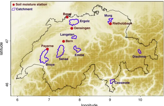
We use runoff measurements from several catchments located across Switzerland in different climate regimes to compare and to validate the models described above. Only a part of these runoff measurements can be used for validation whereas another part is used to calibrate the models. We additionally use soil moisture measurements from several stations near (some of) the considered catchments for a further, independent model validation. The loca-tions of the catchments and soil moisture staloca-tions are displayed in
Fig. 1, and their characteristics are listed inTables 2 and 3. Note
that the models are only applied in the catchments; whereas the streamflow validation is straightforward we use nearby soil
mois-ture stations for soil moismois-ture validation (seeTable 2). The
catch-ments are near-natural, i.e. the runoff is (almost) not impacted by human activity. From these catchments, we obtained daily stream-gauge measurements from 1987–2009 from the Swiss fed-eral office for the environment (FOEN).
The soil moisture data are provided by the SwissSMEX network (http://www.iac.ethz.ch/groups/seneviratne/research/SwissSMEX
[accessed on 7 March 2014], see alsoMittelbach and Seneviratne,
2012), the Rietholzbach research catchment (Seneviratne, 2012),
and a FOEN station at Oensingen. The measurements are taken in
different depths depending on the station (seeTable 2). For model
validation we derive an estimate of observed total-column soil moisture by adding the measurements from the different depths. We apply weights to each depth according to the vertical distance to the neighboring depths. This is necessary as there are usually more measurements in shallow depths as opposed to deeper depths. The weighting ensures a fair representation of low-level soil mois-ture dynamics in the total-column estimate. Since the soil moismois-ture measurements span different time periods depending on the station,
the site-specific soil moisture validations (Section 3.2) are
per-formed over different time periods. Note that in this validation we compare observed point-scale soil moisture with modeled soil
mois-ture from a respective nearby catchment (Table 2); mostly we chose
the catchment nearest to a particular soil moisture station, but we also ensured similar soil type and geology such that we compare measurements from Oensingen with model data from the Langeten catchment. A meaningful comparison despite the different scales is possible as we focus here on soil moisture dynamics (rather than the absolute values) which are representative for a larger area
surround-ing the measurement point (Mittelbach and Seneviratne, 2012).
Fur-thermore, we detrended soil moisture data from Rietholzbach and Berne to account for apparent linear drifts in the raw data. Note that the outlined shortcomings of the soil moisture data influence the results for all models in the same way, such that no particular model is favored. Further, the results at all stations are affected similarly, therefore no particular station is favored.
In order to run the models over the 1987–2012 time period (for which runoff and/or soil moisture data are available) we use grid-ded meteorological forcing data (http://www.meteosch weiz.ad-min.ch/web/en/services/data_portal/gridded_datasets.html [access ed on 7 March 2014]) from the Swiss federal office of meteorology and climatology (MeteoSwiss). Based on their dense network of meteorological stations they provide precipitation, temperature, global radiation and sunshine duration with a spatial resolution
of 2 km2 km. Additionally we use gridded observation-based
datasets of relative humidity and wind speed, which are also pro-vided by MeteoSwiss but in lower spatial resolution. To run the
longitude
latitude
6 7 8 9 10 46 47 Rietholzbach Oensingen Payerne Basel Bern Soil moisture stationCassarate Broye Sense Langeten Emme Ergolz Murg Dischma Catchment
Table 2
Overview of soil moisture stations. Note the corresponding catchments where the modeled soil moisture is computed.
Station Altitude (m) Location (lat/lon) Corresponding catchment Land cover Soil type Data period SM measure-ment depths (m) Basel 316 47.5°N 7.6°E Ergolz grassland silt loam 2009–2012 0.05, 0.1, 0.3, 0.5
Oensingen 450 47.3°N 7.7°E Langeten grassland silty clay loam 2002–2007 0.05, 0.1, 0.3, 0.5
Payerne 490 46.8°N 6.9°E Broye grassland loam 2008–2012 0.05, 0.1, 0.3, 0.5, 0.8
Berne 553 47.0°N 7.5°E Sense grassland loam 2009–2012 0.05, 0.1, 0.5, 0.8
Rietholz-bach 754 47.4°N 9.0°E Murg grassland loam 1994–2012 0.05, 0.15, 0.55, 0.8
Table 3
Overview of catchments and corresponding gauging stations. Catchment Mean altitude (m) Catchment area (km2
) Degree of glaciation (%) Mean temperature (°C) Gauging station Station coordinates
Ergolz 590 261 0 9.1 Liestal 47.5°N 7.7°E
Murg 650 79 0 8.3 Wängi 47.5°N 9.0°E
Broye 710 392 0 9.0 Payerne, Caserne D’aviation 46.8°N 6.9°E
Langeten 766 60 0 7.8 Huttwil, Häberenbad 47.1°N 7.8°E
Cassarate 990 74 0 9.0 Pregassona 46.0°N 9.0°E
Sense 1068 352 0 6.7 Thörishaus, Sensematt 46.9°N 7.4°E
Emme 1189 124 0 6.3 Eggiwil, Heidbüel 46.9°N 7.8°E
Dischma 2372 43 2.1 0.3 Davos, Kriegsmatte 46.8°N 9.9°E
Soil Moisture
Oensingen
dr
iest months
w
ettest months
dry intermediate wetRunoff [mm/d]
Langeten catchment
2002
2003
J F M A M J J A S O N D J F M A M J J A S O N D 13 5 1 0 1 5 Observations considered Observations not considered SWBMHBV PREVAH
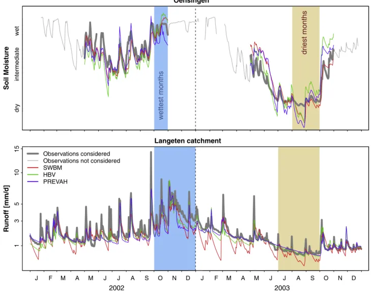
Fig. 2.Example time series for soil moisture and runoff at Oensingen and Langeten catchment, respectively. Gray lines indicated observations, colored lines represent model results. Modeled soil moisture time series are scaled to match the mean and standard deviation of the observations. Driest and wettest months are highlighted with brown and blue background, respectively. (For interpretation of the references to colour in this figure legend, the reader is referred to the web version of this article.)
models on catchment scale, we aggregated the data to the area of the considered catchments. Note that the different models use
dif-ferent forcing variables (seeTable 1).
In particular, the SWBM requires net radiation (Table 1)
whereas MeteoSwiss provides global radiation. To work around this problem we use measurements from the Rietholzbach site and we infer a relationship between net radiation on the one hand and global radiation and temperature on the other hand. For this purpose we perform a multi-linear least squares regression using 13 years of available data from the period 2000–2012. In total we compute 12 such regressions, one for each month as the underly-ing relationships change with season. We generally find high
frac-tions of explained net radiation variance (R20:9) supporting the
validity of this regression approach, except for the cold season
(R20:15). Then, however, net radiation is low anyway with
minor impacts on hydrology. The inferred relationships are then assumed to be valid throughout Switzerland and applied to esti-mate net radiation at the other sites considered in this study. This approach certainly introduces additional errors to the simple water balance simulations, but given the validation results presented in
Section4it is deemed successful.
3. Methodology
3.1. Calibration
In order to ensure a meaningful comparison of the models
described in Section 2we use the same data for calibration, i.e.
all models use identical runoff and meteorological forcing data
(see Section2.5). We use the first 10 years of runoff measurements
(1987–1996) to calibrate the models at each catchment and focus on the remaining years for validation. To reach an equilibrium model state to start our runs we use model-specific spin-up
peri-ods between 3 and 10 years (seeTable 1).
To determine the agreement between modeled and observed
runoff, all models use the Nash–Sutcliffe efficiency (Nash and
Sutcliffe, 1970; Schaefli and Gupta, 2007; hereafter referred to as
NSE) as (part of) the objective function that is maximized during
the calibration process (seeTable 1):
NSE¼1 P Q ObsiQSimi 2 P Q ObsiQObs 2 ð5Þ
whereQObsiis the observed daily runoff,QSimiis the corresponding
modeled daily runoff andQObsis the observed long-term mean
run-off. We apply(5)as objective function for SWBM and HBV. The
PRE-VAH model, however, uses an integrated objective function that comprises the NSE, the NSE with logarithmic values and a relative runoff error measure. This objective function was established in several earlier studies involving PREVAH; it allows us to evaluate this models in its characteristic configuration. Note that this slightly different objective function is a potential cause of differences in
model performance shown in Section4.
Using the HBV model we investigate this impact of different objective functions on the quality of the modeled soil moisture and runoff. For this purpose we calibrate the HBV model with a
slightly modified form of(5), additionally to the standard
configu-ration described above:
F¼NSE0:1
P
jQPObsiQSimij QObsi
ð6Þ where the combination of NSE with a volume error should counter-act the strong influence of outliers that arises from the squared
terms in Eq.(5).
For any model and any objective function the calibration may yield several parameter sets that perform almost equally well; the best is usually chosen to run the model. To further examine the impact of almost equally good but yet different parameter sets,
we additionally run the HBV model (using(5)as objective
func-tion) with 100 parameter sets instead of only the best, which yields 100 simulations of soil moisture and runoff at each considered site. The importance of the parameter uncertainty is then reflected in the difference of the performance of these 100 simulations.
3.2. Validation
We validate the models with respect to runoff and soil mois-ture. For runoff we focus on the time period 1997–2009 as this time period was not used in the calibration and the data can there-fore be regarded as independent. For soil moisture we focus on the time period with available measurements, which is different at
each station (seeTable 2). The soil moisture measurements allows
us to perform a truly independent comparison because this quan-tity is not used at all to calibrate the model parameters. Example time series of runoff and soil moisture along with corresponding
model output are displayed inFig. 2. We use the whole year to
per-form the validation in case of runoff, but for soil moisture we focus on the period May–October because measurements can be errone-ous in frozen soils and soil moisture dynamics are low in winter. Note that the runoff time of the river Langeten series actually ranges from 1997–2009, but we focus here on the 2002–2003 per-iod to enhance readability and because concomitant soil moisture observations from Oensingen are available.
As outlined in the introduction, the outcome of a model com-parison necessarily depends to some extent on the considered evaluation measure. To account for this and to compare different aspects of the agreement between models and observations, we employ several metrics:
Seasonal correlation: SC¼corðo;mÞ ð7Þ
Seasonal cor
Soil Moisture
Σ
2 2 2 1 1 3 3 3 3 2 1 1 1 2 3 8 14 8 PREV AH HBV SWBM Ranks at siteAnomal
y cor
2 2 2 1 1 3 3 3 3 3 1 1 1 2 2 8 15 7 PREV AH HBV SWBM Basel Oensingen Pa yern e Ber ne Rietholzb . increasing altitude 0.5 0.6 0.7 0.8 0.9 1.0 CorrelationFig. 3.Agreement between modeled and observed soil moisture, expressed as seasonal correlation and anomaly correlation. Refer to text for details. The models are ordered with respect to complexity (increasing from bottom to top), and the sites are ordered with respect to altitude (increasing from left to right). For each site and quantity ranks of the models are displayed, with the sum over all sites on the right side.
orefers to the observed time series andm denotes the corre-sponding modeled time series. This correlation is strongly influ-enced by the correspondence of observed and modeled seasonal cycles, especially in the case of soil moisture where the seasonal cycle is well pronounced.
Anomaly correlation:
AC¼corðo0;m0Þ ð8Þ
where
o0
n;y¼on;yon and mn0;y¼mn;ymn ð9Þ
The prime (0) denotes anomalies,nindicates the day of the year
andyis the year. For this measure, the seasonal cycle is removed
in both the observations and modeled time series before com-puting the correlation. The seasonal cycle is calculated as the mean yearly cycle over all years considered in the validation per-iod. Hence this metric reflects the ability of the models to cap-ture observed anomalies.
In the case of soil moisture we apply the Pearson correlation, whereas we use the Spearman rank correlation for runoff as it is more robust against outliers and thus better suited to deal with
the peaks shown in Fig. 2. The following three metrics are
com-puted in the runoff validation only, because they focus on the abso-lute values:
NSE: As in Eq.(5). The NSE represents the models’ ability to
esti-mate the absolute amount of water running off. It is sensitive to high flow periods (and to outliers) because of the squared differences.
NSE with logarithmic data: As in Eq.(5), but with logarithmic
time series of observations and model results. Compared to the common NSE this modified NSE has (i) an increased sensi-tivity to low flows, and (ii) is less impacted by extremely high values. This is because the logarithm increases differences between small values whereas it decreases differences between large values. This measure has been used in many previous
studies, e.g.Krause et al. (2005) and Zappa and Kan (2007).
Table 4
Summary of model ranks. Note that sometimes rank 1 is given to two models such that there is no rank 2.
SM HBV PREVAH Soil moisture All 1 3 1 Dry 1 3 2 Wet 3 2 1 Runoff All 3 1 1 Dry 1 1 1 Wet 3 1 1 Over-fitting 1 2 2
Seasonal cor
Validation
Σ
2 1 1 1 1 1 1 1 1 2 2 2 2 2 2 2 3 3 3 3 3 3 3 3 9 15 24 PREV AH HBV SWBMRanks at site
Anomal
y cor
3 2 2 1 2 2 1 1 1 1 1 2 1 1 2 2 2 3 3 3 3 3 3 3 14 11 23 PREV AH HBV SWBMNSE
PREV AH HBV SWBM 1 2 1 2 3 2 2 3 3 1 2 1 1 1 1 1 2 3 3 3 2 3 3 2 16 11 21NSE log
PREV AH HBV S WBM 2 1 2 1 1 1 2 1 1 2 1 2 2 2 1 2 3 3 3 3 3 3 3 3 11 13 24Ergolz Murg Broye
LangetenCassarateSenseEmmeDischma increasing altitude 0.5 0.6 0.7 0.8 0.9 1.0 Score / Correlation
Validation − Calibration
PREV AH HBV SWBMΣ
1 3 3 2 1 2 1 1 2 2 2 3 2 3 2 2 3 1 1 1 3 1 3 3 14 18 16 PREV AH HBV SWBM 2 3 3 3 2 3 1 1 3 2 2 2 3 1 2 2 1 1 1 1 1 2 3 3 18 17 13 PREV AH HBV SWBM 2 2 1 2 1 2 1 3 3 3 3 3 3 1 3 2 1 1 2 1 2 3 2 1 14 21 13 PREV AH HBV S WBM 2 3 3 3 1 3 1 2 3 2 2 2 2 2 3 1 1 1 1 1 3 1 2 3 18 17 13Ergolz Murg Broye
LangetenCassarateSenseEmmeDischma increasing altitude −0.2 −0.1 0.0 0.1 0.2 Difference
Fig. 4.Agreement between modeled and observed runoff, expressed as seasonal correlation, anomaly correlation and Nash–Sutcliffe efficiency. The results for the validation period 1997–2009 are displayed on the left side, the respective difference with results from the calibration period 1987–1996 is shown on the right side (validation minus calibration results). For each site and quantity ranks of the models are displayed, with the sum over all sites on the right side.
Comparing standard deviations: To further explore the agree-ment of the time variability between models and observations, we compute (i) the ratio between the standard deviations of the model output and respective observations, and (ii) the standard deviation of the time series of the differences obtained when subtracting the observations from the model results. Both
met-rics are displayed in a Taylor plot (see Section4.2). Whereas (i)
indicates the agreement of the seasonal cycle or of month-to-month variability between models and observations, (ii) rather captures the ability of the models to represent daily-weekly runoff anomalies.
To study the suitability of the models for extreme dry and wet conditions, we also compute the described metrics only taking into account the 5% driest and 5% wettest months, as determined from the observed runoff and soil moisture at each site, i.e. we do not necessarily consider the same time periods everywhere. The con-sidered time periods also vary in length, as the length of the inves-tigated time series vary (13 years for runoff, 4–19 years for soil moisture). The respective periods at Oensingen and in the Langeten
catchment are highlighted inFig. 2. Note that there are additional
months belonging to the 5% driest or 5% wettest months outside the displayed time period.
4. Results
In this section we present the results of the validation of the models with soil moisture and runoff observations. Furthermore we investigate the models’ performance during extreme condi-tions, i.e. drought and flood periods. To address the question whether model performance improves with complexity, we com-pare the models with each other throughout this section by rank-ing their performance at each site. The sum of the ranks of a particular model computed over all sites is then a measure for (rel-ative) model performance.
4.1. Soil moisture validation
As mentioned in Section2.5, the soil moisture measurements
considered in this study allow us to perform a truly independent validation of the models because this quantity is not used for model training. Due to the lack of soil moisture measurements
such a validation (Schlosser et al., 2000; Gurtz et al., 2003) is rare
and may therefore provide new insights. The results are displayed
inFig. 3, with color-coded seasonal correlation and anomaly
corre-lation values for each model at each site. Note the different consid-ered time periods and measurement depths at the respective sites
(Table 2). Sites are ordered with respect to altitude, starting on the
left with the lowest station (Basel). Moreover, the models are ordered according to their complexity, starting with the most sim-ple model on top. As described above, a model ranking is computed at each of the stations, and the sum of all ranks is displayed on the right.
Generally we find decreasing model performance with increas-ing altitude. But even at the highest site (Rietholzbach) the models agree with the observations to some extent, as the color scale starts at 0.5. The colors patterns for the results of the seasonal correla-tions and the anomaly correlacorrela-tions are similar. This suggests that the models’ ability to capture the seasonal cycle is linked with the ability to represent (daily-weekly) anomalies. As indicated by the ranking sums displayed on the right the SWBM and PREVAH clearly outperform the HBV model in the case of soil moisture. This result is noteworthy since it indicates that complex models such as HBV do not necessarily outperform parsimonious models such as the SWBM. It seems that the complexity of HBV is inadequate to
make optimal use of the input data in order to resemble observed soil moisture dynamics. This structural problem leads to an
over-parametrization (Perrin et al., 2001), i.e. the model parameters
cap-ture random noise besides the underlying hydrological processes impacting soil moisture. Comparing the SWBM and PREVAH, the first model seems to be better suited at low altitudes whereas
Standard deviation Standard deviation 0.00.0 0.5 1.0 1.5 0.5 1.0 1.5 0.5 1 1.5 0.1 0.2 0.3 0.4 0.5 0.6 0.7 0.8 0.9 0.95 0.99 Correlation
SWBM
OBS Standard deviation Standard deviation 0.00.0 0.5 1.0 1.5 0 .5 1.0 1.5 0.5 1 1.5 0.1 0.2 0.3 0.4 0.5 0.6 0.7 0.8 0.9 0.95 0.99 CorrelationHBV
OBS Standard deviation Standard deviation 0.00.0 0.5 1.0 1.5 0 .5 1.0 1 .5 0.5 1 1.5 0.1 0.2 0.3 0.4 0.5 0.6 0.7 0.8 0.9 0.95 0.99 CorrelationPREV
AH
OBS Ergolz Murg Broye Langeten Cassarate Sense Emme Dischma Calibration 1987−1996 Validation 1997−2009Fig. 5.Taylor plots for runoff evaluation. Colors refer to respective catchments. The results are shown for calibration (circles) and validation period (dots), respectively. Note that a model that perfectly agrees with observations would fall on point ’OBS’. (For interpretation of the references to colour in this figure legend, the reader is referred to the web version of this article.)
the latter one performs slightly better at Berne and Rietholzbach, leading to an overall similar performance of the two models across all considered sites.
An overall ranking of the models in terms of soil moisture is
provided inTable 4. As described in Section2.4, PREVAH is based
on HBV but it employs soil information with higher spatial resolu-tion. These modifications are deemed successful predominantly in mountainous regions as PREVAH outperforms HBV especially in higher altitudes in the case of soil moisture.
4.2. Runoff validation
The runoff validation is performed with independent measure-ments, as we divided the time period with available observations into a calibration period (1987–1996) where measurements are used for model training, and a validation period (1997–2009) where measurements are used exclusively to assess the models’
performance. The results are displayed on the left side inFig. 4.
The order of the models and of the catchments follows the same
criteria as inFig. 3, also the color scale is the same. As described
in Section 3.2 we compare not only the runoff dynamics (i.e.
changes over time) between models and observations as in the case of soil moisture, but also the absolute runoff amounts using the NSE. Note that in order to compute NSElog scores for the runoff simulated by the SWBM we added 0.3 mm/d for every day and every catchment, because the raw simulated runoff decreased to zero occasionally, leading to infinite NSElog values, whereas we find minimum runoff amounts of around 0.3 mm/d for the other models.
As inFig. 3, we find a tendency towards weaker model
perfor-mance in higher altitude catchments, but less pronounced than for soil moisture. Comparing the seasonal and anomaly
correla-tions with the soil moisture results inFig. 3reveals a slightly better
ability of the models to simulate runoff dynamics. This difference may be partly due to the shortcomings of the soil moisture
valida-tion discussed in Secvalida-tion2.5, or could also be affected by the fact
that the models were calibrated with runoff measurements. The sums of the ranks are highest for the SWBM for all considered met-rics which means that it does not simulate runoff as well as the
other models, despite its good soil moisture performance. HBV and PREVAH perform better; their relative performance depends on the considered evaluation metric (i.e. on the considered charac-teristics of the modeled runoff). Across the sites considered in this study, HBV outperforms PREVAH in terms of high flows (NSE) and also for anomalies (anomaly correlation). In contrast, PREVAH agrees clearly better with observations for seasonality (seasonal correlation) and slightly better for low flows (NSElog). Unlike in the soil moisture validation results the ranking of the models dif-fers with respect to the considered runoff characteristic and hence with regard to the evaluation metric. For a comprehensive assess-ment of model performance different metrics need to be consid-ered as each compares certain aspects of the modeled and
observed time series (see Section3.2). Also in contrast to the soil
moisture validation results the complexity of HBV and PREVAH is adequate to capture streamflow dynamics whereas the SWBM misses the underlying processes. This result indicates that different aspects of the hydrological system may require different complex-ity in the corresponding parts of the models.
On the right inFig. 4we illustrate the changes of the models’
performance between calibration and validation period. As expected, the agreement between models and observations is gen-erally weaker during the validation period across all considered metrics, apart from some exceptions. Even if there seems to be no trend with respect to catchment altitude, large differences are found for the alpine Dischma catchment, but only in terms of the anomaly correlation and the NSE. The reason for this feature is the poor agreement of models and measurements in 2001. Although the seasonal cycle with high runoff values from April through November and low values during the cold season is gener-ally captured, there is significant disagreement between the model and observations from April until September. In all other years the models are performing much better in this catchment, therefore we speculate that some event (such as a mountain slide) may have altered the natural runoff dynamics for some months in 2001. Overall the smallest decreases of the considered correlations and scores are found for the SWBM, indicating a comparatively strong temporal consistency of its performance. Only in terms of the sea-sonal correlation, the PREVAH model is more consistent. At the
Anomaly correlation
Soil moisture
Σ
2 3 2 2 1 3 2 3 3 2 1 1 1 1 3 10 13 7 PREV AH HBV SWBMRanks at site
wettest months 1 1 2 3 1 2 2 1 2 3 3 3 3 1 2 8 10 12 PREV AH HBV SWBM BaselOensingen Payerne Berne Rietholzb.
increasing altitude
Runoff
Σ
3 2 2 3 2 1 2 2 2 3 1 2 1 3 1 2 1 1 3 1 3 2 3 2 17 15 16 3 2 1 2 3 2 1 1 1 3 2 1 1 1 2 2 2 1 3 3 2 3 3 3 15 13 20Ergolz Murg BroyeLangeten
CassarateSenseEmmeDischma increasing altitude 0.0 0.2 0.4 0.6 0.8 1.0 Correlation driest months
Fig. 6.Anomaly correlation for soil moisture and runoff under extreme conditions. Computed from either the 5% driest (upper row) or 5% wettest months (lower row). Order of models and sites as inFigs. 3 and 4; also ranks are computed in the same way.
same time PREVAH shows the largest differences in terms of two out of the four considered metrics (anomaly correlation and NSE-log), which is probably due to over-fitting in this model (i.e. the model parameters depend not only on the natural runoff variations during the calibration period but also to some extent on random noise). We find the largest differences for the two remaining met-rics for the HBV model simulations, together with the sums of ranks that are close to the highest (PREVAH) for the other two met-rics. In summary, these results suggests that the over-fitting prob-lem diagnosed from the data investigated here is most pronounced for HBV, and also of relevance for the PREVAH model, whereas it seems to be less important for the SWBM. This finding matches with the lower number of model parameters in the SWBM as
com-pared to the other two models (seeTable 1). However, at the same
time the lower number of parameters obviously limits the ability to resemble observed runoff dynamics as indicated by the compar-atively weak performance of the SWBM. This underlines the importance of an adequate complexity of a model (and parts thereof); if a model is overly complex it may suffer from over-parametrization and if it is too simple it may suffer from an incom-plete representation of relevant processes.
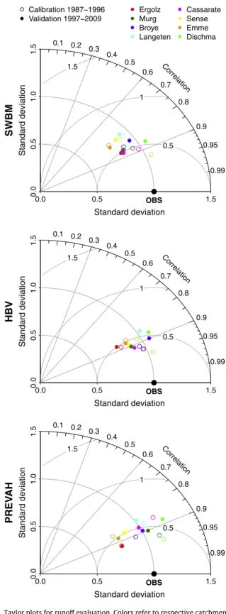
For a more complete assessment of the models performance we employ Taylor plots which integrate several (additional)
evalua-tion metrics (Secevalua-tion3.2).Fig. 5displays Taylor plots for all models
containing all investigated sites. As introduced in Section3.2, the
radial distance from the origin represents the relative standard deviation of the modeled runoff with respect to corresponding observations. A perfect model would be located on the 1.0-circle. The distance to the point labeled ’OBS’ indicates the standard devi-ation of the difference between modeled and observed runoff, a perfect model would be located at point ’OBS’. As expected, the points representing the calibration period are usually located clo-ser to ’OBS’ and the 1.0-circle. The difference between calibration and validation results is rather small compared to the differences we find across the investigated catchments. The Taylor plots reveal that the SWBM underestimates the runoff variability at most sites, that HBV also has a slight tendency towards such an underestima-tion, whereas PREVAH has no obvious tendency in any direction. The variability of the differences between simulated and observed runoff is generally the largest for the SWBM and the smallest for HBV. Overall these findings compare well with the results of
Fig. 4. A summary ranking of the models’ runoff performance is
provided inTable 4.
4.3. Validation of dry and wet extremes
Whereas the previous sections focused on the ability of the models to simulate soil moisture and runoff during any conditions, we investigate here their performance during extreme events. This is especially important as the performance of a model may differ in extreme conditions as opposed to average conditions. Furthermore information on model performance during floods or droughts is relevant for decision making based on model predictions. To inves-tigate hydrological extremes, we focus on the 5% driest and 5%
wettest months, respectively, as described in Section3.2.
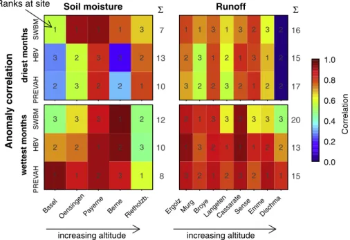
Fig. 6presents the results in terms of the anomaly correlation.
This metric is suited for the relatively short time periods consid-ered here and it can be computed for both soil moisture and runoff. Comparing the results in this figure with corresponding anomaly
correlations inFigs. 3 and 4shows that the models’ performance
is degraded with respect to observations in the case of extreme events (note the different color scales). The models’ performance seems to be overall higher in the case of wet events in contrast to dry extremes. Furthermore there is no apparent trend with respect to altitude. Whereas the general performance in simulating
soil moisture was similar for the SWBM and PREVAH in Section4.1,
we find in the case of extremes that the SWBM performs better for dry anomalies and PREVAH seems to be rather suitable for wet
anomalies. As in Section4.1, HBV shows a weak performance in
simulating soil moisture, especially during dry conditions, and with slightly better agreement with observations during wet con-ditions. In contrast to this, HBV slightly outperforms the other models in simulating runoff extremes. As for the soil moisture extremes, HBV and PREVAH perform better during wet anomalies
Standard deviation Standard deviation 0.00.0 0.5 1.0 1.5 0.5 1.0 1.5 0.5 1 1.5 0.1 0.2 0.3 0.4 0.5 0.6 0.7 0.8 0.9 0.95 0.99 Correlation
SWBM
OBS W WW W W W W W D D D D D D D D Standard deviation Standard deviation 0.00.0 0.5 1.0 1.5 0 .5 1.0 1.5 0.5 1 1.5 0.1 0.2 0.3 0.4 0.5 0.6 0.7 0.8 0.9 0.95 0.99 CorrelationHBV
OBS W W W W W W W W D D D D D D D Standard deviation Standard deviation 0.00.0 0.5 1.0 1.5 0 .5 1.0 1 .5 0.5 1 1.5 0.1 0.2 0.3 0.4 0.5 0.6 0.7 0.8 0.9 0.95 0.99 CorrelationPREV
AH
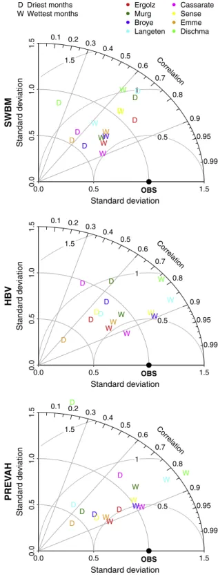
OBS W W W W W W W W D D D D D D D D Ergolz Murg Broye Langeten Cassarate Sense Emme Dischma D W Driest months Wettest monthsFig. 7.Same as inFig. 5, but focusing on extreme conditions, i.e. the 5% driest months (denoted with ‘D’) and 5% wettest months (denoted with ‘W’).
as compared to dry events, whereas we find the opposite for the SWBM. Despite its comparatively weak runoff performance in
Fig. 4, it simulates dry anomalies as well as the other models. These
results illustrate the dependency of (relative) model performance on the conditions. For a complete validation it is necessary to com-pare a model with observations under different (wetness) condi-tions to assess its strengths and weaknesses. These information can then also be used to improve the model through the inclusion of particular processes or the simplification of specific modules.
InFig. 2it seems that the SWBM has difficulties to simulate the
runoff at the Langeten catchment during dry periods. This
impres-sion is confirmed inFig. 4 through the low NSElog score of the
SWBM, which reflects the models ability to simulate low flows. However, the anomaly correlation for the SWBM during dry
extremes displayed inFig. 6 is comparatively high. What seems
to be a contradiction at the first glance is actually a nice example on why it is necessary to distinguish between the absolute values
and dynamics when validating a model.Fig. 2shows indeed a bias
of the SWBM, which is actually exaggerated through the logarith-mic scale in the figure. But it also shows that the model captures the observed runoff variability comparatively well during dry con-ditions, whereas PREVAH for instance simulates almost no day-to-day variability during the highlighted dry period in summer 2003. We furthermore investigated the extreme runoff events in
terms of Taylor plots which are presented inFig. 7. Compared to
Fig. 5the points representing both extremes are further away from
the ’OBS’ point and also from the 1.0-circle, indicating degraded model performance for simulating extreme runoff events in terms of absolute values. This is in line with the anomaly correlation results described above. Focusing on the dry events we find a
similar performance of the models in terms of the standard devia-tion of the difference time series (observadevia-tions minus model simu-lations). Furthermore there is a general underestimation of variability as compared with observations (most ’D’ points are within the 1.0-circle), although less pronounced in the case of the SWBM. In contrast, this model underestimates the variability for wet extremes, whereas the other models compare better with observations in this respect. The overall performance during wet extremes is better than during dry events, again confirming the
results obtained with the anomaly correlation metric.Table 4
sum-marizes the model performances during extreme events.
4.4. Differences between models
Although the governing equations of the models we consider are similar, we find relatively large differences between their per-formance as discussed in the previous sub-sections. Such differ-ences in the performance of the models may arise from (i) the different objective functions of the models, (ii) uncertainty of the calibrated parameters (equifinality, i.e. several parameter sets may perform similarly well in the calibration), (iii) different mete-orological forcing variables and/or (iv) the use of different methods to estimate evaporation. Regarding the fourth point, the main dif-ference is the use of long-term mean values for potential evapora-tion as input for HBV, whereas time series of radiaevapora-tion were used in the other two models. The results indicate that the latter approach is better suited to simulate interannual variablilities.
To study the impact of the first two causes we use the HBV model calibrated with different objective functions and run with the 100 best performing parameter sets from the model
calibra-comparison vs multi−model mean
comparison vs obs
SWBM
PREV
AH
HBV
HBV with diff HBV with
. calibr . diff . par am. Seasonal correlation
Soil Moisture
Mean cor across all sites
SWBM
PREV
A
H
HBV
HBV with diff HBV with
. calibr . diff . par am. Anomaly correlation Dr y We t SWBM PREV AH HBV
HBV with diff HBV with
. calibr
.
diff
. par
am.
Anomaly cor, Extremes NSE
0.4 0.5 0.6 0.7 0.8 0.9 1 0.4 0.5 0.6 0.7 0.8 0.9 1 0.4 0.5 0.6 0.7 0.8 0.9 1 0.4 0 .5 0.6 0 .7 0.8 0 .9 1 0.4 0.5 0.6 0.7 0.8 0.9 1 0.4 0 .5 0.6 0 .7 0.8 0 .9 1 0.4 0 .5 0.6 0 .7 0.8 0 .9 1 SWBM PREV AH HBV
HBV with diff HBV with
. calibr . diff . par a m.
Runoff
Mean cor across all sites
SWBM
PREV
AH
HBV
HBV with diff HBV with
. calibr . diff . par a m. Dr y We t SWBM PREV AH HBV
HBV with diff HBV with
. calibr . diff . par a m. SWBM PREV AH HBV
HBV with diff HBV with
. calibr . diff . par a m.
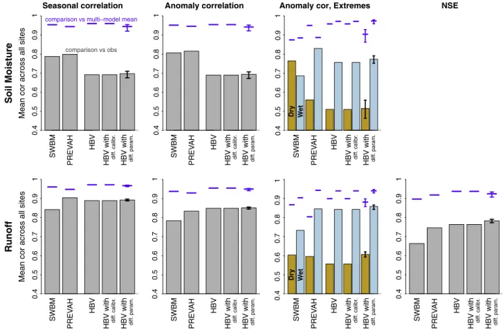
Fig. 8.Summary ofFigs. 3, 4 and 6. Furthermore respective results are included for the HBV model with different objective function and with 100 similarly well performing parameter sets. For the different parameter sets the performance of the ensemble mean is shown along with whiskers that denote the 95% and 5% quantile. Blue lines indicate the corresponding model results assessed against a multi-model mean instead of observations. (For interpretation of the references to colour in this figure legend, the reader is referred to the web version of this article.)
tion, as described in Section3.1. The results are displayed inFig. 8
along with a summary ofFigs. 3, 4 and 6. The impact of the
objec-tive function and of the parameter uncertainty on the performance of HBV is generally low. The model performs very similar with respect to observations despite different objective functions used in the calibration, also the spread between the performance of the different parameter sets is small compared to the difference between HBV and the other models. Only when focusing on extreme events the role of the objective function and the parame-ter uncertainty is slightly more important, especially for dry extremes. For the sites considered in this study we can conclude that except for dry extremes the choice of the model is more important for the quality of the modeled soil moisture and runoff compared to the objective function or the parameter uncertainty. Note, however, that the different objective functions employed for HBV were rather similar, and thus that more different objective functions may lead to larger differences in the model results.
Moreover we investigated the relative importance of the inter-model differences versus the difference between inter-models and respective observations. For this purpose we replaced the observa-tions with a multi-model mean; we find generally clearly better model performance when using the multi-model mean as
refer-ence (blue lines in Fig. 8). This indicates that the differences
between the models are small compared to the differences with respect to observations, in terms of both soil moisture and runoff under normal and extreme conditions. This finding is in line with
the structural similarities of the models.Fig. 8 also shows that
the models all compare similarly well to the multi-model mean, indicating that none of the considered models is an outlier. Inter-estingly, the models agree better with respect to wet extremes than for dry extremes.
5. Conclusions
In this study we evaluated and compared three hydrological models with observations of runoff and soil moisture from multi-ple sites across Switzerland. We chose models of different com-plexity to investigate whether the comcom-plexity level influences their performance. With available soil moisture measurements we could perform a novel, truly independent validation of the models because this quantity is not used at all for model training. To ensure comparability across the models, the catchment-specific calibration was done with the same data and similar objective functions for all models.
Answering the question posed in the title, the results of our case study support only partly the hypothesis that more sophisticated models outperform simple models. For runoff the more complex models PREVAH and HBV outperform the simple water balance model, but for soil moisture the SWBM has overall a similar perfor-mance as PREVAH and clearly better than HBV. Comparing the most complex model PREVAH with the HBV model on which it is based we find better performance only in the case of soil moisture simulation. During extreme dry events the SWBM performs gener-ally better whereas its performance is degraded in extremely wet conditions. For the other two models we find the opposite behav-ior. They therefore seem to be suited for flood prediction whereas the SWBM fits better during droughts. These findings indicate that model performance varies with respect to the hydrological condi-tions. Hence it is advisable for future validation studies to sepa-rately focus on the hydrological extremes as also the model predictions in such situations are especially important for decision makers. All models agree slightly better with observations from low altitude sites compared with those at high altitudes. A possible reason is that the models have difficulties in capturing the pro-cesses related to snow and ice; additionally the soil moisture,
runoff and precipitation measurements may be more uncertain in high altitudes. Comparing the performances of the models dur-ing the calibration and the validation period in the case of runoff we found larger decreases for HBV and PREVAH. This seems to be a consequence from higher number of parameters as compared to the SWBM which may lead to over-fitting, i.e. the model param-eters are impacted by random noise besides the natural runoff variations. Our study illustrates that adequate complexity of a model (and even particular processes simulated therein) is impor-tant; if models are overly complex such as HBV in the case of soil moisture modeling they suffer from over-parametrization but if they are too simple they miss relevant processes such as the SWBM in the case of runoff.
We note that the results differ with respect to the considered site and conditions, and depend therefore on the investigated sites and time frames. We used different metrics to assess the agree-ment between models and observations, analyzing the temporal dynamics on short and long time scales and in the case of runoff also the absolute offset with a focus on low and high flows. Inter-estingly, the results were rather similar independently of the met-ric considered, especially in the case of soil moisture.
The governing equations of the models are almost the same except for different scaling of ET (potential ET vs. net radiation). Applying the HBV model in different configurations we find that model results are rather insensitive to the different objective func-tions and uncertainty of the calibrated parameters. Therefore the performance differences we report may be due to the different ET scaling or different meteorological forcing variables (only pre-cipitation and temperature are used by all models).
We assessed the (relative) performance of the models under dif-ferent conditions, with difdif-ferent evaluation metrics and in terms of different quantities. This multi-dimensional approach allowed to identify potential strengths and weaknesses of the models such as the soil moisture dynamics in the SWBM under dry conditions or PREVAH’s simulated runoff under dry conditions, respectively. These results may also help to efficiently improve the models in the future by addressing their specific weaknesses. We find that added complexity does not necessarily lead to improved perfor-mance of hydrological models, and that perforperfor-mance can vary greatly depending on the considered hydrological variable (e.g. runoff vs. soil moisture) or hydrological conditions (floods vs. droughts).
Acknowledgments
We thank Heidi Mittelbach (SwissSMEX network, http://www.ia-c.ethz.ch/groups/seneviratne/research/SwissSMEX [accessed on 7 March 2014]) and Christof Ammann for providing the soil moisture data. Moreover, we acknowledge the Swiss federal office for the envi-ronment (FOEN) for sharing runoff data and the Swiss federal office of meteorology and climatology (MeteoSwiss) for sharing gridded meteorological forcing data (http://www.meteoschweiz.admin.ch/ web/en/services/data_portal/gridded_datasets.html [accessed on 7 March 2014]).
We acknowledge financial support by the Swiss National Foun-dation through the NRP61 DROUGHT-CH project, and partial sup-port from the EU-FP7 DROUGHT-R&SPI project.
References
Andreassian, V. et al., 2009. Crash tests for a standardized evaluation of hydrological
models. Hydrol. Earth Syst. Sci. 13, 1757–1764.
Bergström, S., 1976. Development and application of a conceptual runoff model for Scandinavian catchments. SMHI Report, RHO 7.
Bergström, S., 1995. The HBV model. Computer models of watershed hydrology, pp. 443–476.
Beven, K., 1989. Changing ideas in hydrology – the case of physically-based models.
J. Hydrol. 105 (1–2), 157–172.
Bosshard, T., Carambia, M., Goergen, K., Kotlarski, S., Krahe, P., Zappa, M., SchSr, C., 2013. Quantifying uncertainty sources in an ensemble of hydrological
climate-impact projections. Water Resour. Res. 49 (3), 1523–1536.
Budyko, M.I., 1974. Climate and Life. Academic Press.
Donohue, R.J., Roderick, M.L., McVicar, T.R., 2007. On the importance of including vegetation dynamics in Budyko’s hydrological model. Hydrol. Earth Syst. Sci. 11
(2), 983–995.
Gent, P.R. et al., 2011. The community climate system model version 4. J. Climate 24
(19), 4973–4991.
Gurtz, J., Baltensweiler, A., Lang, H., 1999. Spatially distributed hydrotope-based modelling of evapotranspiration and runoff in mountainous basins. Hydrol.
Processes 13, 2751–2768.
Gurtz, J., Zappa, M., Jasper, K., Lang, H., Verbunt, M., Badoux, A., Vitvar, T., 2003. A comparative study in modeling runoff and its components in two mountainous
catchments. Hydrol. Processes 17 (2), 297–311.
Holländer, H.M. et al., 2009. Comparative predictions of discharge from an artificial catchment (Chicken Creek) using sparse data. Hydrol. Earth Syst. Sci. 13, 2069–
2094.
IPCC, 2013. The physical science basis. <https://www.ipcc.ch/report/ar5/wg1/> Kirchner, J., 2009. Catchments as simple dynamical systems: catchment
characterization, rainfall-runoff modeling, and doing hydrology backward.
Water Resour. Res. 45 (W02), 429.
Kobierska, F., Jonas, T., Zappa, M., Bavay, M., Magnusson, J., Bernasconi, S.M., 2013. Future runoff from a partly glacierized watershed in Central Switzerland: a 2
model approach. Adv. Water Res. 55, 204–214.
Koboltschnig, G.R., Schoener, W., Holzmann, H., Zappa, M., 2009. Contribution of glacier melt to stream runoff under extreme climate conditions in the summer
of 2003. Hydrol. Processes 23, 1010–1018.
Koster, R.D., Mahanama, S., 2012. Land surface controls on hydroclimatic means and
variability. J. Hydrometeorol. 13, 1604–1620.
Krause, P., Boyle, D.P., Bäse, F., 2005. Comparison of different efficiency criteria for
hydrological model assessment. Adv. Geosci. 5, 89–97.
Lindström, G., Johansson, B., Persson, M., Gardelin, M., Bergström, S., 1997. Development and test of the distributed HBV-96 hydrological model. J.
Hydrol. 201, 272–288.
Mittelbach, H., Seneviratne, S.I., 2012. A new perspective on the spatio-temporal variability of soil moisture: temporal dynamics versus time invariant
contributions. Hydrol. Earth Syst. Sci. 16, 2169–2179.
Nash, J.E., Sutcliffe, J.V., 1970. River flow forecasting through conceptual models
part I – a discussion of principles. J. Hydrol. 10 (3), 282–290.
Orth, R., Seneviratne, S.I., 2013a. Propagation of soil moisture memory to streamflow and evapotranspiration. Hydrol. Earth Syst. Sci. 17, 3895–3911.
http://dx.doi.org/10.5194/hess-17-3895-2013.
Orth, R., Seneviratne, S.I., 2013b. Predictability of soil moisture and streamflow on sub-seasonal timescales: a case study. J. Geophys. Res. 118 (19), 10.963–10.979.
http://dx.doi.org/10.1002/jgrd.50846.
Orth, R., Koster, R.D., Seneviratne, S.I., 2013. Inferring soil moisture memory from streamflow observations. J. Hydrometeorol. 14, 1773–1790.http://dx.doi.org/
10.1175/JHM-D-12-099.1.
Perrin, C., Michel, C., Andreassian, V., 2001. Does a large number of parameters enhance model performance? Comparative assessment of common catchment
model structures on 429 catchments. J. Hydrol. 242 (3–4), 275–301.
Perrin, C., Dilks, C., Barlund, I., Payan, J.L., Andreassian, V., 2006. Use of simple rainfall-runoff models as a baseline for the benchmarking of the hydrological component of complex catchment models. Archiv. Hydrobiol. Large Rivers
Suppl. 17 (102), 75–96.
Press, W.H., Teukolsky, S.A., Vetterling, W.T., Flannery, B.P., 1992. Numerical Recipes in FORTRAN: The Art of Scientific Computing. Cambridge University Press, pp.
617–620.
Schaefli, B., Gupta, H.V., 2007. Do Nash values have value? Hydrol. Processes 21
(15), 2075–2080.
Schattan, P., Zappa, M., Lischke, H., Bernhard, L., Thnrig, E., Diekkrnger, B., 2013. An approach for transient consideration of forest change in hydrological impact studies. Climate and Land Surface Changes in Hydrology, Proceedings of H01, IAHS-IAPSO-IASPEI Assembly, IAHS Publ. 359, pp. 311–319.
Schlosser, C.A., Slater, A.G., robock, A., Vinnikov, A.J.P.K.Y., Henderson-Sellers, A., Speranskaya, N.A., Mitchell, K., 2000. Simulations of a boreal grassland hydrology at Valdai, Russia: PILPS Phase 2(d). Monthly Weather Rev. 128,
301–321.
Seibert, J., 1999. Regionalisation of parameters for a conceptual rainfall-runoff
model. Agric. Forest Meteorol. 98, 279–293.
Seibert, J., Vis, M., 2012. Teaching hydrological modeling with a user-friendly catchment-runoff-model software package. Hydrol. Earth Syst. Sci. 16, 3315–
3325.
Seneviratne, S.I. et al., 2012. The Rietholzbach research site: analysis of 32-year hydroclimatological time series and 2003 drought at a Swiss pre-alpine
catchment. Water Resour. Res. 48 (W06), 526.
Viviroli, D., Zappa, M., Gurtz, J., Weingartner, R., 2009. An introduction to the hydrological modelling system PREVAH and its pre- and post-processing-tools.
Environ. Modell. Softw. 24, 1209–1222.
Viviroli, D., Zappa, M., Schwanbeck, J., Gurtz, J., Weingartner, R., 2009. Continuous simulation for flood estimation in ungauged mesoscale catchments of Switzerland – Part I: modelling framework and calibration results. J. Hydrol.
377, 191–207.
Viviroli, D., Mittelbach, H., Gurtz, J., Weingartner, R., 2009. Continuous simulation for flood estimation in ungauged mesoscale catchments of Switzerland – Part II:
parameter regionalization and flood estimation results. J. Hydrol. 377, 208–225.
Zappa, M., 2008. Objective quantitative spatial verification of distributed snow cover simulations – an experiment for entire Switzerland. Hydrol. Sci. J. 53 (1),
179–191.
Zappa, M., Gurtz, J., 2003. Simulation of soil moisture and evapotranspiration in a soil profile during the 1999 MAP-Riviera Campaign. Hydrol. Earth Syst. Sci. 7,
903–919.
Zappa, M., Kan, C., 2007. Extreme heat and runoff extremes in the Swiss Alps. Nat.
Hazards Earth Syst. Sci. 7, 375–389.
Zappa, M., Pos, F., Strasser, U., Warmerdam, P., Gurtz, J., 2003. Seasonal water balance of an Alpine catchment as evaluated by different methods for spatially
distributed snowmelt modelling. Nord Hydrol. 34 (3), 179–202.
Zappa, M., Bernhard, L., Fundel, F., Jörg-Hess, S., 2012. Vorhersage und Szenarien von Schnee- und Wasserressourcen im Alpenraum. Forum fnr Wissen, pp. 19–27.