Open PRAIRIE: Open Public Research Access Institutional
Repository and Information Exchange
Electronic Theses and Dissertations
2018
A Scale Space Local Binary Pattern (SSLBP) –
Based Feature Extraction Framework to Detect
Bones from Knee MRI Scans
Jinyeong Mun
South Dakota State University
Follow this and additional works at:https://openprairie.sdstate.edu/etd
Part of theBiomedical Commons,Computer Engineering Commons, and theMedical Biotechnology Commons
This Thesis - Open Access is brought to you for free and open access by Open PRAIRIE: Open Public Research Access Institutional Repository and Information Exchange. It has been accepted for inclusion in Electronic Theses and Dissertations by an authorized administrator of Open PRAIRIE: Open Public Research Access Institutional Repository and Information Exchange. For more information, please [email protected]. Recommended Citation
Mun, Jinyeong, "A Scale Space Local Binary Pattern (SSLBP) – Based Feature Extraction Framework to Detect Bones from Knee MRI Scans" (2018).Electronic Theses and Dissertations. 2951.
EXTRACTION FRAMEWORK TO DETECT BONES FROM KNEE MRI SCANS
BY
JIN YEONG MUN
A thesis submitted in partial fulfilment of the requirements for the Master of Science
Major in Computer Science South Dakota State University
ACKNOWLEDGMENTS
I would like to express my special thanks of gratitude to my advisor, Prof. Sung Shin, who helped me in doing a lot of research and supported me to study and work in this field of Computer Science, as well as my thesis committee, Prof. Alireza Salehnia, Prof. Kwanghee Won, and Prof. Marie-Pierre Baggett for their time and intellectual contributions.
This work was supported by Electronics and Telecommunications Research Institute (ETRI) grant funded by the Korean government [18ZR1230, Research on Beam Focusing Algorithm for Microwave Treatment]. I appreciate their support for helping me to finish this work successfully.
Finally, I would like to extend my deepest gratitude to my family for not only their support but also for all they have done to enable my achievements.
TABLE OF CONTENTS
ABBREVIATIONS ... vi
LIST OF FIGURES ... vii
LIST OF TABLES ... viii
ABSTRACT ... ix 1. INTRODUCTION ... 1 2. LITERATURE REVIEW ... 4 3. RELATED WORK ... 6 4. PROPOSED MODEL ... 8 4.1 TRAINING PHASE ... 9
4.1.1 Cropped Training Data ... 9
4.1.2 Feature Extraction ... 9
4.1.3 Training with SVM ... 12
4.2 SEGMENTATION PHASE ... 13
4.2.1 Pre-Processing ... 13
4.2.2 Feature Extraction & Classification ... 14
4.2.3 Post-Processing ... 15
5. EXPERIMENTAL RESULTS AND ANALYSIS ... 16
6. CONCLUSIONS ... 24
ABBREVIATIONS
ACC Accuracy
CNN Convolutional Neural Networks
DNN Deep Neural Networks
FCM Fuzzy C-means Clustering
MCC Matthews Correlation Coefficient
MRI Magnetic Resonance Imaging
OA Osteoarthritis
ROI Region of Interest
LIST OF FIGURES
Figure 1: Diagram of proposed methodology ... 2
Figure 2: An example of two classes with vectors ... 4
Figure 3: An example of basic concept of Support Vector Machine with found hyperlane ... 5
Figure 4: Proposed Method of Segmentation Pipeline ... 8
Figure 5: Example cropped images of bone parts other parts. ... 9
Figure 6: Set up the window size for feature extraction ... 10
Figure 7: Feature Vector description ... 11
Figure 8: The result image of pre-processing step ... 13
Figure 9: The result of SVM classification with SSLBP feature extraction ... 14
Figure 10: The result images ... 15
Figure 11: Comparison of the proposed method with two existing method ... 18
Figure 12: Comparison of Training Accuracy, ACC and MCC evaluation ... 20
Figure 13: The result comparison images with difference size of training dataset ... 22
Figure 14: The result images for comparison with the ground truth images, the result of fuzzy c-means methodology, the result of deep feature extraction, and the result of proposed methodology. ... 23
LIST OF TABLES
TABLE 1: Definition of each category for comparison ... 17 TABLE 2: Average percentage of each category ... 18 TABLE 3: Results of ACC and MCC evaluation ... 18 TABLE 4: Average percentage of each category for two different size of trained data .. 19 TABLE 5: Results of Training Accuracy, ACC and MCC evaluation for two different size of trained data ... 20 TABLE 6: Results of Training Accuracy for two different size of cropped image ... 21 TABLE 7: Results of Training Accuracy for two different size of cropped image ... 21
ABSTRACT
A SCALE SPACE LOCAL BINARY PATTERN (SSLBP) - BASED FEATURE EXTRACTION FRAMEWORK TO DETECT BONES FROM KNEE MRI SCANS
JIN YEONG MUN 2018
The medical industry is currently working on a fully autonomous surgical system, which is considered a novel modality to go beyond technical limitations of conventional surgery. In order to apply an autonomous surgical system to knees, one of the primarily responsible areas for supporting the total weight of human body, accurate segmentation of bones from knee Magnetic Resonance Imaging (MRI) scans plays a crucial role. In this paper, we propose employing the Scale Space Local Binary Pattern (SSLBP) feature extraction, a variant of local binary pattern extractions, for detecting bones from knee images. The proposed methods consist of two phases. In the first phase, training phase, the SSLBP feature is defined and extracted to obtain the characteristic of knee bone texture problem. And based on the extracted feature from the training dataset, Support Vector Machine (SVM) structure is generated for classifying. The second phase is segmentation phase. The knee MRI is preprocessed to remove noise, and the pre-processed image is classified based on the feature extraction. Finally, in the segmentation phase, the classified image is post-processed by using fuzzy c-means clustering technique. The experimental results demonstrate that the proposed method has an average accuracy rate of 96.10% with an average Matthews Correlation Coefficient (MCC) rate of 88.26%, which significantly
outperforms existing intensity-based methods such as fuzzy c-means clustering and deep feature extraction method.
1. INTRODUCTION
In recent years, advances in medical imaging, robot design, and control have accelerated growth in autonomous robot surgery. One of the greatest advantages of medical robots at various levels of automation lies in surgery, especially in areas where precise operation of necessary tools is critical. This robotic surgery is considered a modality to go beyond technical limitations of conventional surgery [1, 2]. The application of robotic surgery is rapidly expanding into many other surgical fields including knee surgeries. The knee, an area primarily responsible for supporting the total weight of human body, can be affected by osteoarthritis (OA). OA is the most common form of arthritis and is a leading cause of disability worldwide [6]; however, it can be treated with orthopedic surgery in the form of robotic surgery [4, 5]. MRI is a type of medical imaging technology that provides information via contrast between tissues and organs such as cartilage, ligaments, and muscles. MRI scans have been used for disease location and for planning surgical procedures [7, 8]. Therefore, accurate segmentation of the bone and cartilage from knee MRI scans plays a very important role in clinical analysis for patients with the condition of OA [3].
There are various techniques adopted to extract bones from knee MRI scans, but extracting the bone part from them gives a limitation to many techniques such as thresholding, region-based methodology, and clustering due to a texture problem [13].
We propose utilizing the SSLBP feature extraction method, a variant of local binary pattern extraction, to detect a specific feature of the knee bone and apply the extracted feature that characterizes the bones texture to Support Vector Machine (SVM). SVM is
one of the most effective learning methods, and it is a popular technique used in the classification of MRI scans [9].
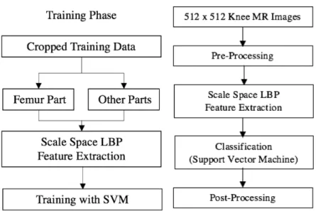
The proposed approach consists of two phases: training phase and segmentation phase. In the training phase, the SSLBP feature is extracted for obtaining special texture characteristics of bone parts and train them with a SVM classifier. In the next step, segmentation phase, knee MRI scans are pre-processed firstly to remove artifacts from the background of images and improve their qualities. After that, each pixel's feature is extracted based on the previously defined feature extraction method, SSLBP. The pre-processed image is classified into the bone part and other parts by the SVM. The resulting image from the classification step is post-processed by fuzzy c-means methodology. Fig. 1 illustrates our proposed model.
The rest of paper is organized as follows. Section 2 explains briefly about the Support Vector Machine and Feature extraction which are related with our proposed methodology. Section 3 reviews several knee segmentation techniques. Our proposed methodology is described in Section 4, and the experimental results are demonstrated in Section 5. Section 6 presents our main conclusion.
2. LITERATURE REVIEW
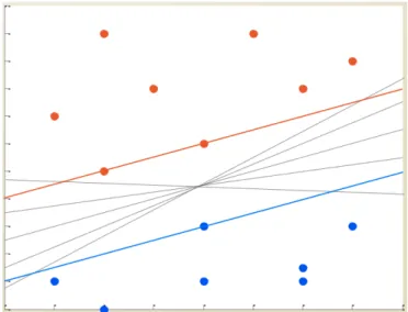
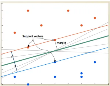
Support Vector Machine (SVM) is an effective method for general-purpose pattern recognition proposed recently, which developed by V.Vapnik and his team(AT&T Bell Labs). Intuitively, a SVM finds a hyperplane that is placed between two classes and as far as possible from both sides in a set of given points belonging to two classes [27][28][29][30]. Fig. 2 shows an example of two classes with vectors. There are several gray lines that can be the hyperplane between two classes. To be an optimal hyperplane, the one with the maximum margin of separation between the two classes, where the margin is perpendicular distance from the closest point to the decision boundary between support vectors and itself. These closest data points are called Support Vectors (SVs) [31]. Based on these, Fig. 3 shows that the found decision boundary (green line) between two classes with vectors (red and blue dots). SVM finds vectors that support decision boundary which called support vectors with maximum margin.
Figure 3: An example of basic concept of Support Vector Machine with found decision boundary
Feature extraction is initially performed in binary classification problem [31]. In the texture analysis process, feature extraction is the main and specific step, as well as, selection of a feature extraction method is one of the most important factors in achieving high recognition performance [32][33].
3. RELATED WORK
Various segmentation methods in respect to the knee bone are adopted in research and clinical practices such as thresholding, region growing, deformable models, clustering methods, and Atlas guided approaches [10].
Lee et al. describe methods of bone extraction using thresholding [11, 12]. Image thresholds are strength-based methods and provide a simple, less computationally expensive segmentation of the knee image that can be applied either globally or locally. However, non-uniform acquisition of MRI scans unfortunately cannot be used for quantitative purposes [10]. The region-based segmentation is one of the most popular approaches to extract the bones from knee MRI scans because the knee bones utilize more space than other structures [14]. Dalvi et al. introduced the models using region growing algorithms combined with other methodologies such as fuzzy c-means and thresholding [11, 13]. However, leakage is often generated by region growing methods in tissues external to the segmented Region of Interest (ROI) during clinical assessments. One of the most popular methods is the Fuzzy c-means clustering algorithm (FCM). It works by clustering feature vectors by minimizing the objective function composed of the membership functions and the similarity between the center of the cluster and the measured data [13, 15]. A known drawback of FCM, however, is high noise sensitivity because it considers only difference in intensity levels. Since significant uncertainties and unknown noise are always included in medical images, degradation with segmentation generally occurs [15]. Many researchers have studied FCM, and related extensions have been developed to solve this problem. For instance, IFCM is an Improved FCM model proposed by Bezdek et al. [15, 16] which considers the entire local neighborhood. To optimize
parameters, however, IFCM requires additional processes. An algorithm that modifies the objective function of the FCM has been introduced called FCM_S. Labeling which one is affected by neighboring pixels is allowed to compensate for the homogeneity of the intensity under this algorithm [17, 18]. Gaussian noise or salt and pepper noise in images have been alleviated by the above FCM algorithm. It does not, however, solve the problem of bones with knee MRI texture problems.
Ambellan et al. segment knee bone and cartilage by combining statistical shape knowledge and Convolutional Neural Networks (CNN) [19]. Neural network is one of techniques widely used in image processing; nevertheless, their learning process is affected by the size of the dataset [20]. Thus, the pre-trained networks are usually used to fine-tune with the limited dataset.
4. PROPOSED MODEL
Since features can contain essential information from images, extracting features from an image is important, and therefore detection of features is an important step in image segmentation [21]. In our proposed framework, we concentrate on the knee bone segmentation using SSLBP feature extraction from MRI scans. Our proposed method's segmentation pipeline is shown in Fig. 4.
The main purpose of training phase is to define special features for detecting the bone which has a texture problem with cropped training dataset and trains it. Based on this trained data, in the segmentation phase, we pre-process the knee MRI scans before extracting features for each pixel. After that, we use a SVM to classify the image into the bone part and other parts. The resulting image of classification is post-processed.
4.1 TRAINING PHASE 4.1.1 Cropped Training Data
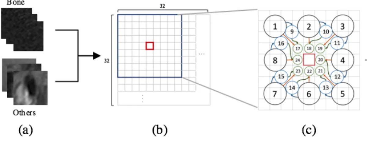
Segmentation of textured organs is a difficult process since texture features often cannot provide sufficient discrimination to allow accurate segmentation [9]. In order to better provide discrimination between the knee bone part and other parts, the input images are cropped into a window size of 32x32 that has been arbitrarily chosen. A total of 11,459 images (5,695 images for the bone part and 5,764 images for other parts) are collected and used in the training phase. Fig. 5 shows the example cropped images of bone parts (Fig. 5 (a)-(e)) and other parts (Fig. 5 (f)-(j)).
Figure 5: Example cropped images of (a)(b)(c)(d)(e) bone parts (f)(g)h)(i)(j) other parts.
4.1.2 Feature Extraction
As we can see on Fig. 5 examples, there are a large number of blobs in the images of bone parts. In addition to the large number of blobs, the overall intensity is also lower than the images of other parts. Several images of other parts also include various blobs in the images, but there is a significant difference from the bone part images in terms of intensity
and it is distinguished from the bone part images by the number of blobs and the intensity difference between blocks and surrounding pixels.
In order to extract features that characterize the texture of the knee bone at each pixel based on above difference, a window size of 9x9 is used as shown in Fig. 6(c). This is a size that shows the imbalance of the intensity that appears specifically in the bone part, and the feature is extracted based on the window size. The 9x9 window moves through the 32x32 image (Fig. 6 (b)) and extracts the features for each pixel.
Figure 6: Set up the window size for feature extraction, (a) cropped input images (bone and other parts), (b) demonstrate that the 9x9 window inside of 32x32 window, (c)
and 9x9 window which is utilized for extracting features
As mentioned above, the specific feature of the bones is the imbalance of intensity. Utilizing the characteristic of intensity imbalance of the knee bone, we attempt to extract the feature that differentiates it from other parts. To extract the feature corresponding to each pixel, we first decompose it in various scale sizes to extract pixel information around
the target pixel, 3x3 scale windows (𝐴𝑟𝑒𝑎1 − 𝐴𝑟𝑒𝑎8), 2x2 scale windows (𝐴𝑟𝑒𝑎9 −
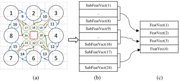
Among those extracted various scale windows, we first declared the intensity difference with the nearest neighbors, not at the same level as itself. The arrows in Fig. 7(c) indicate pairs that are compared and the differences between pairs are saved into 𝑆𝑢𝑏𝐹𝑒𝑎𝑡𝑉𝑒𝑐𝑡. The arrows in Fig. 7(a) between objects imply the relationship of the comparison objects.
Figure 7: Feature Vector description (a) Feature Extraction Window, (b) Sub-feature vector, (c) and extracted Feature Vector
After that, a final feature vector, 𝑓𝑒𝑎𝑡𝑉𝑒𝑐𝑡, is extracted using the comparison of
average of the intensity differences for each level to reduce the size of the feature vector as shown in Fig. 7(c). The comparison utilized the following rules:
a𝑣𝑔𝐼𝑛𝑡𝑠𝑡(𝑛) < 𝑎𝑣𝑔𝐼𝑛𝑡𝑠𝑡(𝑚) − 𝛿, f𝑒𝑎𝑡𝑉𝑒𝑐𝑡(𝑘) = 0 𝑎𝑣𝑔𝐼𝑛𝑡𝑠𝑡(𝑚) − 𝛿 ≤ 𝑎𝑣𝑔𝐼𝑛𝑡𝑠𝑡(𝑛)
≤ 𝑎𝑣𝑔𝐼𝑛𝑡𝑠𝑡(𝑚) + 𝛿,
f𝑒𝑎𝑡𝑉𝑒𝑐𝑡(𝑘) = 1 (1)
𝑎𝑣𝑔𝐼𝑛𝑡𝑠𝑡(𝑚) + 𝛿 < 𝑎𝑣𝑔𝐼𝑛𝑡𝑠𝑡(𝑛), f𝑒𝑎𝑡𝑉𝑒𝑐𝑡(𝑘) = 2
𝑛, 𝑚 indicates the area number; 𝑎𝑣𝑔𝐼𝑛𝑡𝑠𝑡(𝑛) is the average intensity of each scale
levels; 𝛿 is a constant value to show the flatness of the image; 𝑘 represents the position of
the 𝑓𝑒𝑎𝑡𝑉𝑒𝑐𝑡 where the comparison value is stored, and 𝑓𝑒𝑎𝑡𝑉𝑒𝑐𝑡 is the final feature vector of SSLBP feature extraction which contains the current pixel’s intensity and the values of comparison of the average intensity of each scale levels.
4.1.3 Training with SVM
Support Vector Machine (SVM) is a modern classification algorithm that is an attractive choice in computerized image processing. The classification of MRI scans to its related class is a primary utilization of SVM. Machines are trained via the tasks performed by SVM to find the optimal hyperplane which assigns the maximum distance to the closest point of data of any class from the training datasets [22, 23]. Extracted SSLBP feature is used as the input data of the SVM to train for classification. We have trained a SVM classifier provided in MATLAB with linear kernel option and the training accuracy was 94.78%.
4.2 SEGMENTATION PHASE 4.2.1 Pre-Processing
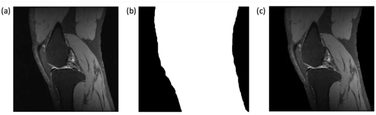
To improve visual appearance and image quality for better efficiency and accuracy of the proposed model, pre-processing step should be utilized before classification step. In this pre-processing step, we focus on removing noise from the background and use the same pre-processing method used in [24]. For removing the noise, firstly we extract the ROI Mask from the image with a process, and it is as follows. Convert input original images to binary images; objects smaller than a specific size is removed from the binary images by using a morphological operation, and then morphologically close the image with small objects removed. Using the extracted ROI binary mask, only pixels which correspond to white pixels are kept from the original images. Thus, only the area that represents the knee is kept and the background is cleaned by setting to a zero. Fig. 8 shows the result image of pre-processing step (Fig. 8(c)) with original image (Fig. 8(a)) and its ROI mask image (Fig. 8(b)).
Figure 8: The result image of pre-processing step (a) Original image (b) ROI mask image and (c) pre-processed image
4.2.2 Feature Extraction & Classification
After improving image qualities from the pre-processing step, SSLBP feature extraction is used to extract features for each pixel in the entire image. A 9x9 window passes through the 512x512 original knee MRI image, extracts feature of the center pixel of the window, and this feature will be used in the SVM classifier as input vectors. In the classification phase, the SVM classifier provided in MATLAB was also used with default values for optional parameters. In the classification phase, we used different images than the trained data.
Figure 9: The result of SVM classification with SSLBP feature extraction (a) Pre-processed Image, (b) The Result of classification, (c) and extracted bone from the
classification phase
The images in Fig. 9 show the result of SVM classification with SSLBP feature extraction. Fig. 9(a) is the pre-processed image which is used as an input for SVM classification. Fig. 9(c) is the result of extraction displaying only the parts that have been classified as bones, and the small objects that belong to other parts of the bone were deleted from Fig. 9(b) which is the original SVM classification result.
4.2.3 Post-Processing
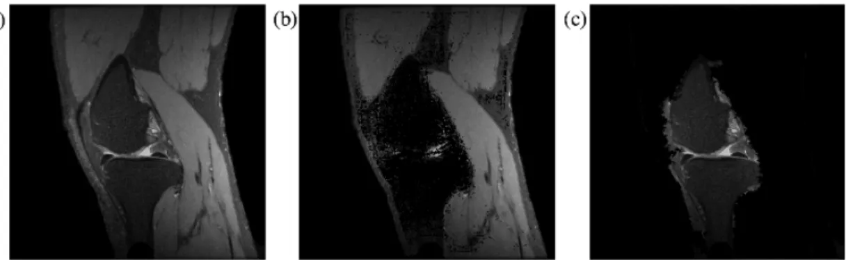
The classified result as the bone part includes bones, cartilage, and several pixels which do not belong to bone around the bones. For the first step of post-processing, we convert the result from the previous step to binary image to remove unwanted small objects. However, the result image after removing the unwanted small objects still have not only the bone part but other parts also, as shown in Fig. 10(a). Since other parts have distinctive higher intensity value than the bone parts without similar texture problem, we performed fuzzy c-means clustering to segment the bone part and others. Fig. 10 shows the entire clustering process.
Figure 10: The result images (a) The image after removed small unwanted objects from the classified result, the result of binary image (b) for bone parts, (c) for other parts
5. EXPERIMENTAL RESULTS AND ANALYSIS
The proposed model was evaluated by using the confusion matrix for measuring Accuracy (ACC) and Matthews Correlation Coefficient (MCC).
MCC is used as a quality measure of binary classification in machine learning. It returns the value between -1 and 1, where the coefficient of +1 represents the perfect prediction, 0 is worse than the random prediction, and -1 represents the total discrepancy between prediction and observation. For normalization purposes, it is multiplied by 100.
𝑀𝐶𝐶 = 𝑇𝑃 ∗ 𝑇𝑁 – 𝐹𝑃 ∗ 𝐹𝑁
O(𝑇𝑃 + 𝐹𝑃)(𝐹𝑃 + 𝐹𝑁)(𝑇𝑁 + 𝐹𝑃)(𝑇𝑁 + 𝐹𝑁)∗ 100
(2)
ACC indicates the systematic error that is a measure of the statistical bias.
𝐴𝐶𝐶 = (𝑇𝑃 + 𝑇𝑁)
𝑇𝑃 + 𝐹𝑃 + 𝑇𝑁 + 𝐹𝑁 ∗ 100
For these evaluations, the result images with ground truth were compared pixel by pixel, and counted the number of the pixels that belong to these categories:
TABLE 1: Definition of each category for comparison
Labels Meaning
TP (True Positive) Bones correctly identified as bones
TN (True Negative) Other parts correctly identified as other parts
FP (False Positive) Other parts correctly identified as bones
FN (False Negative): Bones incorrectly identified as others
The proposed method was compared with fuzzy c-means clustering algorithm which is intensity-based methodology, and deep feature extraction methodology that uses a pre-trained Deep Neural Network (DNN) with ImageNet [26]. The DNN was repre-trained with our training data and extracted feature to classify. The classified image from deep feature extraction method was post-processed, as in the proposed method.
We used an online MRI data set obtained at [25] for the proposed method to train and classify. The MRI dataset also had been used for experiments result comparison with three methods. The ground truth was manually generated by domain experts for evaluation.
For a reasonable result comparison, we did not include the number of background pixels in evaluation calculation. Fig. 14 shows the result knee bone extraction using the fuzzy c-means algorithm (Fig. 14 (d)(e)(f)), deep feature extraction methodology (Fig. 14 (g)(h)(i)) and the proposed approach (Fig. 14 (j)(k)(l)). The input image for an experimental result made use of different images from trained data set. Table 2 shows the average percentages of each category of results and Table 3 represents the result of both confusion matrix analysis of existing methods, fuzzy c-means, and deep feature, and proposed method.
TABLE 2: Average percentage of each category TP (%) TN (%) FP (%) FN (%) Ground Truth 19.1 80.9 - - Fuzzy c-means 15.4 67.4 13.5 3.6 Deep feature 8.5 79.12 1.8 10.6 Proposed model 17.3 78.8 2.1 1.8
TABLE 3: Results of ACC and MCC evaluation
ACC (%) MCC (%)
Fuzzy c-means 82.93 60.04
Deep feature 87.67 57.14
Proposed model 96.10 88.26
The results of our proposed approach have higher ACC and MCC values compared to intensity-based methods, especially on MCC result as shown in Table 3. As represented in
Equation 2, the 𝐹𝑃 ∗ 𝐹𝑁 value on the second term of numerator has a great influence on
the MCC result, and our proposed method has less 𝐹𝑃 and 𝐹𝑁values than the other two.
These experimental results show that the SSLBP feature extraction applied to SVM is superior to existing intensity-based image processing tools such as fuzzy c- means algorithm. Also, the SSLBP features which extracted from our intuition in the proposed method outperforms the extracted features from DNN with ImageNet [26].
As well as, we compared the results with different size of training data and different size of cropped image. Firstly, the result comparison of two different size of training data is shown, total 11,459 images which contains 5,695 images for bone part and 5,764 images for other parts and total 21,506 images which contains 10,578 images for bone part and 10,928 image for other parts. This experiment result comparison also did not include the background pixels in evaluation calculation. Fig. 13 shows the result of knee bone extraction trained with about a thousand images (Fig. 13 (a)(b)) and with about two thousand images (Fig. 13 (c)(d)). Table 4 shows the percentages of each category of results and Table 5 represents the result of both confusion matrix analyses.
TABLE 4: Average percentage of each category for two different size of trained data
Approximate Number of images
TP (%) TN (%) FP (%) FN (%)
A thousand 17.3 78.8 2.1 1.8
TABLE 5: Results of Training Accuracy, ACC and MCC evaluation for two different size of trained data
Approximate Number of images Training Accuracy ACC (%) MCC (%) A thousand 94.78 96.10 88.26 Two thousands 93.67 94.40 81.38
Figure 12: Comparison of Training Accuracy, ACC and MCC evaluation for two different size of trained data
Next, we extracted SSLBP features from 16x16 size of cropped images and trained SVM. The result using 16x16 cropped image size has less training accuracy compared with 32x32 size of cropped image. Table 6 shows the training accuracy comparison result of
16x16 cropped image and 32x32 cropped image. As the result represents, the smaller size of cropped image has lower performance for training SVM.
TABLE 6: Results of Training Accuracy for two different size of cropped image
Cropped Image Size Training Accuracy
16x16 size images 74.48
32x32 size images 94.78
In addition, the time to detect feature in 64x64 cropped image has been compared with the time in 32x32 cropped image. Since feature is detected at each pixel in the image, the size of feature for an image is 2,917 in a 32x32 image, and 13,925 in a 64x64 image. We estimate the running times to detect feature in each size of image with 5 attempts and Table 7 shows the result of estimated running times.
TABLE 7: Results of Training Accuracy for two different size of cropped image
32x32 image(seconds) 64x64 image(seconds) 1 0.03746 0.20244 2 0.03574 0.17353 3 0.03643 0.17316 4 0.03579 0.17158 5 0.03572 0.16911 Average 0.03623 0.17796
As Table 7 shows using 32x32 images has about 6 times faster to detect feature than using 64x64 images. Based on these experimental results, the 32x32 image works faster on feature detection and with higher training accuracy.
We have used a MRI data set obtained from [25] for the proposed method to train and classify. The MRI dataset also had been used for experiments result comparison with three methods. The ground truth was manually generated by domain experts for evaluation.
Figure 13: The result comparison images with difference size of training dataset (a) The result of classification with about a thousand images, (b) the final knee bone
extraction result with about a thousand images, (c) The result of classification with about two thousand images, (d) the final knee bone extraction result with about two
Figure 14: The result images for comparison (a),(b),(c) the ground truth images, (d),(e),(f) the result of fuzzy c-means methodology, (g),(h),(i) the result of deep
6. CONCLUSIONS
Knee is an area primarily responsible for supporting the total weight of human body, and precise segmentation of bones in MRI plays a crucial role in clinical studies [3, 4]. However, some MR images make it difficult to study clustering due to knee bones texture problem [13]. In this paper, we employed the SSLBP feature extraction, a variant of local binary pattern, to train and classify the pre-processed MRI scans using SVM. The proposed approach uses the SSLBP feature extraction to train and classify the pre-processed MRIs with SVM, and the post processing step is done with the classified image. The experimental result showed that our approach had higher ACC and MCC values, compared to fuzzy c-means and deep feature extraction methods. The precise knee bone detection through the proposed model would be an important assist in the development of a fully autonomous surgical system[1, 2, 3].
BIBLIOGRAPHY
[1] E. J. Park, M. S. Cho, S. J. Baek, H. Hur, B. S. Min, S. H. Baik, K. Y. Lee, and
N. K. Kim. 2016. Long-term oncologic outcomes of robotic low anterior resection for rectal cancer: a comparative study with laparoscopic surgery. Post-publication peer review of the biomedical literature.
[2] C.B. Chng, Y. Ho, and C.K. Chui. 2015. Automation of retinal surgery: A shared
control robotic system for laser ablation. 2015 IEEE International Conference on Information and Automation.
[3] J. Fripp, S. Crozier, S. K. Warfield, and S. Ourselin. 2007. Automatic
segmentation of the bone and extraction of the bone–cartilage interface from magnetic resonance images of the knee. Physics in Medicine and Biology, vol. 52, no. 6, pp. 1617–1631.
[4] J. Schmid and N. Magnenat-Thalmann. 2008. MRI Bone Segmentation Using
Deformable Models and Shape Priors. Medical Image Computing and Computer-Assisted Intervention – MICCAI 2008 Lecture Notes in Computer Science, pp. 119–126.
[5] A. R. Lanfranco, A. E. Castellanos, J. P. Desai, and W. C. Meyers. 2004. Robotic
Surgery A Current Perspective, Lippincott Williams & Wilkins.
[6] A. J. Teichtahi, A. E. Wluka, M. L. Dabies, and F. M. Cicuttini. 2008. Imaging
of knee osteoarthritis. Best Pratice & Researcj Clinical Rheumatology, vol. 22, no. 6, pp.10651-1074.
[7] B. Pirzamanbin, A fully automated segmentation of knee bones and cartilage using shape context and active shape models. Lund: Lund University, 2012.
[8] T. G. Williams, A. P. Holmes, J. C. Waterton, R. A. Maciewicz, C. E.
Hutchinson, R. J. Moots, A. F. P. Nash, and C. J. Taylor. 2010. Anatomically Corresponded Regional Analysis of Cartilage in Asymptomatic and Osteoarthritic Knees by Statistical Shape Modelling of the Bone. IEEE Transactions on Medical Imaging, vol. 29, no. 8, pp. 1541–1559.
[9] P. Bourgeat, J. Fripp, P. Stanwell, S. Ramadan, and S. Ourselin. 2007. MR image
segmentation of the knee bone using phase information. Medical Image Analysis, vol. 11, no. 4, pp. 325–335.
[10] A. Aprovitola and L. Gallo. 2016. Knee bone segmentation from MRI: A classification and literature review. Biocybernetics and Biomedical Engineering, vol. 36, no. 2, pp. 437–449.
[11] R. Dalvi, R. Abugharbieh, D. Wilson, and D. R. Wilson. 2007. Multi-Contrast MR for Enhanced Bone Imaging and Segmentation. 2007 29th Annual International Conference of the IEEE Engineering in Medicine and Biology Society.
[12] J.S. Lee and Y.N. Chung. 2005. Integrating Edge Detection And Thresholding Approaches To Segmenting Femora And Patellae From Magnetic Resonance Images. Biomedical Engineering: Applications, Basis and Communications, vol. 17, no. 01, pp. 1–11.
[13] J. Y. Mun, J. Y. Lee, D. Y. Kim, and S. Shin. 2017. Extract texture-problematic femur from Knee MRI using Fuzzy C-means and Region Growing approach. International Conference on Internet.
[14] Y. Sun, E. C. Teo, and Q. H. Zhang. 2007. Discussions of Knee joint segmentation. Biomedical and Pharmaceutical Engineering, 2006. ICBPE 2006. International Conference on. IEEE 2006.
[15] J. C. Bezdek. Pattern recognition with fuzzy objective function algorithms. Springer Science & Business Media, 2013
[16] S. Shen, W. Sandham, M. Granat, and A. Sterr. 2005. MRI Fuzzy Segmentation of Brain Tissue Using Neighborhood Attraction With Neural-Network Optimization. IEEE Transactions on Information Technology in Biomedicine, vol. 9, no. 3, pp. 459–467.
[17] S. Chen and D. Zhang. 2004. Robust Image Segmentation Using FCM With Spatial Constraints Based on New Kernel-Induced Distance Measure. IEEE Transactions on Systems, Man and Cybernetics, Part B (Cybernetics), vol. 34, no. 4, pp. 1907–1916.
[18] L. Szilagyi, Z. Benyo, S. Szilagyi, and H. Adam. MR brain image segmentation using an enhanced fuzzy C-means algorithm. Proceedings of the 25th Annual International Conference of the IEEE Engineering in Medicine and Biology Society (IEEE Cat. No.03CH37439).
[19] F. Ambellan, A. Tack, M. Ehlke, and S. Zachow. April, 2018. Automated Segmentation of Knee Bone and Cartilage combining Statistical Shape Knowledge and Convolutional Neural Networks: Data from the Osteoarthritis Initiative. Venues.
Available: https://openreview.net/forum?id=SJ_-Nx3jz.
[21] S. Udomhunsakul and P. Wongsita. 2004. Feature extraction in medical MRI images. IEEE Conference on Cybernetics and Intelligent Systems.
[22] K. D. Kharat, V. J. Pawar, and S. R. Pardeshi. 2016. Feature extraction and selection from MRI images for the brain tumor classification. International Conference on Communication and Electronics Systems (ICCES).
[23] E. B. George and M. Karnan. 2012. MRI Brain Image Enhancement Using Filtering Techniques. International Journal of Computer Science & Engineering Technology (IJCSET). Vol. 3 No. 9, 399-403.
[24] J. Y. Lee, J. Y. Mun, M. Taheri, S. H. Son, and S. Shin. 2017. Vessel Segmentation Model using Automated Threshold Algorithm from Lower Leg MRI. Proceedings of the International Conference on Research in Adaptive and Convergent Systems - RACS 17.
[25] “MRI Data,” MRI Data. [Online]. Available: http://mridata.org/fullysampled [26] A. Krizhevsky, I. Sutskever, G. E. Hinton. 2012. ImageNet Classification with
Deep Convolutional Neural Networks. Communications of the ACM, vol. 60, no. 6, 84–90.
[27] E. Osuna, R. Freund, and F. Girosit. 1997. Training support vector machines: an application to face detection. Proceedings of IEEE Computer Society Conference on Computer Vision and Pattern Recognition.
[28] M. Pontil and A.Verri. 1998. Support Vector Machines for 3D Object Recognition. IEEE Transactions on Pattern Analysis and Machine Intelligence, vol. 20.
[29] C. Cortes and V.N. Vapnik. 1995. Support Vector Network. Machine Learning, vol. 20, pp. 1-25.
[30] V. N. Vapnik, The nature of statistical learning theory. New York: Springer, 2010.
[31] H. Byun and S.W. Lee. 2002. Applications of Support Vector Machines for Pattern Recognition: A Survey. Springer.
[32] Ø. D. Trier, A. K. Jain, and T. Taxt, Feature extraction methods for character recognition-A survey. Pattern Recognition, vol. 29, no. 4, pp. 641–662, 1996. [33] A. Larroza, V. Bodí, and D. Moratal. 2016. Texture Analysis in Magnetic
Resonance Imaging: Review and Considerations for Future
Applications. Assessment of Cellular and Organ Function and Dysfunction using Direct and Derived MRI Methodologies.