A Probabilistic Methodology for Quantifying, Diagnosing and Reducing
Model Structural and Predictive Errors in Short Term Water Demand
Forecasting
Christopher J. Huttona,b,* and Zoran Kapelana
a Water and Environmental Management Research Centre, Department of Civil Engineering, Queen's School of
Engineering, University of Bristol, Queen's Building, University Walk, Bristol BS8 1TR, UK. Email: [email protected]
bCentre for Water Systems, College of Engineering, Mathematics and Physical Sciences, University of Exeter, UK. Email:
*corresponding author
Abstract
Accurate forecasts of water demand are required for real-time control of water supply systems under normal and abnormal conditions. A methodology is presented for quantifying, diagnosing and reducing model structural and predictive errors for the development of short term water demand forecasting models. The methodology (re-)emphasises the importance of posterior predictive checks of modelling assumptions in model development, and to account for inherent demand uncertainty, quantifies model performance probabilistically through evaluation of the sharpness and reliability of model predictive distributions. The methodology, when applied to forecast demand for three District Meter Areas in the UK, revealed the inappropriateness of simplistic Gaussian residual assumptions in demand forecasting. An iteratively revised, parsimonious model using a formal Bayesian likelihood function that accounts for kurtosis and heteroscedasticity in the residuals led to sharper yet reliable predictive distributions that better quantified the time varying nature of demand uncertainty across the day in water supply systems.
Keywords: Water Demand; Forecast; Model Calibration; Uncertainty; Bayesian; Real Time.
1.
Introduction
Understanding natural variability in urban water demand, the fundamental aleatory uncertainty affecting water supply systems (Hutton et al., 2012), helps water utilities to satisfy consumer demand, whilst at the same time allowing them to try and minimise the costs associated with supplying sufficient water. Over decadal scales estimates of future water demand support strategic planning, allowing utilities to understand potential water shortages relating to climatic changes, and make capital investments in the water distribution
and treatment infrastructure to meet future demand (Qi and Chang, 2011; Almutaz et al., 2013). At shorter time-scales predicted water demand up to several days ahead forms a key input to near real-time control systems, and can contribute towards the reduction of energy consumption and cost associated with supplying water in distribution networks (Martinez et al., 2007; Bakker et al., 2013). Furthermore, short term predictions of urban water consumption are important for burst detection, helping utilities to distinguish between actual demand and non-revenue water (Mounce et al., 2010).
Existing short-term Water Demand Forecasting (WDF) research (e.g. < 48 hours), has mainly focussed on two aspects of the forecasting problem: identification of the best inputs to predict future demand - both endogenous and exogenous variables - and on identification the best model structures to map these input variables to predict future demand (Adamowski, 2008; Herrera et al., 2010). Relatively few approaches, however, have attempted to quantify the uncertainty in demand forecasts over shorter timescales (Cutore et al., 2008), despite the fact that water demand is highly uncertain due to: (a) a range of difficult to constrain socio-demographic and economic factors known to affect water consumption (Arbués et al., 2003), which themselves vary both spatially and temporally; (b) the fact that residential demand is often not fully metered (e.g. <40% properties in the UK). Even when properties are metered, often they are not read frequently enough to quantify short term demand fluctuations. Demand uncertainty needs to be quantified adequately as it will propagate adversely to affect the accuracy of subsequently derive models, forecasts and control decisions (Hutton et al., 2013; Hutton et al., 2014). The relative performance of demand forecasting models has typically been evaluated and compared with reference to global metrics of model performance such as Root Mean Square Error (RMSE; e.g. Herrera et al., 2010) that summarise model performance in an average sense over the whole dataset. Such metrics reveal little information about how a model performs poorly, where the key errors in model performance lie, and therefore provide little guidance upon how models may be improved. Furthermore, the statistical assumptions upon which demand forecasting model calibration that employs metrics such as RMSE is typically based (e.g. independent, and identically distributed (iid) Gaussian errors) are seldom reported, and therefore evaluated, in the demand forecasting literature. This is despite the fact that it is on the validity of these statistical foundations that the legitimacy of any model comparison is based.
Building upon the work of Hutton et al. (2014), who presented a framework for considering the cascade of uncertainty from model calibration, through forecasting, to real time control in Water Supply Systems, this paper presents a probabilistic methodology for the development and calibration of short water demand forecasting models. The methodology is designed to develop more reliable short term WDF models, and provide quantitative information on model predictive uncertainty to the decision maker. A Bayesian approach is applied for model parameter calibration, and subsequent posterior predictive uncertainty quantified
probabilistically. The framework emphasises the iterative application of residual error analysis during calibration, and evaluation of the reliability and sharpness of the predictive distributions in order to diagnose errors within the model structure and errors in the residual error assumptions made during calibration. Section 2 reviews short term water demand forecasting; Section 3 presents the overall methodology, followed by a case study implementing the methodology to forecast demand for 3 District Meter Areas in the UK; Sections 4 and 5 then discuss and conclude the paper, respectively.
2.
Short Term Water Demand Forecasting and Model development
Short term WDF modelling research has generally focussed on identifying the best model inputs, and on identifying the best models to combine these inputs and map them to predict future water demand. Approaches have applied either endogenous variables - e.g. past values of water demand (Alvisi et al., 2007; Cutore et al., 2008; Romano and Kapelan, 2014) – and/or exogenous variables such as temperature and precipitation (Zhou et al., 2002; Herrera et al., 2010; Adamowski, 2008). Unless past weather variables are used, temperature and precipitation variables may need to be forecasted as inputs to the demand forecasting model, which will contain additional uncertainty. Furthermore, as pointed out by Bakker et al (2013b) it may be difficult to include weather variables reliably in a practical setting due to reliance on external systems.
A number of different data driven modelling approaches have been applied for short term WDF including multi-linear regression (MLR), Autoregressive (Integrated) Moving Average models (AR(I)MA (Adamowski, 2008; Zhou et al., 2002), and non-linear methods including multiple non-linear regression (MNLR; Adamowski et al., 2012), Artificial Neural Networks (ANNs; Romano and Kapelan, 2014) and variants thereof including dynamic ANNs (Ghiassi et al., 2008), Wavelet transform (WA-) ANNs (Adamowski et al., 2012), and Support Vector Machines (SVM; Herrera et al., 2010). A final class of models that may be considered more heuristic in approach have structures built upon observations made from exploratory data analysis. Such models share similarities with ARMA approaches, and generally include a component representing the average behaviour of the system, such as an average of past water demands (Herrera et al., 2010), and a persistence component representing local deviations in time, which may be represented through regression on recent prediction errors (Alvisi et al., 2007). Bakker et al. (2013b) applied a heuristic approach in which normalised water demands are used as input variables and combined with multipliers for the specific day of the week, and time of day to derive the forecast.
A number of papers have conducted comparative analysis between different data driven models; Adamowski et al (2008) found that ANNs outperform linear regression and ARIMA models for peak daily water demand forecasting. SVM models have also be found to outperform 5 other model structures for one hour ahead demand forecasts (Herrera et al., 2010), whilst WA-ANNs have been found to outperform MLR, MNLR, AIRMA
and ANN models for daily water demand forecasting (Adamowksi et al., 2012). However, in this latter approach wavelet transformed data could also be applied as input to other model types. Whilst it is difficult to compare different WDF methodologies in different contexts, Mean Absolute Percentage Errors (MAPE) reported in the literature generally vary between 3 to 10% for lead times up to 24 hours (Bakker et al., 2013; Romano and Kapelan, 2014; Alvisi et al., 2007), where the lowest errors reported by Bakker et al. (2013b) were found in the larger supply zones where deviant behaviour from the norm is more likely to be masked by average behaviour.
The relative performance of different WDF models has been judged mainly with reference to global metrics of model performance like MAPE, including Root Mean Square Error (RMSE), and Mean Absolute Error (MAE; Ghiassi et al., 2008; Herrera et al., 2010). Such metrics, however, provide limited scope for comparative analysis as they collapse all residual error information into a single value, and can therefore only tell us how good models are in an average sense. Gupta et al. (2008) argue that such metrics are therefore weak in a diagnostic sense, as they reveal little information about how and where within a simulation a model performs poorly. Such metrics therefore provide limited information to determine between competing models, and guide subsequent model improvement.
To overcome the problems of model evaluation solely with global metrics, further investigation of the residual errors is required. Such exploration is important for two reasons. First, it is important to test the assumptions of Gaussianity, heteroscedasticity and independence of residual errors that are (implicitly) assumed during the model fitting exercise (Engeland et al., 2005). This is particularly important as it is on these assumptions that the validity of the model fit, and in turn the validity of any subsequent model comparison, is based. Second, context specific residual error analysis helps to identify how and where a model performs poorly. Residual analysis, however, is not routinely applied (or at least not fully reported) in the literature during WDF model development.
A further need to analyse in more details the residual errors is that urban water demand is highly uncertain due to limited spatial and temporal metering coverage, and also because of a range of factors that influence water consumption (and leakage), which themselves vary spatially and temporally (Arbués et al., 2003). Water demand uncertainty is also the key aleatory uncertainty that propagates into, and influences that accuracy of Water Distribution System model predictions (Hutton et al., 2014). However, despite this uncertainty, and despite the wider application of uncertainty quantification methods in Urban Water Systems’ modelling (Kapelan et al., 2007; Alvisi and Francini, 2010; Hutton et al., 2013; Hutton et al., 2014; Breinholt et al., 2012; Deletic et al., 2012) and hydraulic/hydrological modelling more generally (Liu and Gupta, 2007; Beven, 2008), few approaches have moved beyond deterministic WDF modelling. In a forecast setting, where models are to be applied to inform decision making, quantification of the reliability of a model prediction provides important additional information. One exception is Cutore et al. (2008) who applied the SCEM-UA algorithm within a
Bayesian framework to calibrate an ANN for daily water demand forecasting. The approach was used to quantify probabilistically parameter and posterior predictive uncertainty. However, no posterior analysis was applied to evaluate the assumptions made during model calibration, nor was any evaluation of the quality of the model predictive bounds made. A key and often neglected aspect of formal Bayesian calibration is to assess whether the residuals can be represented by a statistical likelihood function. Such simplistic assumptions can break down in the context of WDS modelling (e.g. Hutton et al., 2013), as residual distributions are often coloured (Beven et al., 2011): that is they contain bias, with structured, auto-correlated errors resulting from epistemic uncertainty, which can lead to poorly calibrated models and unfair estimates of model predictive uncertainty. In a forecasting setting where models are to be applied in decision making context – e.g. for burst detection or pump scheduling – the frequentist properties of the predictive distribution can be checked during both calibration and validation to understand the robustness and sharpness of the model prediction bounds (Breinholt et al., 2012).
3.
Water Demand Forecast Model Development Methodology
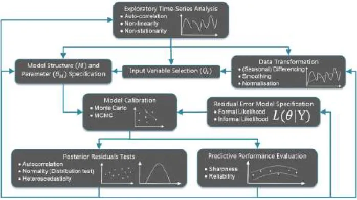
The presented probabilistic methodology for the development and calibration of short term WDF models is outlined in Figure 1. The aim of the methodology is to obtain, through iterative feedback between model development, calibration and performance evaluation, parsimonious yet reliable predictive models of future water demand over short forecasting horizons (e.g. < 24 hours). In this sense, the methodology (re-) emphasises that model fitting is a scientific exercise of hypothesis testing (Box, 1976), where the hypothesised model is confronted with data. Central to the methodology is the application of appropriate posterior predictive checks using metrics with diagnostic power (Gupta et al., 2008) to identify discrepancies between data and model. Such checks may lead to model rejection (falsification), in the sense that we identify parts of the model that don’t fit (e.g. Residual Autocorrelation; Bennett et al., 2013). Such identification then provides guidance on how the model may be improved. As all models are wrong, one cannot obtain a correct model. Rather, the aim is to obtain iteratively, through exploratory analysis, model testing, and diagnosing model errors, a better, useful model (Gelman and Shalizi, 2013; Box, 1976). A key aspect of the methodology is the recognition of the inherent aleatory and epistemic uncertainties in water demand forecasting. Therefore, an ensemble forecasting approach is adopted, as often applied in flood forecasting (Cloke and Pappenberger, 2009), where the quality of the model forecasts are quantified not in terms of deterministic metrics of model performance, such as RMSE, but rather in terms of the reliability and sharpness of the predictive distributions (Breinholt et al., 2012). Further details of the overall methodology are considered here, with more specific methodological decisions made at each stage of model development (Figure 1) elaborated in the context of a specific case study of water demand forecasting for three District Meter Areas (DMAs) in the UK.
Figure 1. Flow diagram of the iterative steps involved in the model development methodology.
3.1 Exploratory Time-Series Analysis
Exploratory analysis of different time-series and their suitability as inputs to predict the temporal evolution of the variable of interest forms a key initial stage in model forecasting problems to identify an initial model structure (Figure 1). Identification of time-series (auto-) correlation, non-stationary and non-linearity is important to:
• Reveal potential data transformation(s) required (e.g. smoothing or differencing).
• Identify an appropriate vector of model input variables .
• Identify an appropriate model structure and parameters .
Herrera et al (2010) for example applied visual analysis and calculated autocorrelation functions of water demand and weather time-series (e.g. temperature and precipitation) for input variable selection, and also to identify time-series non-linearity and non-stationarity that could require correction prior to model forecasting.
3.2 Model Calibration
Following exploratory data analysis, and the identification of an appropriate model structure and input variables, the model parameters are calibrated on a time-series of output data , corresponding to the input variables. In order to account for uncertainty during model calibration, and to quantify uncertainty in the model predictions, the deterministic forecasting model , dependent on a vector of model parameters
and a set of input variables is combined with a probabilistic error model, , dependent on a vector of error model parameters , to produce a vector of simulated values :
= , + = 1, … . , 1
where is the number of observations in the calibration dataset. Instead of identifying an optimal or maximum likelihood estimation of the model parameters, model parameter uncertainty can be quantified through Bayesian inference, which is applied for calibration of both the deterministic model parameters , and error model parameters , conditional on a vector of observed outputs corresponding to the model predictions from Equation 1 (Hutton et al., 2014; Schoups and Vrugt, 2010):
| ∝ | 2
where the second right hand term is the prior probability distribution of the model parameters
= {, } and the first right hand term is the likelihood function, which is derived based on the specification of the error model. In order to solve Bayes’ equation, and therefore calibrate the model, the prior distributions for the model parameters need to be defined, which may be done so using information derived from exploratory analysis, or prior model runs. Following specification of the priors, posterior sampling is required, which often takes the form of Markov Chain Monte Carlo (MCMC) sampling for efficient exploration of posterior parameter space (McMillan and Clark, 2009; Vrugt et al., 2009). Parameter samples from the posterior distribution are then used to generate model predictions in calibration and for a model forecasting period (e.g. dataset not used in calibration), which includes prediction uncertainty intervals derived by combining samples generated from the residual error distribution with model time-series generated from the posterior parameter PDF (see Schoups and Vrugt, 2010).
3.3 Posterior Analysis
Posterior predictive checks form a key part of the methodology, and are required to diagnoise where and how the model performs poorly, in order that it may be improved. Such analysis consist of posterior diagnostic checks of the residual errors, and therefore the validity of the assumptions embodied within the likelihood function, alongside evaluation of the posterior prediction bounds. The purpose of such checks are threefold: First, to evaluate the quality of the model prediction; Second, to diagnose deficiencies in both the structure of the prediction model M, and the probabilistic error model ; Third, provide guidance on how the model (M and ) can be improved. The evaluation of the likelihood assumptions is performed with three residual analysis checks:
1. Comparison of the distribution of residual errors with the distribution assumed in the likelihood function: |.
2. Partial auto-correlation plots to evaluate residual auto-correlation.
3. Plots of the residual errors against predictions to evaluate heteroscedasticity.
The predictive performance of the model is evaluated for both the calibration dataset and validation dataset by calculating the reliability and sharpness of the predictive distributions (Breinholt et al., 2012). Reliability measures the percentage of observations that fall within the forecasted prediction bounds. For example, a reliable 90% prediction interval would bound 90% of the observations. Sharpness measures the average size of a given prediction interval, which is a measure of the accuracy of the simulation. Within the iterative cycle of model development considered in Figure 1, a simulation may be considered improved if the sharpness of the model forecast has increased (e.g. the prediction bounds have narrowed), yet the reliability of the model does not worsen. There is therefore a trade-off between sharpness and reliability; as the prediction bounds narrow and become sharper, so there is a greater chance that the prediction bounds are not reliable in the sense of not appropriately bounding the observations with the correct statistical coverage. Reliability and Sharpness can be calculated for a range of prediction quantiles in calibration and validation, and also for specific sub-sets of the data in order to diagnose specific areas of model weakness. For example, in the context of water demand forecasting, these metrics may be calculated as a function of the time of day. Once the model calibration and posterior diagnostic checks are undertaken, if aspects of the model behaviour are identified as inadequate, changes may be made to the:
• Time series of input and output data through data transformation.
• Model structure and parameters.
• Residual error model used in the likelihood function.
The above stages (Figure 1) are then repeated until a useful model is obtained.
4.
Case Study
A case study is presented in order to demonstrate the application of the methodology for water demand forecast model development and calibration. The methodology is demonstrated through the development of a model for 1 hour ahead forecasting for three DMAs in the UK. The methodology is also suitable for developing models for the whole forecasting horizon – e.g. up to 24 hour ahead. As identified in Romano and Kapelan (2014), it is preferable to have a separate model for each forecasting lead time. Note that the focus of this paper is not on evaluating different explanatory factors (i.e. the WDF model inputs) or alternative data modelling/mining technologies but on the illustration of the staged methodological approach shown in the previous section for developing a demand forecasting model. First, the location and data used in model
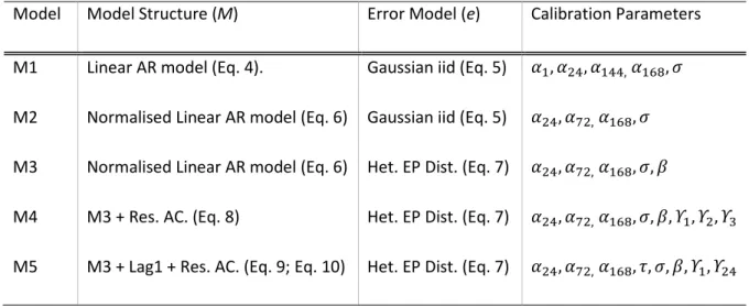
development are introduced, followed by a description of the calibration algorithm. Subsequently the iterative stages in model development from the initial model (M1) to the final model (M5) are described, as shown in Table 1. It is important to note that some additional models were tried at intervening iterations of the methodology – for the sake of brevity these have not been shown.
Table 1. Order of model development, model structure, error model and calibration parameters*
Model Model Structure (M) Error Model (e) Calibration Parameters
M1 Linear AR model (Eq. 4). Gaussian iid (Eq. 5) , !, !!, "#, $ M2 Normalised Linear AR model (Eq. 6) Gaussian iid (Eq. 5) !, % , "#, $ M3 Normalised Linear AR model (Eq. 6) Het. EP Dist. (Eq. 7) !, % , "#, $, &
M4 M3 + Res. AC. (Eq. 8) Het. EP Dist. (Eq. 7) !, % , "#, $, &, ', ', '( M5 M3 + Lag1 + Res. AC. (Eq. 9; Eq. 10) Het. EP Dist. (Eq. 7) !, % , "#, ), $, &, ', ' !
AR = Autoregressive; iid = independent, identically distributed errors; Het = Heteroscedastic model; EP = Exponential Power density function; Res = Residual; AC = Autocorrelation; *the numbered sub-scripts for calibration parameters represent the time lag in hours. See equations and text for a description of the model parameters.
4.1 Location and Data
The methodology is applied to forecast hourly water demand for three Yorkshire Water Services DMAs in the UK. The three DMAs are representative of many UK DMAs, have an average water consumption of 26.76 ls-1
(DMA1), 24.64 ls-1 (DMA2)and 6.57 ls-1 (DMA3) for the time period considered for each DMA. As an ensemble,
the DMAs cover light industrial, urban and rural regions. Each DMA has only one inlet, no outlets to other DMAs, and none have internal water storage. As the potential application of a demand forecasting model is to aid in the identification of abnormal conditions (e.g. pipe burst), the time-period of observations for each DMA were chosen to provide a set of data for model development and demand forecasting evaluation under normal demand conditions (e.g. actual water consumption plus background leakage). Therefore, obvious abnormal conditions were removed from the time-series, to provide a 271 day period for DMA1 (24/03/2011 to 20/12/2011), 230 day period for DMA2 (04/05/2011 to 20/12/2011) and for DMA3 a 224 day period (11/04/2011 to 21/11/2011) at an hourly time-step.
4.2 Model Calibration
Upon selection of a model structure the Differential Evolution Markov Chain (DEMC) algorithm was applied for global calibration of the model parameters; more details of which can be found in Ter Braak (2006). Briefly, a generation of *Markov chains are run in parallel to explore parameter space, following random initialisation from uniform prior distributions for each parameter. Wide uniform priors were set for each parameter based on exploratory time-series analysis of lag correlation and demand variability. Once the likelihood +| is evaluated for each chain, its location is updated using the Differential Evolution algorithm, which generates a proposal by adding to the location of the current chain the difference between the location of two other chains, multiplied by a factor ,, plus a random sample drawn from a small symmetric distribution. The proposal likelihood +|- is calculated, and the proposal accepted using the metropolis algorithm: if the ratio +|-/+| is greater than a random number on the interval [0, 1] then the proposal is accepted. During sampling , = 2.38/√22, where 2 is the number of parameters, and * = 22.Every 10th generation ,
is set to one to allow jumps between modes in parameter space. Following an initial burn in period, the simulation was stopped once the Gelman and Rubin (1992) convergence criterion dropped below 1.2 for all parameters.
4.3 Primary Model
The initial model M1 applied to all three DMAs is endogenous in structure in that past water demands up to the forecasting time are used as inputs to the forecasting model. Auto-correlation plots and visual inspection of the relationship between demand at time step t4 and lagged demand 456 were employed to identify initial time-lags ; hours for model input. Based on this analysis a linear auto-regressive model was initially applied for demand forecasting at time t in each DMA:
4 = 45+ !45 !+ !!45!!+ "#45"# 4
where is a multiplier for each lagged demand, and indicates the time-lag. Thus, 4 parameters in total were calibrated from the model. The residual errors are initially assumed to be independent and identically distributed according to a Gaussian likelihood function with zero mean and constant standard deviation $. Thus, this assumption for the residual errors results in a standard least squares approach. For convenience the log-likelihood is applied in calibration:
+| = −2 ln2π −2 ln$ − BC2σ− D 6
F
The model parameters in equation 4, alongside the error model standard deviation, are jointly calibrated using the DEMC algorithm on the first half of the dataset available for each DMA. The second half of each dataset is used for validation.
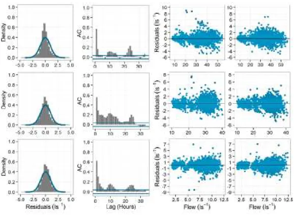
All three DMAs show similar calibration performance, as exemplified by the standardised residuals for each (Figure 2). The diagnostic plots show that the iid assumptions made in applying the Gaussian assumption for the residual errors are inappropriate: the true residual distributions are heavier tailed; significant autocorrelation occurs up to lags of 5 hours, and around 12 and 24 hours; and the residuals are also heteroscedastic with larger residuals errors at higher flow rates. The sharpness and reliability of the 95% prediction interval for M1 is shown in Figure 3 for all DMAs, plotted as a function of the time of day. The assumed coverage of the residuals by the prediction bounds under-estimates the actual percentage of observations that fall inside the bounds during the night time. During peak morning demand there is a large drop in reliability, as the prediction bounds fail to adequately cover the correct number of observations. Analysis of the residuals as a function of day of the year for each DMA (not shown) reveals that the largest residuals occur either on public holidays, or when one of the lagged demands used as input to the model falls on a public holiday. The effect of this contributes to the heavy tailed residual distributions that the Gaussian error model cannot adequately represent, and therefore an over-estimation of the model predictive uncertainty, particularly under normal working day conditions.
Figure 2. Standardised residuals (predictions minus observations) for DMA 1 (top row), DMA 2 (middle row) and DMA 3 (bottom row), plotted as a histogram alongside the assumed distribution (solid black line) derived from M1 (1st column);
residual autocorrelation with 95% significance levels (grey dashed lines; 2nd column); and residuals plotted as a function
of simulated flow (3rd column). The right hand column (4th Column) shows residuals plotted as a function of simulated
flow for model M2.
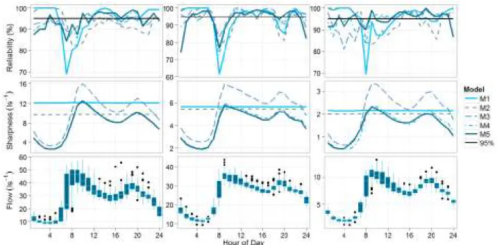
Figure 3. Percentage of observations covered by the 95% prediction bound during calibration (Reliability), compared to the theoretical coverage (black horizontal line at 95%); Sharpness of the 95% predictive distribution; box plots of observed flow variability. All graphs plotted as a function of the hour of the day for DMA 1 (left column), DMA 2(middle column) and DMA 3 (right column), derived from models M1 to M5.
4.4 Data Transformation
A number of approaches may be taken to deal with the negative effect of public holidays on demand forecasting in general, from removing them from the analysis (Amaral et al., 2008), modifying the model structure to account for different days of the week (Cutore et al., 2008), and data transformation. A data transformation is applied here, in a similar vein to Bakker et al. (2013), to normalise the effect of the day of the week on the data for all three DMAs. First, demand for each hour of each day was categorised into either a working day (weekdays excluding public holidays) and non-working day (weekend days and public holidays). A vector of normalised demands 6 were obtained by dividing demand for each hour of the day by a day factor: HI. The day factor equals the average demand for that hour of the day on the same day type (working or non-working day) in the preceding 15 days, divided by the average demand for that hour over all previous days in the 15 day window. Following normalisation for each DMA, the time-series were re-analysed as described in section 4.3 to identify the best optimal prediction lags. The lag 1 term was removed compared to
the model in equation 4 as the relationship showed significant scatter in comparison to the retained lags. Similar optimal lags were identified for all DMAs, resulting in the following model structure:
4 = HIJC ! 645 !+ % 645% + "# 645"#D 6
Thus the normalised demands are used in prediction, and multiplied by the day factor in order to obtain the predicted demand. The new model was calibrated using the same error model (Equation 5), using the same procedure presented in section 4.3. Data normalisation removed many of the larger residuals associated with public holidays, as shown in Figure 2. Figure 3 shows the reliability and sharpness of the 95% predictive distribution in calibration, compared to the discharge variability plotted as a function of the time of day. Data normalisation led to an improvement in the sharpness (e.g. reduction in the width) of the 95% predictive distribution, notably for DMA 1 (Figure 3). Even though the bounds became narrower, normalisation also led to an improvement in the reliability of the 95% prediction bound in comparison to M1. The bound for M2 is much closer to the theoretical coverage at 7am and 8am in all DMAs. The reason for improvement is that it is at these hours of the day that there is the greatest difference between bank holiday and weekday demand that led to the large residual errors in M1. This is likely associated with people who are more active earlier in the day before work. However, there is also a decline in reliability during the evening peak demand, and the error model still over-estimates predictive uncertainty at night-time, where the prediction bounds cover close to 100% of the observations. A homoscedastic error model assumes constant variance, and produces a predictive distribution of fixed width (sharpness) across the day (Figure 3). Such an error model fails to reflect the temporal variation in aleatory demand uncertainty, which is lowest at night, where there is little variability, and greatest during the day, particularly during the morning peak where demand is high. Heteroscedastic errors such as these may also result from measurement uncertainties. Such heteroscedasticity can also be seen in Figure 2.
Figure 4. Standardised residuals (predictions minus observations) for DMA 1 (top row), 2 (middle row) and 3 (bottom row) plotted as a histogram alongside the assumed distribution (solid black line) derived from M3; autocorrelation with 95% significance levels (grey lines); and residuals plotted as a function of simulated flow.
4.5 Residual Error Model Modification
In order to better represent the true distribution of residual errors, heteroscedasticity is introduced by assuming that the error standard deviation is a linear function of flow: $= $. In addition a kurtosis parameter & is introduced which results in an exponential power distribution and the following log-likelihood: +|L = − lnCMND − B ln$ 6 F − ONBP− σ P /QN 6 F 7
where MN and ON are derived from &, the kurtosis parameter (see Schoups and Vrugt, 2010), which is jointly inferred alongside the model parameters and $. The newly employed likelihood function applied with the model in Equation 6 (M3) leads to a much better representation of the heavier tailed residual distribution, and stabilises the heteroscedasticity for all DMAs, as shown in Figure 4. In predictive terms, the likelihood in equation 7 allows the sharpness of the model predictive distribution to vary across the day to much better reflect the true variance in demand (Figure 3). Despite a reduction in sharpness during the day, notably during
the morning and evening peaks, the 95% prediction bounds are now more reliable – e.g. the sharpness has to decline, notably during the morning peak, to better bracket the observations with the correct coverage. The negative effect of over-estimation of predictive uncertainty at night, and under-estimation during the day that resulted from applying Equation 5 has been reduced. In DMA 3, however, the reliability of the 95% prediction bounds has worsened at night, and the predictive bounds have become too sharp. Such sharpening suggests the simple linear relationship between discharge and error variance is inappropriate in this DMA. Figure 4 also shows that there is a strong Lag 1 autocorrelation in all DMAs.
4.6 Auto-correlation
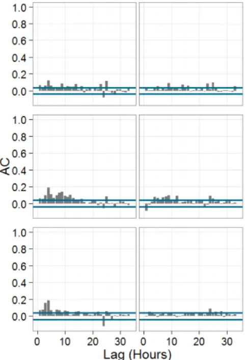
The autocorrelation suggests there are still components – or trends in the system - that need to be “whitened”, as the residual pattern is not random (Bennett et al., 2013). Therefore residual error autocorrelation terms, prior to normalisation, were added to the model in equation 6:
4 = HIJS ! 645 !+ % 645% + "# 645"#+ B '45
T
F U 8
where is the normalised residual error at lag , V is number of lags in included in the model, and ' is a calibrated parameter for each lag. For each DMA the model was recalibrated using the likelihood in Equation 7, resulting in model M4. The additional autocorrelation terms reduced the lag-1 residual error, most notably for DMA 3, as shown in Figure 5 where V was increased up to 3. However, the model was not completely able to remove lag 1 and lag 2 autocorrelation, particularly for DMA 1 and 2. The inclusion of autoregressive error terms led to an improvement in sharpness of the predictive distributions for all DMAs. In terms of robustness this led to a small decline in reliability of model M4 for DMA 1 for the first 9 hours of the day in comparison to M3, whereas for DMA 3 the same model modifications led to an improvement in night time reliability. In all DMAs the narrowing of predictive distribution led to a decline in reliability for peak morning demand. The inclusion of predictor variables in the model with shorter lags explains the general improvement in predictive performance with sharper bounds, with modest declines in reliability for the 95% prediction interval. Yet autocorrelation remains. As explained previously, the lag 1 term in Equation 6 was removed moving from M1 to M2 as despite a strong R2 between
64 and 645, there was a fair amount of scatter in the relationship.
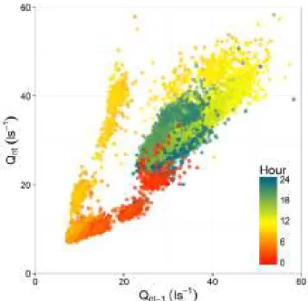
Further exploratory analysis of this relationship (Figure 6) shows that the scatter is not random, but rather the lag 1 gradient varies as a function of the time of day. As an alternative approach to deal with lag 1 autocorrelation, the lag 1 term is re-introduced in the model in normalised form:
4= HIJC ! 645 !+ % 645% + "# 645"#+ 645+ '45+ ' !45 !D 9
= ) 645 !
645 X 10
therefore the gradient of the lag 1 term is allowed to vary as a function of time of day by combining the calibration parameter ) with the equivalent gradient from the previous day. Initial model runs (not shown) showed that there was still some lag 1 correlation, and the introduction of the gradient term also introduced some lag 24 and lag 25 correlation. Therefore two additional residual error correlation terms were introduced (Equation 9), with associated calibration parameters ' and ' !. The resultant model, M5 removed the majority of the autocorrelation from the residuals for each DMA, and in this respect showed improvement in comparison to M4 (Figure 5). The effect of this change in the predictive performance of the model is very minor for DMA 1; for DMA 2 there is a slight worsening in sharpness and slight improvement in robustness for 7am; and for DMA 3 there is an overall improvement in robustness.
Figure 5. Autocorrelation plots with 95% significance levels (grey lines) for model M4 (top row) and M5 (bottom row) for DMA 1 (1st column), 2 (2nd column) and 3 (3rd column).
Figure 6. Normaliseddemand 64 plotted against normalised demand at lag 1 hour 645 for DMA 1. The colour of the points shows the time of day (hours).
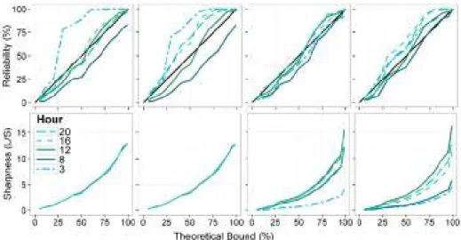
Figure 7 compares the sharpness and reliability of model M1 and M5 in both calibration and validation across a range predictive percentiles for 5 different hours of the day for DMA 1 (for the sake of brevity, results for all DMAs are not shown). Regardless of the model there is a decline in reliability moving from calibration to validation. In all DMAs M5 produces more reliable prediction bounds as the reliability curves for each hour of the day fall closer to the 1:1 line. The most notable improvement in performance occurred for DMA 3. Importantly the improvement in reliability is also accompanied by an improvement in sharpness of the prediction bounds, most notably at night (3am). The effect of this can be most clearly seen in Figure 8, which shows time-series plots of observed demand and predictive uncertainty. Model M5 produces prediction bounds that better reflect the time-varying nature of demand uncertainty across the day in comparison to those derived using a Gaussian model with constant heteroscedasticity. Furthermore, the prediction bounds are generally sharper across all hours of the day, which as shown in Figure 3 for the 95% prediction interval occurs once lag – 1 terms are re-introduced into the model in M4 and M5, in comparison to previous models.
Figure 7. Reliability (top row) and sharpness (bottom row) plots for model M1 in calibration (first column) and validation (second column), and for model M5 in calibration (third column) and validation (fourth column) for DMA 1 plotted for 5 different times of the day (24 Hour clock).
Figure 8: Time-series of observed demand (black bullets), 95% prediction intervals (width of shaded area), for DMA 1 modelled using M1 (top) and M5 (bottom). Shading from dark to light within the 95% prediction interval indicates narrower prediction bounds.
5.
Discussion
The assumption that the residual error distribution is adequately described by a Gaussian iid likelihood function was shown to be inappropriate for demand forecasting in the three DMAs considered in this case study. This finding has implications for the application of demand forecasting model calibration procedures
that employ mean square error based approaches that also make these assumptions. The residual error structures in this case study were characterised by heavier tails and heteroscedasticity – evidence for which has been found elsewhere (Bakker et al., 2013b; Alvisi et al., 2007). The diagnostic methodology aided in the identification of these errors, alongside other deficiencies in model performance (e.g. autocorrelation), and resulted in a model that uses a formal Bayesian likelihood function that account for kurtosis and heteroscedasticity in the residual distribution that better reflected the true nature of residual errors. Calibration using such approaches is required to prevent bias in parameter calibration that can result from inappropriate assumptions (Schoups and Vrugt, 2010). If information is available to quantify independently different sources of error, such as measurement error, then it may be preferable to quantify error sources independently (e.g. Kuczera et al 2006), as joint inference of model and error model parameters may then be avoided when updating error model structure. However, re-calibration at each stage of model development is efficient computationally with the models applied in this study. It is important to consider that diagnostic tests applied in this study may lead to the rejection of formal Bayesian approaches, particularly if epistemic errors are of greater importance (Beven et al., 2008; Hutton et al., 2013). However, this is entirely compatible with the iterative methodology presented here, and also recommended in the framework of Hutton et al (2014) for choosing an appropriate method for dealing with model uncertainty.
An adequate model of the residual errors is not just important for calibration, but also to provide an adequate description of model predictive uncertainty. In the presented methodology sharpness (width) and reliability (nominal coverage) are used as measures of the adequacy of the predictive distributions. The derived predictive distributions from model M5, which provides a better representation of the residual errors, are sharper, particularly at night time, than model M1. What is critically important is that the improvement in sharpness, and therefore confidence in the accuracy of the model prediction, has not come at the expense of a drop in reliability. Rather, the reliability of the model has also improved. In comparison to previous deterministic approaches, the result of the application of the proposed methodology is a richer set of information that more accurately quantifies the time-varying nature of demand uncertainty. Such information may be of particular use for differentiating between normal and abnormal conditions, as the range of normal demand behaviour has been quantified probabilistically for different times of the day. This is an area of ongoing research.
The performance of model M5 developed through the methodology can be compared tentatively, and only in an average sense to previous models, and for the three DMAs considered produced Mean Absolute Percentage Errors (MAPE) in calibration (and validation) for the 1 hour ahead forecasts of 5.07% (4.07%), 3.09 (4.09%) and 4.25% (3.85%) for DMA 1, 2 and 3, respectively, which are at the lower end of the range of errors previously reported in the literature, including for these DMAs (Romano and Kapelan, 2014). For DMA 1 and
DMA 3 there was a slight improvement in forecasting performance in validation, which likely reflects a decline in demand variability towards the latter half of the year, not least due to fewer bank holidays in the validation time-period.
The overall aim of the applied methodology was to obtain a useful model. Part of a model’s use in water distribution systems is real-time application, where computational resources limit model application. Thus whilst the developed methodology requires user interaction to identify and implement improvements in model performance, model terms are added (as with the transition from model M4 to M5), when justified by the data to derive parsimonious model structures that are better suited to real time application. Such models may be run in an ensemble in real-time to then quantify predictive uncertainty. An approach starting with simple models is also appropriate for situations where data available for calibration are scarcer, as may be the case in other water related fields. In such situations care should be taken to avoid poor parameter identifiability with addition of more parameters, which may be a particular issue in adequately characterising prediction uncertainty.
Alongside the detection of abnormal conditions, the greater level of information on predictive uncertainty may also be useful for control optimisation under normal conditions. Such modelling would require demand forecasts for up to 1-2 days. Further work will investigate the application of the methodology for deriving forecasting models to predict over a larger forecasting horizon. Whilst previous studies have generally identified a monotonic decline in forecasting accuracy as a function of lead time (Romano and Kapelan, 2014), it is expected, given the time-varying nature of demand uncertainty identified, that this will vary as a function of the time of model forecast (e.g. Alvisi et al., 2007). Additional diagnostic tests will therefore be required to evaluate and improve model performance.
6.
Conclusions
In order to better account for the aleatory and epistemic uncertainties that affect the performance of water demand forecasting, a probabilistic methodology is presented for quantifying, diagnosing and reducing model structural and predictive errors for the iterative development of short term water demand forecasting models. The application of the methodology revealed problems with calibration based on simplistic Gaussian iid assumptions, which in the case study considered led to inappropriate estimation of predictive uncertainty. The developed methodology emphasises iterative model development, calibration and testing using diagnostic checks of both the residual errors and frequentist properties of the predictive distributions. Application of the methodology led to development of a parsimonious model structure suitable for real-time modelling using a formal Bayesian likelihood function that accounts for kurtosis and heteroscedasticity in the
residuals. The model produced sharper yet still reliable predictive distributions that better quantify the time varying nature of demand uncertainty in water supply systems.
7.
References
Adamowski, J. F., 2008. Peak daily water demand forecast modeling using artificial neural networks. Journal of Water Resources Planning and Management, 134(2), 119-128.
Adamowski, J., Fung Chan, H., Prasher, S. O., Ozga-Zielinski, B., & Sliusarieva, A., 2012. Comparison of multiple linear and nonlinear regression, autoregressive integrated moving average, artificial neural network, and wavelet artificial neural network methods for urban water demand forecasting in Montreal, Canada. Water Resources Research, 48(1).
Almutaz, I., Ali, E., Khalid, Y., & Ajbar, A. H., 2013. A long-term forecast of water demand for a desalinated dependent city: case of Riyadh City in Saudi Arabia. Desalination and Water Treatment, (ahead-of-print), 1-8.
Alvisi, S., Franchini, M., & Marinelli, A., 2007. A short-term, pattern-based model for water-demand forecasting. Journal of Hydroinformatics, 9(1), 39-50.
Alvisi, S., & Franchini, M., 2010. Pipe roughness calibration in water distribution systems using grey numbers. Journal of Hydroinformatics, 12(4), 424-445.
Amaral, L.F., Souza, R.C., and Stevenson, M., 2008. A smooth transition periodic autoregressive (STPAR) model for short-term load forecasting. International Journal of Forecasting, 24: 603-615
Arbués, F., Garcıa-Valiñas, M. Á., & Martınez-Espiñeira, R., 2003. Estimation of residential water demand: a state-of-the-art review. The Journal of Socio-Economics, 32(1), 81-102.
Bakker, M., Vreeburg, J.H.G., Palmen, L.J., Sperber, V., Bakker, G., Rietveld, L.C., 2013a. Better water quality and higher energy efficiency by using model predictive flow control at water supply systems. Journal of Water Supply: Research and Technology, AQUA 62 (1), 1-13.
Bakker, M., Vreeburg, J. H. G., Van Schagen, K. M., & Rietveld, L. C., 2013b. A fully adaptive forecasting model for short-term drinking water demand.Environmental Modelling & Software, 48, 141-151.
Bennett, N. D., B. F. W. Croke, G. Guariso, J. H. A. Guillaume, S. H. Hamilton, A. J. Jakeman, S. Marsili- Libelli, L. T. H. Newham, J. P. Norton, C. Perrin, S. A. Pierce, B. Robson, R. Seppelt, A. A. Voinov, B. D. Fath and V. Andreassian, 2013. Characterising performance of environmental models."Environmental Modelling & Software 40: 1-20. DOI 10.1016/j.envsoft.2012.09.011.
Beven, K., 2008. On doing better hydrological science. Hydrological processes, 22(17), 3549-3553.
Beven, K., Smith, P. J., and Wood, A., 2011. On the colour and spin of epistemic error (and what we might do about it), Hydrology and Earth System Sciences Discussions, 8, 5355–5386, doi:10.5194/hessd-8-5355-2011 Box. G., 1976. Science and Statistics. Journal of the American Statistical Association. 71(356): 791-799
Breinholt, A., Møller, J. K., Madsen, H., & Mikkelsen, P. S., 2012. A formal statistical approach to representing uncertainty in rainfall–runoff modelling with focus on residual analysis and probabilistic output evaluation– Distinguishing simulation and prediction. Journal of Hydrology, 472, 36-52.
Cloke, H. L., & Pappenberger, F., 2009. Ensemble flood forecasting: a review.Journal of Hydrology, 375(3), 613-626.
Cutore, P., Campisano, A., Kapelan, Z., Modica, C., & Savic, D., 2008. Probabilistic prediction of urban water consumption using the SCEM-UA algorithm. Urban Water Journal, 5(2), 125-132.
Deletic, A., Dotto, C. B. S., McCarthy, D. T., Kleidorfer, M., Freni, G., Mannina, G., Uhl, M., Henrichs, M., Fletcher, T. D., Rauch, W., Bertrand-Krajewski, J. L. and Tait, S., 2012. Assessing uncertainties in urban drainage models, Physics and Chemistry of the Earth, Parts A/B/C, 42-44, 3-10.
Engeland, K., Xu, C. Y., & Gottschalk, L., 2005. Assessing uncertainties in a conceptual water balance model using Bayesian methodology/Estimation bayésienne des incertitudes au sein d’une modélisation conceptuelle de bilan hydrologique. Hydrological Sciences Journal, 50(1).
Gelman, A. and Rubin, D.B., 1992. Inference from iterative simulation using multiple sequences. Statistical Science, 7, 457–472.
Gelman, A. And Shalizi, C.R., 2012. Philosophy and Practice of Bayesian Statistics. British Journal of Mathematical and Statistical Psychology. 66: 8-38.
Ghiassi, M., Zimbra, D. K., & Saidane, H., 2008. Urban water demand forecasting with a dynamic artificial neural network model. Journal of Water Resources Planning and Management, 134(2), 138-146.
Gupta, H. V., Wagener, T., & Liu, Y., 2008. Reconciling theory with observations: Elements of a diagnostic approach to model evaluation.Hydrological Processes, 22(18), 3802-3813.
Herrera, M., Torgo, L., Izquierdo, J., & Pérez-García, R., 2010. Predictive models for forecasting hourly urban water demand. Journal of Hydrology, 387(1), 141-150.
Hutton, C., Kapelan, Z., Vamvakeridou-Lyroudia, L., and Savić, D., 2014. Dealing with Uncertainty in Water Distribution System Models: A Framework for Real-Time Modeling and Data Assimilation. J. Water Resour. Plann. Manage., 140(2), 169–183.
Hutton, C., Kapelan, Z., Vamvakeridou-Lyroudia, L., and Savić, D., 2013. The Application of Formal and Informal Bayesian Methods for Water Distribution Hydraulic Model Calibration. J. Water Resour. Plann. Manage., 10.1061/(ASCE)WR.1943-5452.0000412 (Oct. 3, 2013).
Kapelan, Z., Savic, D.A. and Walters, G.A., 2007. Calibration of WDS Hydraulic Models using the Bayesian Recursive Procedure, ASCE Journal of Hydraulic Engineering, 133(8), 927-936.
Kuczera, G., Kavetski, D., Franks, S. and Thyer, M., 2006. Towards a Bayesian total error analysis of conceptual rainfall-runoff models: Characterising model error using storm-dependent parameters. Journal of Hydrology 331(1-2): 161-177
Liu, Y., & Gupta, H. V., 2007. Uncertainty in hydrologic modeling: Toward an integrated data assimilation framework. Water Resources Research, 43(7).
Liu, Y., Freer, J., Beven, K., & Matgen, P., 2009. Towards a limits of acceptability approach to the calibration of hydrological models: Extending observation error. Journal of Hydrology, 367(1), 93-103.
Martinez, F., Hernandez, V., Alonso, J., Rao, Z., & Alvisi, S., 2007. Optimizing the operation of the Valencia water-distribution network. Journal of Hydroinformatics, 9(1), 65-78.
McMillan, H., & Clark, M., 2009. Rainfall-runoff model calibration using informal likelihood measures within a Markov chain Monte Carlo sampling scheme. Water Resources Research, 45(4).
Mounce, S., Boxall, J., and Machell, J., 2010. ”Development and Verification of an Online Artificial Intelligence System for Detection of Bursts and Other Abnormal Flows.” J. Water Resour. Plann. Manage., 136(3), 309– 318.
Qi, C., & Chang, N. B., 2011. System dynamics modeling for municipal water demand estimation in an urban region under uncertain economic impacts. Journal of environmental management, 92(6), 1628-1641.
Romano, M. and Kapelan, Z. 2014. Adaptvie Water Demand Forecasting for Near Real-Time Management of Smart Water Distribution Systems, Journal of Environmental Modelling and Software, 60, 265-276.
Schoups, G., Vrugt, J.A., 2010. A formal likelihood function for parameter and predictive inference of hydrologic models with correlated, heteroscedastic, and non-Gaussian errors. Water Resources Research 46, W10531. http://dx.doi.org/10.1029/2009WR008933.
Ter Braak, C. J., 2006. A Markov Chain Monte Carlo version of the genetic algorithm Differential Evolution: easy Bayesian computing for real parameter spaces. Statistics and Computing, 16(3), 239-249.
Vrugt, J. A., Ter Braak, C. J. F., Diks, C. G. H., Robinson, B. A., Hyman, J. M., & Higdon, D., 2009. Accelerating Markov chain Monte Carlo simulation by differential evolution with self-adaptive randomized subspace sampling.International Journal of Nonlinear Sciences and Numerical Simulation, 10(3), 273-290.
Zhou, S.L., McMahon, T.A., Walton, A., Lewis, J., 2002. Forecasting operational demand for an urban water supply zone. Journal of Hydrology 259, 189–202.