United States Department of Agriculture
Forest Service
Pacific Southwest Forest and Range Experiment Station
General Technical Report PSW-38
a user's guide to Probit Or LOgit analysis
Authors:
JACQUELINE ROBERTSON is a research entomologist assigned to the
Station's insecticide evaluation research unit, at Berkeley, Calif. She earned a B.A. degree (1969) in zoology, and a Ph.D. degree (1973) in entomology at the University of California. Berkeley. She has been a member of the Station's research staff since 1966. ROBERT M. RUSSELL has been a computer programmer at the Station since 1965. He was graduated from Graceland College in 1953, and holds a B.S. (1956) degree in mathematics from the University of Michigan. N.E. SAVIN earned a B.A. degree (1956) in economics and M.A. (1960) and Ph.D. (1969) degrees in economic statistics at the University of California, Berkeley. Since 1976, he has been a fellow and lecturer with the Faculty of Economics and Politics at Trinity College, Cambridge University, England.
Acknowledgments:
We thank Benjamin Spada, Pacific Southwest Forest and Range Experiment Station, Forest Service, U.S. Department of Agriculture, Berkeley, California; and Drs. William O'Regan and Robert L. Lyon, both formerly with the Station staff, for providing valuable encouragement and criticism during the time POLO was written. We also thank Dr. M.W. Stock, University of Idaho, Moscow; Dr. David Stock, Washington State University, Pullman; Dr. John C. Nord, Southeast Forest Experi-ment Station, Forest Service, U.S. DepartExperi-ment of Agriculture, Athens, Georgia; and Drs. Michael I. Haverty and Carroll B. Williams, Pacific Southwest Forest and Range Experiment Station for their suggestions regarding this guide.
Publisher
Pacific Southwest Forest and Range Experiment Station P.O. Box 245, Berkeley, California 94701
POLO:
a user's guide to Probit Or LOgit analysis
Jacqueline L. Robertson Robert M. Russell N. E. Savin
CONTENTS
Introduction . . . 1
1. Statistical Features . . . . 1
2. Aspects of Bioassay Design . . . . 2
2.1 Selection of Test Subjects . . . 2
2.2 Sample Size . . . 2
2.3 Dosage Selection . . . 3
2.4 Control Groups . . . 3
2.5 Replication . . . 3
3. Data Input Format . . . . 4
3.1 Starter Cards . . . 4
3.2 Header Cards . . . 4
3.3 Preparation Cards . . . 4
3.4 Dosage-Response Cards . . . 4
3.5 Control Group Cards . . . 5
3.6 Metameter . . . 5
3.7 Command Cards . . . 6
3.8 Sample Input for Standard Probit Analysis . . . 7
4. Data Output Format . . . 8
4.1 Data Printback . . . 8
4.2 Metameter Listing . . . 8
4.3 Analysis Message . . . 8
4.4 Individual Preparation Printout . . . 8
4.5 Likelihood Ratio Test of Equality . . . 9
4.6 Likelihood Ratio Test of Parallelism . . . 10
4.7 Summaries . . . 10
1Walton, Gerald S. Unpublished program for probit analysis.
Copy of program on file at the Pacific Southwest Forest and Range Experiment Station, Forest Service, U.S. Department of Agriculture, Berkeley. California.
POLO
(Probit Or LOgit) is a computer program specifically developed to analyze data obtained from insecticide bioassays. Prior to its development, other computer programs by Daum (1970), Daum and Killcreas (1966), and Walton1 were used for that purpose. After using these programs extensively, we concluded that they were neither sufficiently accurate for our needs, nor did they produce the output we desired.The statistical procedures incorporated into POLO, its documentation, and examples of its application are described in articles by Robertson and others (1978a, b), Russell and others (1977), Russell and Robertson (1979), and Savin and others (1977). Copies of these articles may be obtained upon request to:
Director
Pacific Southwest Forest and Range Experiment Station P.O. Box 245
Berkeley, California 94701 Attention: Publication Distribution
The POLO program is also available upon request. A magnetic tape with format instructions should be sent to the above address, attention: Computer
Services Librarian. The program is currently operational on the Univac 1100 Series, but can be modified for other large scientific computers.
This guide was prepared to assist users of the POLO program. Statistical features of the pro-gram, suggestions for the design of experiments that provide data for analysis, and data input and output formats are described in detail.
1. STATISTICAL FEATURES
POLO performs the computations for probit or logit analysis with grouped data. For a discussion of these methods, see, for example, the text by D. J. Finney (1971). In contrast to previous programs, the computational procedure has been completely freed from dependence on traditional manual methods and is entirely computer-oriented.
The statistical basis for POLO is a binary quantal response model with only one independent variable in addition to the constant term. Consider subjects placed in one of T possible experimental settings, where each setting requires one of two possible responses from the subject. For example, in a bio-assay in which insects are treated with one of T doses of a chemical insecticide, the possible responses are
dead or alive. There is a measured characteristic of the test subjects for each experimental setting. We denote a numerical function of the measured characteristic for the t-th setting by zt. In the bioassay example, the measured characteristic is the dose; the numerical function zt may be the dose, the logarithm of the dose, or some other function of the dose.
The model analyzed is Pt = F(
α
+β
zt), where F is a cumulative distribution function (CDF) mapping the points on the real line into the unit interval. For the probit modelPt = F(
α
+β
zt) =Φ
(α
+β
zt)where Φ is the standard normal CDF. For the logit model
Pt = F(
α
+β
zt) = 1/[1 + e-(α +βt)]Both models are estimated by the method of maxi-mum likelihood.
Beyond the traditional computations, POLO tests hypotheses involving two or more regression lines. When several chemical preparations are com-pared, a probit or logit regression line is calculated independently for each preparation. Two hypotheses are tested next. The first hypothesis is that all regression lines are equal, that is, that all have the same intercept and the same slope. The second hypothesis is that all lines are parallel, that is, all have the same slope. Both hypotheses are tested by means of the likelihood ratio test.
The standard normal and logistic CDF's are quite close to one another except in the extreme tails. Therefore, similar results are obtained with either model unless data comes from the extreme tails of the distribution. For theoretical and empirical rea-sons for using these functions, other sources should be consulted (Berkson 1951, Cox 1966, Finney 1971).
2. ASPECTS OF BIOASSAY
DESIGN
POLO output is only as good as the data input. Program output is the basis for valid statistical inference about the probit or logit model, provided that an appropriate experimental design has been employed in the data collection process. In the following discussion, we consider aspects of experi-mental design of insecticide bioassays. With suitable generalization, the same considerations pertain to many other binary quantal response bioassays, such as those with drugs or plant growth regulators.
2.1 Selection of Test Subjects
The population of test subjects should be care-fully defined before the bioassay is performed. Once a population—for example, larvae in a particular developmental stage—has been defined, the test sub-jects should be randomly selected in order to eliminate bias in the experimental results.
To ensure randomization, it is advisable to use a random number table or some other randomization device. Suppose, for example, that an insecticide is to be applied to last stage lepidopterous larvae within a particular weight range. The population, therefore, is composed of all insects in the last instar whose weight lies within the designated limits. Con-sider 75 rearing containers holding appropriate test subjects. One randomization procedure consists of numbering the containers from 1 to 75. For one day's test, five containers will provide sufficient test subjects; these five are selected by choosing the containers corresponding to the first five digits of a list of random numbers from 1 to 75. For the next day's test, containers matching the next five digits of the random number list may be used. This proce-dure may be repeated until all of the insects needed have been selected, assuming that insects in the original 75 containers remain within the weight limits.
During a given day's test, insects are frequently grouped with others for treatment. For example, a bioassay may be conducted with larvae held in petri dishes in groups :of. 10. Nine dose levels will be applied to the larvae held in 18 dishes. One way to randomize dosage assignments would be to number the petri dishes as they are filled. Using a random number table, the investigator may then assign the dishes corresponding to the first two digits of a random number table to dose level A, the second two to dose level B, and so on.
These randomization procedures work well, given a relatively unlimited supply of test subjects such as that provided by a continuous laboratory culture. When wild populations are tested, some modifications of randomization procedures may be necessary. For example, natural units such ascones may be numbered, then selected at random for assignment to bioassays with each of a group of insecticides. These randomization techniques are not the only ones which an investigator may follow; however, we have found them useful in our routine bioassays. Instructions for using random number tables are available in statistical textbooks (Gold-stein 1964, Snedecor and Cochran 1967).
2.2 Sample Size
The maximum likelihood estimates and likeli-hood ratio tests used in POLO have desirable large
3 sample properties. There appears to be no firm
guideline regarding the sample size (that is, number of test subjects) which must be used for these desira-ble properties to hold. Typically, we have used 300 to 500 insects for each bioassay of a particular chemical performed with test subjects selected from a laboratory colony.
When insects are obtained from field collections, their numbers are frequently limited. Even when the number of test subjects is not limited, the time available for a bioassay may be a limiting factor. In general, we have found that treatment of more insects with fewer compounds is preferable to treat-ment of fewer insects with more compounds. This procedure tends to maximize the number of test subjects treated with a single chemical.
2.3 Dosage Selection
A preliminary dose-fixing experiment is a useful step in the selection of the test dosages to be applied in a bioassay. In this procedure, a small number of test subjects is used to test the effects of a wide range of dosages. Suppose, for example, that insecticide A is to be tested for the first time on a target insect species. We suggest that a logarithmic series of dilu-tions from 0.001 to 10.0 mg/ ml be tested, with each concentration applied to 10 insects at the usual volume or rate. The complete series of dosages in this experiment would be 0 (controls treated with solvent only), 0.001, 0.01, 0.10, 1.0, 10.0 (mg/ ml). The resultant percentage mortalities might be: control―0; 0.001―0; 0.01―0; 0.10―30; 1.0―100; 10.0―100. These data would serve as a guide for dosage selection for the main bioassay.
More precise estimates of the probit and logit lines are obtained when some dosages are placed in the tails of the tolerance distribution and some are placed in the middle, rather than clustering all dosages in the middle. When only five dosages are used, 95 percent confidence limits for the lethal dosages cannot be computed about 25 percent of the time due to the high values of g (see p. 9). Therefore, we recommend that eight or more dosages be used to estimate any regression by means of POLO. From the results of the dose-fixing experiment described above, we would use the following dosages in the first replication of the main experi-ment (mg/ ml): 0.05, 0.07, 0.10, 0.20, 0.30, 0.50, 0.70, and 1.0.
After the first replication, a further adjustment of dosages can be made. Suppose the results of the first replication of our hypothetical bioassay were (per-cent mortality): control―0; 0.05―0; 0.07―5; 0.10―20; 0.20―35; 0.30―43; 0.50―52; 0.70―80; 1.0―90. For the second replication, it would be wise to omit the 0.05 mg; ml dosage and add one of
2.0 mg/ ml. Ideally, a range of mortalities from about 5 percent to about 95 percent should result from treatment with dosages finally selected.
2.4 Control Groups
A control group should be included in any bio-assay. In our insecticide bioassay example, the con-trol is considered to be a dose level of 0 mg/ ml. The rationale for control groups is self-evident. Without them, an investigator can never be certain that lethal effects are wholly attributable to the insecticide being tested. The solvent or an impurity in the solvent may have been toxic to the test subjects.
Excess test subjects should not be used as the control group. The controls must represent a random sample selected from the population by the same criteria and procedures used to assign test subjects to any other dose group. Preferably, each test chemical should have its own control; an alternative, but less desirable, design uses a com-bined control consisting of all control groups from all chemicals tested in a particular experiment. Using either type of control data, POLO will calculate a theoretical control response ("natural response") for each chemical on an individual basis. The program will also calculate response lines without controls; in this instance, the program assumes that control mortality is zero. Unless the investigator has reason to assume that control mortality is in fact zero, this option is not recommended.
POLO calculates a theoretical response rate of untreated test subjects―the "natural response." It should be emphasized that natural response and control group mortality are not the same. Natural response is a theoretical rate based on the pattern of responses exhibited at all dose levels. The zero and lowest dosages, however, carry more weight in the calculations. Control group mortality is the re-sponse rate actually observed in the control group; random variation may cause it to differ somewhat from the theoretical rate.
2.5 Replication
A bioassay should be replicated (that is, repeated several times) in order to randomize effects related to laboratory procedure, such as worker or day effects. Suppose that chemical A is to be tested on a population of insects from a laboratory colony. The supply of test subjects is plentiful, so that a mini-mum of three replications can be performed.
Obvious differences between the results of one replication and another suggest that laboratory pro-cedures, such as formulation or application
tech-nique, should be investigated. In our hypothetical bioassay, the first replication of applications of chemical A killed 5 to 95 percent of the test subjects, but all test subjects were killed by all dosages in the second replication. The purpose of the next replica-tion should then be to trace whether a procedural error had occurred in either of the two preceding replications.
3. DATA INPUT FORMAT
3.1 Starter Cards
Every POLO run starts with five cards which call the program from a tape (fig. 1):
Cards 2-5 must be punched as shown. Some modi-fication of card 1 is possible. Columns 9-23 identify a particular work unit and account number which can be changed to identify the particular user. Column 26 is the time limit, 28-30 the page limit. Time and page limits can be changed to suit the user's particular needs. In most cases, 2 minutes and 200 pages far exceed what is necessary for an analysis.
The fifth starter card can be modified slightly for very restricted use (fig. 2). In some of the bioassays for which POLO was designed, dosages must be multiplied by 10 to appear in the conventional units usually reported. Specifically, dosages in topical application bioassays of insecticides are applied at the rate of μg/ 100 mg body weight; they are reported in units of μg /g body weight. Substitution of a card reading
for starter card 5 multiplies lethal dosages reported in the last summary printed by the program by 10. The dosages printed in the body of the output are not converted. This input format option is available for special circumstances only.
By using the starter format (fig. 1), units reported in the summary and body of POLO output will be the same as units in the data input.
3.2 Header Cards
Each group of data sets starts with a header card with an equal sign (=) punched in column 1. Any-thing desired can be punched on the rest of the card. The computer merely prints everything on the header card, so any information useful for identify-ing the data sets should be entered (fig. 3):
Figure 3
There can be any number of header cards introduc-ing the data sets.
3.3 Preparation Cards
Each data set is composed of the dose-response data. Each separate group (insecticide, generation, treatment method) is called a preparation and is identified by an asterisk (*) in column 1. The name of the preparation should start in column 2. The computer retains only the first eight characters and uses them to label the printout. If a name or group title exceeds eight characters, it is wise to abbreviate the titles so that separate groups are identified. For example, carbaryl has been tested in two different formulations, S.4.0 and S.L. If the following prepa-ration cards (fig. 4) were used, the computer would identify each group with the same label (CARBARYL):
However, preparation cards using abbreviations would identify each preparation clearly (fig. 5):
3.4 Dosage-Response Cards
One card per dose group should be punched. POLO will analyze one to 300 dose groups for each preparation. Each dose-response card contains three fields, punched in order. The first field is dose, the second is number of subjects, the third is number responding (for example, dead). The num-ber in each field need not appear in particular columns. Only one or more spaces need separate the fields. If each preparation has its own control group, it should be entered as a dose-group with dose level
5 zero. The order of the dosage-response cards does
not matter (figs. 6 and 7). Analyses of both data sets in these examples would be identical.
No firm rationale exists for definition of dose groups. In figures6 and 7, data for four replications (dose-fixing and main experiment) of the experi-ment have been combined. Another, perhaps pref-erable, procedure is to list data for each replication separately (figure 8). This procedure tends to minimize test statistics such as HET (p. 9) and g (p.
9) by increasing the number of degrees of freedom used in the linear regression calculations.
3.5 Control Group Cards
As noted above, individual control groups for each preparation are entered as a dose-group with a dose level of zero. POLO will calculate probit or logit lines without control groups; however, ifone preparation has a control group, all other prepara-tions must also have a control. We recommend an experimental design in which each test group or preparation has its own control group. If, however, the experimental design is such that a single control group applies to all of the preparations, the joint control group should be entered as if it were an additional preparation with one dose group. The preparation card is *NATURAL and the dose group card contains the dosage (0), the number of subjects, and the number responding (fig. 9):
3.6 Metameter
If doses are not to be converted to logarithms by POLO, a D-card should be entered following the dose-response data (fig. 10):
The D-card has a D punched in column 1, followed by one or more spaces, then the number 1. Suppose, for example, that dosages were converted to loga-rithms during the summarization of dosage-response data. Dosages might then be listed on the dosage-response cards as follows (fig. 11):
Further conversion of the dosages would result in logarithms of logarithms; therefore, the D-card should be used to ensure that the dosages would be used as is. This option is called the "arithmetic" metameter.
3.7 Command Cards
If command cards are not used, POLO's standard calculations will be performed. These consist of calculations of individual probit lines for each preparation, the likelihood ratio test for equality among all preparations listed behind each header card, and the likelihood ratio test of parallelism of the preparations. Other options can be selected by use of command cards.
3.7.1 C-Card
The first command card is a C-card, which contains a C in column 1 and up to three numbers following. The C and the numbers must be sepa-rated from one another by blank spaces. If only a C is punched in column 1, the card is equivalent to a C followed by three zeroes. This is, in turn, equivalent to no card at all, and results in the standard output. Thus, the standard output will result from:
• No command card
• A card with C in column 1 (fig. 12):
• A card with C in column 1 and three zeroes, with the zeroes separated from the C and each other by a space (fig. 13):
If a one is substituted for the first zero, logit analysis will be performed (fig. 14):
If a one is substituted for the second zero, the natural response parameter will not be estimated by maximum likelihood (ML). In figure 15, logit analysis without estimation of natural response is to be performed; in figure 16, probit analysis without estimation of natural response is commanded:
Finally, the substitution of a one for the last zero affects the interpretation of the next command card, the P-card (see sec. 3.7.3). If the last number is zero, the entries on the P-card are merely starting values to aid the computer in its search for the optimum, or maximum likelihood, value. If a one is entered, the values on the P-card are to be considered final and no search will be undertaken by the computer. The figures below illustrate all possible combinations:
Figure 17A specifies logit analysis, with estimation of natural response and a computer search for maxi-mum likelihood values of other parameters. Figure 17B specifies logit analysis without estimation of natural response, but with a computer search for ML values of other parameters. Figure 17C commands logit analysis without estimation of natural response; specified values of the other parameters are designated by the P-card to follow. Finally, figure 17D commands logit analysis, estimation of natural response, but values of other parameters will be specified by the P-card.
The command cards for probit analysis are shown in figures 17E to H. Figure 17E commands probit analysis, estimation of natural response, and ML search for other parameters (STANDARD OPTION). Figure 17F designates probit analysis without estimation of natural response, but with ML search for other parameters. Figure 17G commands probit analysis, estimation of natural response, but values of the other parameters will be specified by the P-card. Finally, figure 17H commands probit analysis without ML estimation of natural response, and with values of other parameters specified by the P-card.
3.7.2 L-Card
The second command card, the L-card, specifies the percentages for which lethal dosages (LD's), will be calculated. These percentages are integers from 1 to 99. As many as 12 percent levels may be listed. At least one space should separate the numbers (fig. 18):
The L-card in figure18 will result in printing of LD5, 10, 15, 35, 50, 60, 65, 75, 80, 90, 95 and 99 in the output. Omitting the L-card results in printing of the stand-ard LD's—LD10, LD50, LD90.
3.7.3 P-Card
The last command card, the P-card, should be used only under unusual circumstances. It allows the user to specify starting values of the parameters. In most instances, these might be estimates of ML values to help POLO maximize the likelihood func-
7 tion. For this use, the C-card must have a zero
punched as the last of the three numbers.
When a one is punched as the third entry on the C-card, the values on the P-card will be used as fixed parameters; the program will not search for a sup-posedly more optimal set.
3.7.4 Cautions
If any command card is present, the C-card must also be present even if it is empty. Those command cards present must be in the order C, L, P.
A group of command cards produces a single type of analysis of the data. These may be followed by other command cards which will produce a different analysis of the same data.
Following the command cards, another data set may be entered. This would consist of the header card(s) distinguished by an equal sign (=) in column 1, dose-response data, and, perhaps, command cards. To the computer, this is an entirely new batch of data bearing no relationship to those preceding or any following.
3.7.5 Options: An Example
In the following example of the use of command cards for multiple analyses of the same data, two preparations have been tested (fig. 19). Natural response will be estimated as a parameter. The data first will be analyzed using probits; the analysis will then be repeated using logits. There is a joint control group valid for both preparations. The only LD to be printed is the LD50.
3.8 Sample Input for Standard
Probit Analysis
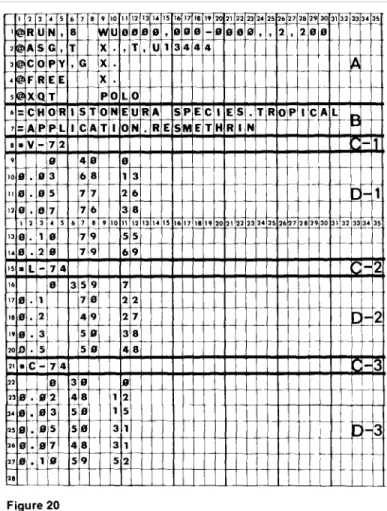
Figure 20 illustrates a typical input for probit analysis. All of the card groups—starter, header, preparation, and dosage-response—are illustrated.
The starter cards are in group A, the header cards are in group B. Card C-1 is the preparation card for the first data set; card C-2, the preparation for the second set; card C-3 the preparation card for the third set. The preparation data sets themselves are contained on card sets D-1, D-2, and D-3. To obtain standard logit analyses, rather than probit analyses, of the same data sets, a C-card specifying the logit transformation (fig. 14) must follow each data set (D-1, D-2, and D-3).
The output from this set of sample data is dis-cussed in detail in section 5. Briefly, an analysis of each data set, the likelihood ratio test for equality of the three sets, and the likelihood ratio test for paral-lelism will be printed. If the user is interested in pair comparisons, each pair must run separately behind a separate header card (fig. 21). For large numbers of pair comparisons (for example, those for all pos-sible combinations of two from a group of 15 prepa-rations) a computer storage system may be used.
The elements (preparations) can then be recalled as needed for the various pair comparisons.
4. DATA OUTPUT FORMAT
In this section, the format of data output from POLO (fig. 22), will be described in detail. A sample output, resulting from the input shown in figure 20, is presented in its entirety. Probit analysis is per-formed; the format for logit analysis is identical.
4.1 Data Printback
All cards for preparations following each header card are printed back prior to the statistical analysis (fig. 22A). After the analysis for one group is com-pleted, the next group following the next header card is printed, then analyzed. This printback fea-ture provides an opportunity for rechecking the accuracy of the data input.
4.2 Metameter Listing
The next section of the data output (fig. 22B) lists each preparation, dose, dose-metameter transfor-
mation, subjects, responses, and decimal propor-tion of responses. The number or preparapropor-tions and number of dose-response cards follows the metame-ter listing.
4.3 Analysis Message
Following the metameter list, POLO prints a message specifying the analysis conducted. (fig. 22C). The user is told which transformation will be used for the analysis, whether natural response is a parameter, and whether the program will estimate parameters by maximum likelihood.
4.4 Individual Preparation
Printout
Terminology in the printouts for individual prepa-rations is derived from Finney (1971). When the user is unsure of statistical meanings or derivations of terminology, Finney's text should be consulted. Use of likelihood ratio tests in the context of probit and logit analyses is discussed by Savin and others (1977).
The top of each page repeats the first header card (line 1, secs. D1, D2, and D3).2 Next, the constraints of the analysis are stated together with the preparation title (line 2, secs. D1, D2, D3). For individual preparations, intercepts and slopes are always unconstrained. The analyses are simply regressions of each dose metameter on response, with correction for natural response where appro-priate. Note that the position of each preparation in the group is specified by the numeral immediately preceding the preparation title in line 2. In the third line of the individual analyses (line 3, secs. D1, D2, D3), POLO states whether or not it will estimate natural response as a parameter. In sections D1 and D3, no response was observed in either control group; it follows, therefore, that the program will operate by "not estimating natural response." In section D2, on the other hand, the program will be "estimating natural response" because mortality was observed in the control.
In the fourth line of the printout, the logarithm of the maximum value of the likelihood function for each preparation is presented (line 4, secs. D1, D2, D3). In the next section (lines 5-7, secs. D1, D3; lines 5-8, sec. D2), values of the intercept (α, labeled with the preparation title), slope, and natural response (where appropriate) are listed in the column called "parameter." The standard errors and t-ratios
2For purposes of easier reference, section and line divisions are
cited on the following pages which relate specifically to the computer printout in figure 22.
(parameter value ÷ standard error) of each para-meter are listed in the succeeding columns.
The variance-covariance matrix of the parameters is listed next (lines 8-11, secs. D1, D3; lines 9-13, sec. D2), followed by the chi-squared goodness-of-fit test (lines 12-18, secs. D1, D3; lines 15-20, sec. D2) The chi-square value, degrees of freedom, and heterogeneity factor (which equals the chi-square divided by the degrees of freedom) follow (line 19, secs. D1, D3; line 21, sec. D2). When the heterogeneity factor exceeds 1.00, the user is cautioned by a warning (lines 22-24, sec. D2; lines 20-22, sec. D3). The program suggests that a plot of the data be consulted, since the model fits the data poorly. Although random variation (that usually termed "experimental error") may account for a large chi-square (and heterogeneity), a plot of the data may reveal systematic variation from linear regression. In this eventuality, use of a different mathematical function may be more appropriate for analyzing the data. In most cases, we have found that variation in insecticide bioassays cannot be clas-sified as systematic; nevertheless, the user has been warned of a problem with the data and is free to decide what, if anything, to do about it,
The "index of significance for potency estima-tion" (line 20, sec. D1; line 25, sec. D2; line 23, sec. D3) is the statistic g which is used for calcula-tion of confidence limits at three probability levels-90, 95, and 99. If, at any of these levels, g exceeds 1.00, the values of the mean may lie outside the limits; for very large values of g, the confidence limits run from -∞ to +∞ (Finney 1971). As a safety feature, POLO calculates confidence limits only when g is less than 0.5 at either the 90, 95, or 99 percent probability levels. A warning about g is printed (lines 26-27, sec. D2; lines 24-25, sec. D3) when g at any of the three probability levels is over 0.5. Should this occur, a statement (line 28, sec. D2; line 26, sec. D3) of the maximum value of g which the program will accept is made. Note that the value of g is less than 0.5 at all three probability levels in section D1; no warning statement appears, and 90, 95 and 99 percent confidence limits have been calculated (lines 21-25, last 6 columns). In sections D2 and D3, however, g exceeds 0.5 at the 99 percent probability level; the user is given the g warning and only 90 and 95 percent confidence limits are calculated (last four columns each of lines 29-33, sec. D2 and lines 27-31, sec. D3).
Calculated effective doses (lethal doses or lethal concentrations, depending on the test technique) are the final portion of each printout (lines 21-25, sec. D1; lines 29-33, sec. D2; lines 27-31, sec. D3). In the first column, the dose level of percent effect is labeled. The standard option lists LD10, LD50, and LD90. In the next column, the preparation name is reprinted. The column labeled DOSE lists the
calculated dosage required for the specified percent effect. In figure 22, the LD10's, LD50's and LD90's are:
. Preparation LD50 LD50 LD90 . V-72 0.02159 0.06852 0.21753 L-74 0.05913 0.16239 0.44596 C-74 0.01329 0.04139 0.12892
4.5 Likelihood Ratio Test of
Equality
Section E is the portion of the POLO printout for the likelihood ratio test of equality of the three individual preparations shown in sections D1, D2, and D3. The header card message is printed first (sec. E, line 1), followed by a description of the statistical hypothesis tested (line 2). The test of equality constrains the slopes and intercepts to be the same. With these constraints, the lines would be the same. Natural response is not estimated in determining the composite line (3) for comparison.
Lines 4-11 contain the statistics for the composite lines and are analogous to those for the individual preparations (lines 4-11, secs. D1, D3; lines 4-13, sec. D2). The most important calculation listed is the logarithm of the maximum value of the likeli-hood function for the composite line (line 4, sec. E). The next section presents the likelihood ratio test for equality itself (lines 12-14, sec. E). To determine whether the lines are equal, the program is "testing the hypothesis that slopes and intercepts are the same" (line 12, sec. E). The negative of twice the value of the difference of the sum of the likelihood functions of the individual preparations and the likelihood function of the composite line is distributed as a chi-square (line 13, sec. E). The degrees of freedom (d.f.) (line 13, sec. E) equals the number of parameters for each line (=2), multiplied by the number of lines (in this example, 3) minus the number of parameters constrained in the composite line (slope + intercept, =2). Thus, d.f. equals (2 × 3) -2, or 4 in the present example. POLO then calcu-lates the probability corresponding to the chi-square with the proper degrees of freedom (line 13, sec. E). If the probability is greater than 0.05, the hypothesis is accepted; if the probability is less than 0.05, the hypothesis is rejected. In this example, the hypothesis is rejected (line 14, sec. E).
In the remaining portion of the printout, the same information previously presented for individual lines (preparations)—the chi-squared goodness-of-fit statistic, heterogeneity, g, effective dosages, their limits, and appropriate warnings—is listed for the composite line (lines 15-43, sec. E). The user need not be concerned with large values of chi-squared, heterogeneity factors, or g values which commonly appear for composite lines. If lines are grossly unequal, these statistics will become quite large.
4.6 Likelihood Ratio Test of
Parallelism
The likelihood ratio test for parallelism (sec. F) follows the test for equality. Once again, the header title is printed (line 1, sec. F). The statistical hypothesis to be tested follows. For the test of paral-lelism, the slopes of the individual preparation lines are constrained to be the same (line 2, sec. F). Natu-ral response is not estimated (line 3, sec. F).
The logarithm of the likelihood function for the composite line generated when the slopes of the preparations are constrained to be the same is calcu-lated next (line 4, sec. F). The intercepts for the individual preparations with slopes constrained (lines 6-8, sec. F) and the slope of the composite line (line 9, sec. F), standard errors of the parameters and t-ratios for each line are printed. The variance-covariance matrix is also listed (lines 10-15, sec. F). The likelihood ratio test for parallelism (lines 16-18, sec. F) is presented in the same format described for the test of equality. Degrees of free-dom, (d.f) for the test equals the number of preparations (three) times the number of param-eters constrained (one:the slope), minus the number of constrained parameters in the composite line (one:the slope). In this example, d.f. = (3 × 1) - 1 = 2. As in the test for equality, the hypothesis is accepted when the tail probability is greater than 0.05. In the present example, the hypothesis is accepted.
The statistics for the chi-squared goodness-of-fit test of the combined line and the calculation of g are shown in lines 19-36, section F. These precede the calculations of effective doses and confidence limits for the individual preparations (lines 37-50, sec. F) assuming the same slope as the composite line. Finally, the potency of each preparation relative to the first preparation in the group (lines 51-55, sec. F) is calculated according to the procedures of Finney (1971, p. 100-124).
4.7 Summaries
The first summary printed by POLO (fig. 22) is a guide to the body of the analysis and a synopsis of pertinent information. The header card title is first printed (line 1, sec. G). Then, key statistics for each preparation are listed (lines 2-13, sec. G). The first line lists the preparation title, number of subjects treated, number of controls, and the page number on which the detailed analysis for the preparation is to be found (lines 2, 8, 14, sec. G). In the next line, the log of the likelihood function, slope ± standard error, and natural response ± standard error are listed (lines 3, 9, 15, sec. G). Heterogeneity and the value of g at the 95 percent level follow (lines 4, 10,
16, sec. G). The next three lines give LD10, LD50, and LD90 values with their respective 95 percent confidence limits (lines 5-7, 11-13, 17-19, sec. G). The last two groups summarize the likelihood ratio tests for equality and parallelism (line 20-26, 27-33, sec. G). The statistics for each composite line with the appropriate constraints are printed as they were for individual preparations. If the value of g exceeds 0.5 at the 95 percent level, no list of LD values will appear in the summary. The user should refer to the analysis for possible reasons.
The second summary (sec. H) was designed for immediate assessment of results and photo reduc-tion. The columns are:
Abbreviation . Data presented . PREP Preparation
N Number of test subjects
NC Number of controls
C, SE Estimated natural response ± its standard error
BETA, SE Slope ± its standard error LD50, Calculated lethal dose for 50 per-95% limits cent effect and 95 percent
dence limits of that dose LD90, Calculated lethal dose for 90 per-95% limits cent effect and 95 percent
dence limits of that dose
HET Heterogeneity factor (chi squared ÷ degrees of freedom)
G g at the 95 percent probability level LOG L Logarithm of the maximum value of
the likelihood function HYP OK indicates whether either
hypo-thesis tested (equality or paral-lelism) is accepted (p> 0.05)
4.8 Error Messages
Error messages clearly indicate mistakes in the data input:
Message Reason The data on this card seems
to be out of order. The number responding on a dosage-response card is greater than the number of test subjects. The usual reason is transposing of the numbers when either writing the data forms or punching the cards. If one preparation has a
control group, all prepara-tions must have a control
Self-explanatory group.
EUREKA Your data are so outlandish that no analysis can be performed. Try again.
Figure 22―Data output from POLO is shown in printouts.
LITERATURE CITED
Berkson, J.
1951. Why I prefer logits to probits. Biometrics 7:327-339.
Cox, D, R.
1966. Some procedures connected with the logistic qualitative response curve. In Research papers in statistics, p.
51-71. F. N. David, ed. John Wiley and Sons, London. Daum, R, J.
1970. A revision of two computer programs for probit analysis. Bull. Entomol. Soc. Amer. 16(1):10-l5.
Daum, R. J., and W. Killcreas.
1966. Two computer programs for probit analysis. Bull. Entomol, Soc. Amer. 12(4):365-369.
Finney, D. J.
1971. Probit analysis. 3d ed., Cambridge University Press, London and New York.
Goldstein, A.
1964. Biostatistics. Macmillan Publishing Co., Inc., New York.
Robertson, J. L., L. M. Boelter, R. M. Russell, and N. E. Savin. 1978. Variation in response to insecticides by Douglas-fir
tussock moth, Orygia pseudotsugata (Lepidoptera: Lymantriidae) populations. Can. Entomol. 110:325-328.
Robertson, J. L., N. L. Gillette, B. A. Lucas. R. M. Russell, and N, E. Savin.
1978. Comparative toxicity of insecticides to Choristoneura species (Lepidoptera: Tortricidae). Can. Entomol. 110: 399-406.
Russell, R. M., and J. L. Robertson.
1979. Programming probit analysis. Bull. Entomol, Soc.
Amer, 25(3):191-192.
Russell, R. M., J. L. Robertson, and N. E. Savin.
1977. POLO: A new computer program for probit analysis.
Bull. Entomol. Soc. Amer. 23(3):209-213. Savin, N. E., J. L. Robertson, and R. M. Russell.
1977. A critical evaluation of bioassay in insecticide re-search: likelihood ratio tests of dose-mortality regres-sion. Bull. Entomol. Soc. Amer. 23(4):257-266.
Snedecor, G. W., and W. G. Cochran.
1967. Statistical methods. 6th ed. Iowa State University
Press, Ames, Iowa.
Robertson, Jacqueline L., Robert M. Russell, and N. E. Savin.
1980. POLO: a user's guide to Probit Or LOgit analysis. Gen. Tech. Rep. PSW-38,
15 p., illus. Pacific Southwest Forest and Range Exp. Stn., Forest Serv., U.S. Dep. Agric., Berkeley, Calif.
This user's guide provides detailed instructions for the use of POLO (Probit Or LOgit), a computer program for the analysis of quantal response data such as that obtained from insecticide bioassays by the techniques of probit or logit analysis. Dosage-response lines may be compared for parallelism or equality by means of likelihood ratio tests. Statistical features of the program, suggestions for the design of experiments that provide data for analysis, and formats for data input and output are described in detail.