Entropy-copula method for single-site monthly streamflow simulation

Entropy-copula method for single-site monthly streamflow

simulation

Z. Hao1and V. P. Singh1,2

Received 18 September 2011; revised 26 April 2012; accepted 2 May 2012; published 13 June 2012.

[1] An entropy-copula method is proposed for single-site monthly streamflow simulation.

In this method, the joint distribution of adjacent monthly streamflows is constructed using the copula method, whereas the marginal distribution of streamflow for each month is derived using the entropy method. Then, the conditional distribution is derived from which monthly streamflow is generated. Moment statistics of monthly streamflow (such as mean, standard deviation and skewness) can be modeled by the entropy-based marginal

distribution while the dependence structure between streamflows of adjacent months can be modeled by the copula-based joint distribution. The proposed entropy-copula method can be extended by incorporating an aggregate variable for modeling the interannual

dependence. Application to the simulation of monthly streamflow from the Colorado River illustrates the effectiveness of the proposed method.

Citation: Hao, Z., and V. P. Singh (2012), Entropy-copula method for single-site monthly streamflow simulation,Water Resour. Res., 48, W06604, doi:10.1029/2011WR011419.

1. Introduction

[2] Synthetic streamflow data are needed in water resources studies for the evaluation of alternative designs and policies against the range of sequences that are likely to occur in the future [Loucks et al., 1981]. It is desired that synthetic streamflow is similar to historical streamflow and preserves moment statistics (such as mean, standard devia-tion, and skewness) and dependence structure (such as lag-one correlation). The interannual dependence is important for the simulation of long wet and dry periods [Sivakumar and Berndtsson, 2010], and also needs to be preserved. Sivakumar and Berndtsson [2010] provided a review of streamflow simulation models.

[3] The copula method has been extensively applied for hydrologic modeling mainly due to its flexibility in con-structing the joint distribution to describe the dependence structure between random variables. One of the most com-mon applications is frequency analysis of hydrological var-iables [Favre et al., 2004 ; Salvadori and De Michele, 2004 ; Genest et al., 2007 ; Kao and Govindaraju, 2008 ; Chebana and Ouarda, 2009 ; Salvadori and De Michele, 2010 ; Renard, 2011 ; Vandenberghe et al., 2011]. Recent years have been witnessing an upsurge in applications of the copula method. Bardossy and Li [2008] introduced a copula-based model to describe spatial variability for the

interpolation of groundwater quality parameters.Serinaldi [2009] employed the bivariate copula-based mixed distri-bution to deduce the multisite Markov model for modeling and generating daily rainfall series.Chowdhary and Singh [2010] developed a copula-based approach for reducing uncertainty in the parameter estimation of frequency distri-butions.Gyasi-Agyei[2011] used a copula to model the de-pendence structure of daily rainfall properties for daily rainfall disaggregation.

[4] One of the important applications of entropy theory is to derive the maximum entropy-based distribution of ran-dom variables [Kapur, 1989 ; Kesavan and Kapur, 1992]. Hao and Singh[2011] proposed the entropy method for sin-gle-site monthly streamflow simulation with the entropy-based joint distribution andLee and Salas[2011] proposed the copula method for annual streamflow simulation with the copula-based joint distribution. This study proposes an entropy-copula method for monthly streamflow simulation in which the joint distribution is constructed using the cop-ula method with the marginal distribution derived using the entropy method. The entropy-copula method is simpler than the previous work byHao and Singh[2011], since less pa-rameters are determined simultaneously and is able to model different (nonlinear) dependence structures of streamflow due to the copula component. To model the interannual de-pendence of monthly streamflow, an aggregate variable is used to guide the simulation. The proposed method is applied to the monthly streamflow of the Colorado River at Lees Ferry, Arizona, and its performance is evaluated by comparing generated and observed statistics.

2. Methodology

2.1. Entropy Theory and Marginal Distribution

[5] For a continuous random variableXwith probability density function (PDF) f(x) defined on the interval [a,b], 1_{Department of Biological and Agricultural Engineering, Texas A&M}

University, College Station, Texas, USA. 2

Department of Civil and Environmental Engineering, Texas A&M University, College Station, Texas, USA.

Corresponding author : Z. Hao, Department of Biological and Agricul-tural Engineering, Texas A&M University, College Station, TX 77843-2117, USA. ([email protected])

©2012. American Geophysical Union. All Rights Reserved. 0043-1397/12/2011WR011419

the Shannon entropy I can be expressed as [Shannon, 1948] : I¼ Zb a fðxÞlnfðxÞdx: (1)

[6] Using the principle of maximum entropy proposed byJaynes[1957] with the first four moments as constraints specified as :

Zb a

giðxÞfðxÞdx¼EðgiÞi¼0;1;. . .;4: (2)

[7] The maximum entropy-based PDF can be obtained as [Kesavan and Kapur, 1992] :

fðxÞ ¼exp½01x2x23x34x4; (3)

wherei,i¼0,1 ,. . ., 4, are the Lagrange multipliers ; and E(gi) is the expectation of the function gi(x) (gi(x) ¼ xi). The Lagrange multipliers in equation (3) can be determined in terms of the specified constraints using the Newton-Raphson method [Hao and Singh, 2011].

[8] The constraints in the form of moments have been used to derive the maximum entropy distribution of random variables in different areas [Mead and Papanicolaou, 1984; Smith, 1993; Gotovac et al., 2010]. In addition, the distribu-tion in equadistribu-tion (3) can also model bimodality in the data [Matz, 1978]. For streamflow simulation, the distribution derived from the entropy method in equation (3) can be used as the marginal distribution of streamflow for each month and samples drawn from the distribution can be expected to pre-serve the mean, standard deviation, skewness (and kurtosis).

[9] The cumulative distribution function (CDF) of the maximum entropy-based PDF in equation (3) can be expressed as

EXðxÞ ¼ Z x

a

fðtÞdt: (4)

2.2. Copula Theory and Joint Distribution

[10] For the continuous random vector (X,Y)with mar-ginal CDFsFX(x) andFY(y), the joint distribution function of the random vector (X,Y) can be expressed with its mar-ginal CDFs and copulaCas [Nelsen, 2006] :

PðXx;Y yÞ ¼C½FXðxÞ;FYðyÞ; ¼Cðu;v;Þ; (5)

whereis the parameter of the copula that measures the de-pendence between marginals ; and uandvare realizations of the random variables U ¼ FX(x) and V ¼FY(y). The two-dimensional CopulaCmaps the two marginal distribu-tions into the joint distribution as [0,1]2! [0,1]. For the estimation of parameter, the method of moment (MOM), the exact maximum likelihood (EML) method, and the in-ference functions for margins (IFM) method can be used [Joe, 1997 ;Genest and Favre, 2007].

[11] There are several copula families and a variety of dependence structures can be modeled [Joe, 1997 ; Nelsen, 2006]. For example, random variables from both

the Gaussian copula and Frank copula exhibit symmetric dependence, while those from the Clayton copula exhibit asymmetric dependence [Trivedi and Zimmer, 2005]. For streamflow simulation, the joint distribution of streamflows for two adjacent months constructed from the copula method in equation (5) can be used to model the (nonlinear) dependence structure of monthly streamflow.

[12] The conditional distribution of random variable Y givenX(denoted as C2j1(vju)) can be derived from the joint distribution in equation (5) as :

PðY yjX¼xÞ ¼C2j1ðvjuÞ ¼

@Cðu;v;Þ

@u : (6)

2.3. Entropy-Copula Method

[13] The proposed entropy-copula method combines the entropy method to derive the marginal distribution and the copula method to construct the joint distribution. The joint distribution from the entropy-copula method can be con-structed from equations (4) and (5) and expressed as :

PðX x;Y yÞ ¼C½EXðx;Þ; EYðy;Þ;; (7)

where and are the parameters of the entropy-based marginal distribution, and is the copula parameter. The IFM method can be used for parameter estimation, in which parameters of the marginal distributions and those of the copula can be split. Parameters and can be estimated by the Newton-Raphson method, while copula parameter can be estimated using the maximum likelihood method. Compared with the entropy based method proposed byHao and Singh [2011], less number of parameters needs to be estimated simultaneously. In addition, the copula compo-nent in the joint distribution enables the characterization of different (nonlinear) dependence structures [Joe, 1997 ; Nelsen, 2006].

[14] The samples from the joint distribution in equation (7) can be expected to preserve the mean, standard devia-tion, skewness through the entropy-based marginal distribu-tion and dependence structure through the copula-based joint distribution. The conditional distribution from the joint distribution in equation (7) can also be expressed using equation (6). Monthly streamflow can be generated sequen-tially from the conditional distribution and totally 12 condi-tional distributions have to be used.

2.4. Extended Entropy-Copula Method

[15] The proposed entropy-copula method can be extended to preserve the interannual dependence by introducing an ag-gregate variable in the conditional distribution similar to the framework developed by Sharma and O’Neill [2002]. For monthly streamflow denoted asX1,X2,. . .,X12,X13, X14,. . ., Xn, whereX1,X2,. . .,X12are the monthly streamflows of the first year and so on, an aggregated variable can be defined as the summation of the previous m monthly streamflows (m¼12 in this study) :

Zt1¼ Xm

i¼1

Xtj: (8)

[16] Denoting streamflows of two adjacent months as

with the cumulative distribution functions F(Xt1), F(Xt) andG(Zt1), respectively, the joint distribution of random vector (Zt1,Xt1,Xt) can be expressed by copulaCas :

PðZt1zt1;Xt1xt1;XtxtÞ ¼Cðv1;v2;v3;’Þ; (9)

where ’ is the parameter that can be a scalar or vector depending on the copula family;v1,v2, andv3are the real-izations of random variables V1 ¼ G(Zt1),V2¼ F(Xt1) andV3¼F(Xt). Then the conditional distribution ofXtgiven Xt1 and Zt1 (denoted as C3j12(v3jv1,v2)) can be derived from the joint distribution by copulaCin equation (9) as:

PðXtxtjZt1¼zt1;Xt1¼xt1Þ ¼C_3j12ðv3jv1;v2Þ ¼ @C2_ðv1;v2;v 3;Þ @v1@v2 @C2_ðv1;v 2;Þ @v1@v2 1_: (10)

[17] The procedure for generating monthly streamflow by the extended entropy-copula method is summarized as follows :

[18] 1. Pick any zt1and the corresponding xt1values from the historic record. Compute the corresponding cumula-tive probabilitiesGt1(zt1) (denoted asv1) andFt1(xt1) (denoted asv2).

[19] 2. Generate a uniform random number between [0, 1], which is considered to be the conditional cumulative probability corresponding to a specific valuext, given the ini-tial valuezt1and xt1(or v1 andv2). From equation (10), one obtains:C_3j12ðv3jv1;v2Þ ¼. The cumulative probability

Ft(xt) (denoted asv3) can be obtained as: v3¼C3j121ðÞand thenxtcan be obtained as:xt¼Ftðv3Þ.

[20] 3. Increase time step t and update random values

xt1andzt1.

[21] 4. Repeat steps (1)–(3) until the required length of monthly streamflow is generated (The first few streamflow values can be discarded to avoid initialization bias). 3. Application

[22] Monthly streamflow from the Colorado River at Lees Ferry, Arizona, from 1906–2003 was used for applica-tion of the proposed method. More details about the datasets are given by Hao and Singh [2011]. 100 flow sequences with 100 years of streamflow in each sequence were gener-ated to assess the performance of the proposed method. The basic statistics (mean, standard deviation, skewness, lag-one (Pearson) correlation, maximum and minimum values) and interannual dependence from generated streamflow were compared with those from the observed streamflow using box plots. The performance was considered to be satisfac-tory when a statistic fell in the box plot.

3.1. Marginal and Joint PDF

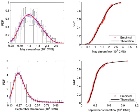
[23] Maximum entropy-based marginal PDF and CDF for each month were compared with empirical histograms and empirical CDFs estimated from the Gringorten plotting position formula. These results for the May and September streamflow are given in Figure 1. Generally the theoretical PDF fitted the empirical histogram relatively well and theo-retical CDF also fitted the empirical CDF well. Note that the skewness of September streamflow is relatively high

Figure 1. Comparison of empirical and theoretical PDFs and CDFs for the May and September stream-flow (Units for streamstream-flow are in Cubic Meter per Second (CMS)).

(1.96). These results showed that the entropy-based mar-ginal distribution modeled the underlying streamflow well, even though high skewness was involved. The bimodality in the PDF of the May streamflow, which has been found in the previous study [Prairie et al., 2006], was not resolved with the PDF in equation (3). However, this can be over-come when more moments are used to derive the entropy-based marginal distribution. To avoid the uncertainty in the estimation of higher moments from the historical record (98 years), the entropy-based PDF in equation (3) was used as the marginal distribution for monthly streamflow throughout the year. Box plots of the entropy-based mar-ginal PDFs for the generated May and September stream-flows are also shown in Figure 1, which shows the uncertainty of the moments estimated from the generated se-ries of a particular length (100 years) appreciably affects the entropy-based PDF in equation (3). Compared with the PDF estimated from the observed streamflow, the generated streamflow preserved the marginal distribution relatively well and the use of the first four moments as constraints to derive the marginal distribution is acceptable for this study.

[24] The Clayton, Frank, Gumbel and Gaussian copula functions were selected to construct the joint distribution. Two goodness of fit test statistics, the Crame´r–von Mises statistic (Sn) and Kolmogorov-Smirnov statistic (Tn) given byGenest et al.[2006], were employed to choose the suita-ble copula function. Statistics (Sn andTn) and the associ-ated p values based on a run of 5000 samples were obtained using the parametric bootstrap procedure [Genest et al., 2006 ;Genest and Favre, 2007]. Results for statistic Snare given in Table 1. The very lowpvalue (<0.05) sig-nified that the null hypothesis that the copula function was a valid model should be rejected. The times of streamflow pairs of adjacent months that a copula function was rejected for the Clayton, Frank, Gumbel and Gaussian copulas were 6, 4, 7, and 2, respectively. Similar results were also obtained from statistic Tn (times of rejecting the copula were 6, 2, 4, and 2, respectively). It can be seen that there was not a single copula function that performed best for modeling all streamflow pairs. A practical way for the simu-lation of monthly streamflow may be to choose different copula functions in modeling different streamflow pairs. The Gaussian copula function seemed to be preferable based on the number of rejections. In this study, the Gaussian copula function was selected hereinafter for the illustration of the proposed method for monthly streamflow simulation. The entropy-copula (EC) method and extended entropy-copula (EEC) method with the Gaussian copula function were denoted as ECG method and EECG method.

3.2. Basic Statistics

[25] A plot of observed monthly streamflow and a sequence of generated monthly streamflow for 98 years by the ECG method is shown in Figure 2. Generally the variabil-ity of generated streamflow was similar to that of observed streamflow (e.g., maximum and minimum values). Similar results were obtained from the streamflow generated by the EECG method (not shown).

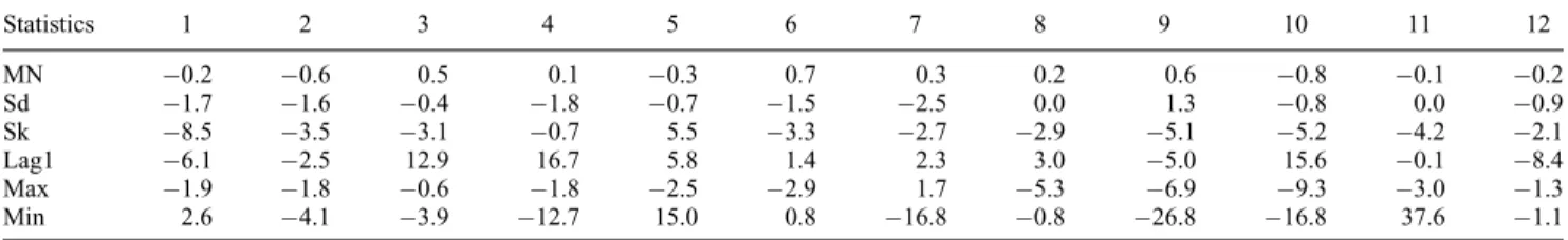
[26] Basic statistics of observed and generated streamflow by the ECG method are shown with box plots in Figure 3. The relative error (RE), defined as RE ¼ (Sm – Xo)/Xo, where Sm is the median of generated statistic andXois the observed statistic, for each statistic is shown in Table 2. The ECG method performed well in preserving the mean, stand-ard deviation, and skewness, since all the statistics fell in the box plot. The RE for mean and standard deviation was under 5% and that for skewness was under 10% for all months. In addition, there seemed to be some underestimation of stand-ard deviation and skewness for this simulation, since nega-tive relanega-tive error was obtained for 9 and 11 months, respectively.

[27] Generally the lag-one correlation was preserved well, though for certain months (e.g., October with RE of 15.6%) the observed statistic did not fall in the box. Com-pared with the entropy method by Hao and Singh [2011] using the same datasets, there seemed to be no significant difference in the preservation of mean, standard deviation and skewness between the two methods, while the entropy method performed relatively better than the entropy-copula method in preserving the lag-one correlation. However, when the Spearman and Kendall (rank) correlations were also used for measuring the dependence structure, results from the entropy-copula method, as shown in Figure 4, pre-served the two correlations well, while the entropy method did not preserve as well (not shown). These results showed the outperformance of entropy-copula method in preserving the nonlinear dependence. The maximum and minimum values were generally preserved well for most months (with RE under 5% and 20% for maximum and minimum values for most months), though overestimation or under-estimation for certain months occurred. Results of the EECG method in preserving these statistics of each month were similar to those by the ECG method and thus are not presented.

[28] Statistics of observed and generated streamflow at the annual time scale by the ECG and EECG methods are shown in Figure 5. The mean and standard deviation were preserved well by both methods. Neither ECG nor EECG method preserved the skewness well. The reason may be

Table 1. StatisticsSnand AssociatedpValues of Different Copulas for Different Streamflow Pairs

Copula SnandpValue 1–2 2–3 3–4 4–5 5–6 6–7 7–8 8–9 9–10 10–11 11–12 12–1

Clayton Sn 0.25 0.19 0.09 0.06 0.13 0.11 0.15 0.44 0.17 0.22 0.29 0.15 Clayton pvalue 0.01 0.05 0.32 0.65 0.13 0.09 0.03 0.00 0.04 0.01 0.00 0.10 Frank Sn 0.05 0.08 0.33 0.25 0.06 0.07 0.08 0.12 0.11 0.07 0.13 0.15 Frank pvalue 0.72 0.31 0.00 0.00 0.45 0.16 0.13 0.05 0.07 0.30 0.03 0.01 Gumbel Sn 0.06 0.22 0.51 0.54 0.21 0.14 0.19 0.11 0.16 0.08 0.06 0.10 Gumbel pvalue 0.64 0.02 0.00 0.00 0.01 0.01 0.00 0.15 0.04 0.30 0.52 0.13 Gaussian Sn 0.06 0.12 0.22 0.30 0.04 0.04 0.07 0.14 0.08 0.03 0.08 0.08 Gaussian pvalue 0.69 0.15 0.01 0.00 0.83 0.62 0.24 0.06 0.35 0.94 0.24 0.24

that simulation errors from both the mean and standard deviation would affect the simulated skewness. However, the two methods differed significantly in preserving the lag-one correlation. The EECG method preserved the lag-lag-one

correlation well, while the ECG method did not perform as well. The reason was that the lag-one correlation of annual streamflow was not incorporated in the ECG model, while for the EECG model this property was incorporated through

Figure 2. Comparison of observed monthly streamflow (98 years) and a sequence of generated monthly streamflow by the ECG method.

Figure 3. Box plots of basic statistics of observed and generated monthly streamflow by the ECG method. Continuous lines with star marks for each month represent statistics of historical record. Mn, Sd, Sk, Lag-1, Max and Min represent the mean, standard deviation, skewness, lag-1 correlation, maxi-mum and minimaxi-mum values.

the aggregate variable. For the preservation of maximum and minimum values, the ECG and EECG methods per-formed relatively well with slight overestimation.

3.3. Interannual Dependence

[29] The interannual dependence between streamflows of seasonal and annual time scales was also assessed for the EECG method. Box plots of lag-one and lag-four interan-nual dependence between streamflow of a specific month (seasonal time scale) and streamflows of the previous 12 months (annual time scale) of the generated streamflow are shown in Figure 6. It is seen that the lag-one correlation was preserved well for all months except for February, as expected from the structure of the EECG method. The lag-four correlation, although not directly included in the model, was also preserved well for most months.

4. Summary and Conclusion

[30] An entropy-copula method is proposed for single-site monthly streamflow simulation and is shown to preserve statistics of monthly streamflow well. The entropy-based

marginal distribution with the first four moments as con-straints is capable of modeling the complex properties (such as high skewness) of the underlying streamflow data. The mean and standard deviation of the generated streamflow at the annual time scale can also be preserved well. The extended entropy-copula method is shown to preserve inter-annual dependence well. The preservation of the lag-one correlation at the annual scale can also be improved by the extended method. However, the skewness at the annual time scale is generally not preserved well for both methods.

[31] Compared with the entropy method, the proposed entropy-copula method is easier to carry out in terms of pa-rameter estimation and enables the characterization of non-linear dependence structures due to the copula component. The use of higher moments (3rd and fourth moments in this study) as constraints to derive the marginal distribution relies on the accurate estimation of higher moments. Thus the proposed method is preferable for streamflow simula-tion with relatively long observasimula-tion record.

[32] The entropy method provides a way to derive the marginal distribution of hydrologic variables, including

Table 2. Relative Error (%) of Generated Statistics for Each Montha

Statistics 1 2 3 4 5 6 7 8 9 10 11 12 MN 0.2 0.6 0.5 0.1 0.3 0.7 0.3 0.2 0.6 0.8 0.1 0.2 Sd 1.7 1.6 0.4 1.8 0.7 1.5 2.5 0.0 1.3 0.8 0.0 0.9 Sk 8.5 3.5 3.1 0.7 5.5 3.3 2.7 2.9 5.1 5.2 4.2 2.1 Lag1 6.1 2.5 12.9 16.7 5.8 1.4 2.3 3.0 5.0 15.6 0.1 8.4 Max 1.9 1.8 0.6 1.8 2.5 2.9 1.7 5.3 6.9 9.3 3.0 1.3 Min 2.6 4.1 3.9 12.7 15.0 0.8 16.8 0.8 26.8 16.8 37.6 1.1 a

Mn, mean; Sd, standard deviation; Sk, skewness; Lag1, lag-one correlation; Max, maximum values; and Min, minimum values.

Figure 4. Box plots of Spearman and Kendall correlations of observed and generated monthly stream-flow by the ECG method.

Figure 5. Box plots of basic statistics of observed and generated annual streamflow by the (a) ECG method and (b) EECG method. Units for Mn, Sd, Max and Min are in 103CMS.

Figure 6. Box plots of lag-one and lag-four interannual dependence of observed and generated monthly streamflow by the EECG method.

some abnormal properties. For instance, to model multimo-dal property, the entropy-based distribution with moments as constraints provides an alternative way to resolve this property. The copula method offers the flexibility to model different (nonlinear) dependence structures of hydrologic variables through a variety of copula families. A combina-tion of these two theories, entropy and copula, enables the modeling of complex properties of the marginal distribu-tion and different dependence structures of data under investigation. One possible limitation of the entropy-copula method is that many Lagrange multipliers may be needed to derive the marginal distribution for modeling certain properties (e.g., multimode in the distribution) of the data. For the cases where a large number of Lagrange multipliers are involved in the entropy-based marginal distribution, the inference functions for margins (IFM) method for parame-ter estimation would reduce the burden of computational complexity. In addition, a potential limitation of the entropy-based marginal distribution would be that the desired prop-erty needs to be expressed in the form of constraints in order to derive the suitable marginal distribution. The connection between the properties (such as extreme values) of the data under investigation with the form of constraints needs fur-ther study.

[33] The entropy-copula framework can be applied and extended to higher dimensions for hydrologic modeling with the entropy-based marginal distribution to model the marginal properties and the copula-based joint distribution to model the dependence structure of the data. For certain hydrologic application (e.g., rainfall simulation), the copula method has made its way for practical use. With the entropy-based mar-ginal distribution, the entropy-copula framework would also be applicable as a complement to the current study.

References

Bardossy, A., and J. Li (2008), Geostatistical interpolation using copulas,

Water Resour. Res.,44, W07412, doi :10.1029/2007WR006115. Chebana, F., and T. B. M. J. Ouarda (2009), Index flood-based multivariate

re-gional frequency analysis,Water Resour. Res.,45, W10435, doi:10.1029/ 2008WR007490.

Chowdhary, H., and V. P. Singh (2010), Reducing uncertainty in estimates of frequency distribution parameters using composite likelihood approach and copula-based bivariate distributions,Water Resour. Res.,

46, W11516, doi :10.1029/2009WR008490.

Favre, A. C., S. El Adlouni, L. Perreault, N. Thie´monge, and B. Bobe´e (2004), Multivariate hydrological frequency analysis using copulas,

Water Resour. Res.,40, W01101, doi :10.1029/2003WR002456. Genest, C., and A. C. Favre (2007), Everything you always wanted to know

about copula modeling but were afraid to ask,J. Hydrol. Eng.,12(4), 347–368.

Genest, C., J. F. Quessy, and B. Re´millard (2006), Goodness of fit proce-dures for Copula models based on the probability integral transformation,

Scand. J. Stat.,33(2), 337–366.

Genest, C., A. C. Favre, J. Be´liveau, and C. Jacques (2007), Metaelliptical copulas and their use in frequency analysis of multivariate hydrological data,Water Resour. Res.,43, W09401, doi :10.1029/2006WR005275. Gotovac, H., V. Cvetkovic, and R. Andricevic (2010), Significance of

higher moments for complete characterization of the travel time proba-bility density function in heterogeneous porous media using the maxi-mum entropy principle,Water Resour. Res.,46, W05502, doi :10.1029/ 2009WR008220.

Gyasi-Agyei, Y. (2011), Copula-based daily rainfall disaggregation model,

Water Resour. Res.,47, W07535, doi :10.1029/2011WR010519. Hao, Z., and V. Singh (2011), Single-site monthly streamflow simulation

using entropy theory,Water Resour. Res.,47, W09528, doi:10.1029/ 2010WR010208.

Jaynes, E. (1957), Information theory and statistical mechanics,Physical Review,106(4), 620–630.

Joe, H. (1997),Multivariate Models and Dependence Concepts, Chapman and Hall, London.

Kao, S. C., and R. S. Govindaraju (2008), Trivariate statistical analysis of extreme rainfall events via the Plackett family of copulas,Water Resour. Res.,44, W02415, doi :10.1029/2007WR006261.

Kapur, J. (1989),Maximum-entropy Models in Science and Engineering, John Wiley and Sons, New York.

Kesavan, H., and J. Kapur (1992),Entropy Optimization Principles with Applications, Academic Press, New York.

Lee, T., and J. D. Salas (2011), Copula-based stochastic simulation of hydro-logical data applied to Nile River flows,Hydrol. Res.,42(4), 318–330. Loucks, D., J. Stedinger, and D. Haith (1981),Water Resource Systems

Planning and Analysis, Prentice-Hall, Englewood Cliffs, N.J.

Matz, A. (1978), Maximum likelihood parameter estimation for the quartic exponential distribution,Technometrics,20(4), 475–484.

Mead, L., and N. Papanicolaou (1984), Maximum entropy in the problem of moments,J. Math. Phys,25(8), 2404–2417.

Nelsen, R. B. (2006),An Introduction to Copulas, Springer, New York. Prairie, J., B. Rajagopalan, T. Fulp, and E. Zagona (2006), Modified K-NN

model for stochastic streamflow simulation,J. Hydrol. Eng.,11(4), 371–378. Renard, B. (2011), A Bayesian hierarchical approach to regional frequency analysis,Water Resour. Res.,47, W11513, doi:10.1029/2010WR010089. Salvadori, G., and C. De Michele (2004), Frequency analysis via copulas: Theoretical aspects and applications to hydrological events, Water Resour. Res.,40, W12511, doi :10.1029/2004WR003133.

Salvadori, G., and C. De Michele (2010), Multivariate multiparameter extreme value models and return periods : A copula approach,Water Resour. Res.,46, W10501, doi :10.1029/2009WR009040.

Serinaldi, F. (2009), A multisite daily rainfall generator driven by bivariate copula-based mixed distributions, J. Geophys. Res., 114, D10103, doi:10.1029/2008JD011258.

Shannon, C. E. (1948), A mathematical theory of communications,Bell Syst. Tech. J.,27(7), 379–423.

Sharma, A., and R. O’Neill (2002), A nonparametric approach for repre-senting interannual dependence in monthly streamflow sequences,Water Resour. Res.,38(7), 1100, doi:10.1029/2001WR000953.

Sivakumar, B., and R. Berndtsson (2010), Advances in Data-Based Approaches for Hydrologic Modeling and Forecasting, World Sci., Hackensack, N.J.

Smith, J. (1993), Moment methods for decision analysis,Manage. Sci.,

39(3), 340–358.

Trivedi, P. K., and D. M. Zimmer (2005), Copula modeling: An introduc-tion for practiintroduc-tioners,Found. Trends Econometrics,1(1), 1–111. Vandenberghe, S., N. E. C. Verhoest, C. Onof, and B. De Baets (2011), A

comparative copula-based bivariate frequency analysis of observed and simulated storm events: A case study on Bartlett-Lewis modeled rainfall,