Discriminative Subsequences
Jonathan Frederick Francis Hills
A Thesis Submitted for the
Degree of Doctor of Philosophy
University of East Anglia
School of Computing Sciences
September 2014
c
This copy of the thesis has been supplied on condition that anyone who consults
it is understood to recognise that its copyright rests with the author and that use of any information derived there from must be in accordance with current UK Copyright Law. In addition, any quotation or extract must include full attribution.
Time-series data is abundant, and must be analysed to extract usable knowledge. Local-shape-based methods offer improved performance for many problems, and a comprehensible method of understanding both data and models.
For time-series classification, we transform the data into a local-shape space using a shapelet transform. A shapelet is a time-series subsequence that is discriminative of the class of the original series. We use a heterogeneous ensemble classifier on the transformed data. The accuracy of our method is significantly better than the time-series classification benchmark (1-nearest-neighbour with dynamic time-warping distance), and significantly better than the previous best shapelet-based classifiers. We use two methods to increase interpretability: first, we cluster the shapelets using a novel, parameterless clustering method based on Minimum Description Length, reducing dimensionality and removing duplicate shapelets. Second, we transform the shapelet data into binary data reflecting the presence or absence of particular shapelets, a representation that is straightforward to interpret and understand.
We supplement the ensemble classifier with partial classification. We generate rule sets on the binary-shapelet data, improving performance on certain classes, and revealing the relationship between the shapelets and the class label. To aid
inter-pretability, we use a novel algorithm, BruteSuppression, that can substantially
re-duce the size of a rule set without negatively affecting performance, leading to a more compact, comprehensible model.
Finally, we propose three novel algorithms for unsupervised mining of approxi-mately repeated patterns in time-series data, testing their performance in terms of speed and accuracy on synthetic data, and on a real-world electricity-consumption device-disambiguation problem. We show that individual devices can be found auto-matically and in an unsupervised manner using a local-shape-based approach.
1 Introduction 1
1.1 Research objectives . . . 3
1.1.1 Objectives . . . 3
1.1.2 Challenges . . . 4
1.2 Novel contributions . . . 5
1.2.1 Shapelet transform and ensemble classifier . . . 5
1.2.2 Clustering shapelets and binary transformation . . . 5
1.2.3 Partial classification of binary-shapelet data . . . 6
1.2.4 BruteSuppression . . . 6
1.2.5 Interestingness measures for partial classification rules . . . 7
1.2.6 Mining approximately repeated patterns . . . 7
1.3 Thesis structure . . . 7
2 Time-series Classification and Rule Induction 9 2.1 Introduction . . . 10 2.2 Time-Series classification (TSC) . . . 11 2.2.1 Classification . . . 11 2.2.2 Time-series . . . 11 2.2.3 Similarity in shape . . . 13 2.3 Classifiers . . . 15
2.4 Dynamic time warping . . . 16
2.5 Ensemble classifiers . . . 17
2.6 Comparing classifiers . . . 18
2.6.1 Comparing two classifiers: the Wilcoxon Signed Rank test . . 18
2.6.2 Comparing multiple classifiers: the Friedman Test with post-hoc Nemenyi test . . . 20
2.6.3 Critical-difference diagram . . . 22
2.7 Mining association rules . . . 23
2.8 Apriori . . . 25
2.9 Interestingness measures . . . 28
2.10 Selecting an appropriate interestingness measure . . . 30
2.10.1 Analysis . . . 34
2.11 Mining rules from time-series data . . . 35
2.12 Conclusions . . . 35
3 Representing Time Series with Localised Shapes 37 3.1 Shapelet definition . . . 39
3.1.1 Generating candidates . . . 40
3.1.2 Shapelet algorithm . . . 40
3.1.3 Shapelet distance . . . 42
3.1.4 Shapelet quality with Information Gain . . . 43
3.2 Speed-up techniques for distance calculation . . . 44
3.2.1 Early abandon of the shapelet . . . 44
3.2.2 Speed improvement by reusing information . . . 45
3.2.3 Speed improvements from distance calculations . . . 48
3.2.4 Using the GPU . . . 51
3.2.5 Discrete shapelets . . . 52 3.2.6 Approximate shapelets . . . 53 3.3 Shapelet applications . . . 54 3.3.1 Image-outline classification . . . 54 3.3.2 Motion capture . . . 56 3.3.3 Spectrographs . . . 58 3.3.4 Other applications . . . 59
3.4 Extensions to the shapelet approach . . . 59
3.4.1 Logical Shapelets . . . 60
3.4.2 Early classification . . . 60
3.4.3 Shapelets for clustering . . . 61
3.4.4 Alternative quality measures . . . 62
3.4.5 Shapelet-like approaches . . . 62
3.5 Motifs . . . 63
3.5.1 Motif definition . . . 64
3.5.2 Trivial matches . . . 65
3.5.3 Mueen-Keogh (MK) best-matching pair algorithm . . . 66
3.5.4 Algorithms for discovering motif sets . . . 67
3.6 Conclusions . . . 68
4 Data 70 4.1 Introduction . . . 70
4.2 Summary of datasets . . . 70
4.2.1 Classification problems . . . 70
4.2.2 Unsupervised data mining . . . 73
4.4 Contributed datasets . . . 73
4.4.1 Classification problems . . . 74
4.4.2 Data for unsupervised data mining . . . 74
4.4.3 Bone outlines . . . 74
4.4.4 Synthetic data . . . 76
4.4.5 MPEG-7 shapes . . . 78
4.4.6 Otoliths . . . 79
4.4.7 Powering the Nation . . . 79
4.4.8 Classifying mutant worms . . . 81
4.4.9 Synthetic data space for unsupervised data mining . . . 83
4.4.10 Electricity-usage data for unsupervised data mining . . . 84
4.5 Conclusions . . . 85
5 Time-series Classification using Shapelet-transformed Data 86 5.1 Introduction . . . 88
5.2 Shapelet transform . . . 89
5.2.1 Shapelet generation . . . 90
5.2.2 Length parameter approximation . . . 91
5.2.3 F-statistic . . . 92
5.2.4 Data transformation . . . 94
5.2.5 Experimental parameters . . . 95
5.2.6 Classifier performance . . . 95
5.2.7 Shapelet ensemble classifier . . . 97
5.3 Shapelet transform results . . . 98
5.3.1 Comparison with 1NNDTW . . . 99
5.3.2 Comparison with Logical Shapelets . . . 101
5.3.3 Comparison with Fast Shapelets . . . 101
5.4 Interpretability and insight . . . 103
5.4.1 Classifying Caenorhabditis elegans locomotion . . . 104
5.4.2 Classifying human motion: the GunPoint dataset . . . 106
5.4.3 Image outline analysis: Beetle/Fly and Bird/Chicken . . . 107
5.4.4 Interpretability . . . 109
5.5 Filtering the shapelet-transformed data using the F-stat . . . 110
5.6 Clustering shapelets . . . 114
5.6.1 Hierarchical clustering with quality measure . . . 115
5.6.2 Hierarchical Clustering via Minimum Description Length . . . 118
5.6.3 Hierarchical clustering using MDL . . . 122
5.6.4 Hierarchical clustering based onsDistwith MDL stopping cri-terion . . . 124
5.6.5 Class enforcement for MDL techniques . . . 125
5.7.1 Effects of class enforcement for MDL-based clustering . . . 128
5.7.2 MDLStopCE vs MDLCE . . . 129
5.7.3 Comparison of clustering methods . . . 129
5.8 Binary discretisation . . . 132
5.8.1 Standard binary transform . . . 133
5.8.2 Class transform . . . 134
5.8.3 Correlation filtering . . . 137
5.9 Binary results . . . 139
5.9.1 Comparison of standard binary transform to binary class trans-form . . . 139
5.9.2 Comparison to clustered data . . . 140
5.9.3 Analysis . . . 141
5.9.4 Comparison to 1NNDTW . . . 143
5.9.5 Comparison to Logical Shapelets . . . 144
5.9.6 Comparison to Fast Shapelets . . . 145
5.9.7 Assessment . . . 145
5.10 Conclusions . . . 146
6 Rule Induction from Binary Shapelets 147 6.1 Introduction . . . 148
6.2 Nugget discovery . . . 149
6.2.1 Motivation . . . 149
6.2.2 F1 . . . 151
6.2.3 Data . . . 152
6.2.4 Rule induction approach . . . 152
6.2.5 Rule set size . . . 155
6.2.6 Classification . . . 156
6.3 The BruteSuppression algorithm . . . 157
6.3.1 Redundancy of rules . . . 158
6.3.2 BruteSuppression . . . 159
6.4 Rule set size . . . 161
6.4.1 Initial maximum rule set size . . . 164
6.5 Performance of nugget discovery . . . 165
6.5.1 Low-dimensionality experiments on poorly predicted classes . 166 6.5.2 Low-dimensionality experiments on all classes . . . 168
6.5.3 Medium-dimensionality experiments . . . 168
6.5.4 High-dimensionality experiments . . . 174
6.6 Results: comparing suppressed rule sets to unsuppressed rule sets . . 175
6.6.1 Rule set performance . . . 175
6.7 Qualitative analysis of performance of BruteSuppression on different
data . . . 177
6.7.1 Assessing rule set character: novel interestingness measures . . 178
6.7.2 Methodology . . . 179
6.7.3 Comparing rule distribution using the chi-squared statistic . . 182
6.7.4 Visual analysis of rules from the Adult dataset . . . 183
6.7.5 Assessment . . . 184
6.8 Conclusions . . . 186
7 Unsupervised Learning with Localised Shapes 188 7.1 Introduction . . . 188
7.2 Finding motif sets . . . 190
7.2.1 Scan MK . . . 190
7.2.2 Cluster MK . . . 191
7.2.3 Set Finder . . . 193
7.3 Synthetic data results . . . 193
7.3.1 Timing experiments . . . 193
7.3.2 Performance evaluation . . . 195
7.3.3 r value . . . 197
7.3.4 Problems with a single motif set . . . 197
7.3.5 Problems with two motif sets . . . 199
7.4 Electricity-usage data . . . 201
7.5 Conclusion . . . 203
8 Conclusions and Future Work 205 8.1 Evaluation . . . 206
8.2 Novel contributions . . . 207
8.3 Future directions . . . 208
8.3.1 Extending the shapelet transform . . . 208
8.3.2 Extending shapelet clustering . . . 209
8.3.3 Extending the partial classification framework . . . 209
8.3.4 Extending motif discovery . . . 210
1 apriori(D, the set of all instances, minsup, the minimum support
parameter,minconf, the minimum confidence parameter) . . . 26
2 generateCandidates(k, Lk−1, the set of all large k−1-itemsets) . . . 27
3 generateRules(k, lk, ak-itemset, m,H, a set of consequents) . . . . 27
4 shapeletDiscovery(Dataset T,min,max) . . . 41
5 buildShapeletTree(T,min,max) . . . 41
6 findDistance(Time series T, ShapeletS) . . . 51
7 shapeletCachedSelection(T, min, max,k) . . . 90
8 estimateMinAndMax(T) . . . 92 9 shapeletTransform(ShapeletsS,T) . . . 95 10 hierarchicalClusteringWithAssessment(S,T) . . . 115 11 assessAccuracyCV(C,T) . . . 117 12 binaryTransformClass(D) . . . 135 13 simpleCorrelationFilter(S,D) . . . 138 14 checkCorrelation(i,j,D) . . . 139
15 classifyByRuleSet(InstanceI, Rule set R) . . . 156
16 bruteSuppression(R, D) . . . 161
17 scanMK(F, the set of all lengthn subsequences, r) . . . 192
18 clusterMK(F, r) . . . 192
19 setFinder(F, r) . . . 193
Publications as first author:
• J. Hills, L. Davis, A. Bagnall
Interestingness Measures for Fixed Consequent Rules
Proceedings of the 13th International Conference on Intelligent Data Engineer-ing and Automated LearnEngineer-ing, Lecture Notes in Computer Science, pages 68–75, Springer-Verlag: 2012.
• J. Hills, A. Bagnall, B. De La Iglesia, and G. Richards
BruteSuppression: a Size Reduction Method for Apriori Rule Sets
Journal of Intelligent Information Systems 40 (3), pages 431–454, Springer: 2013.
• J. Hills, J. Lines, E. Baranauskas, J. Mapp, and A. Bagnall
Classification of Time Series by Shapelet Transformation
Data Mining and Knowledge Discovery 28 (4), pages 851–881, Springer: 2014.
Publications as co-author:
• A. Bagnall, L. Davis, J. Hills, and J. Lines
Transformation Based Ensembles for Time Series Classification
Proceedings of the SIAM International Conference on Data Mining, 12, pages 307–318, SIAM: 2012.
• J. Lines, L. Davis, J. Hills, and A. Bagnall
A Shapelet Transform for Time Series Classification
Proceedings of the 18th ACM SIGKDD International Conference on Knowledge Discovery and Data Mining, pages 289–297, ACM: 2012.
• A. Bagnall, J. Lines, J. Hills, and A. Bostrom
Time-Series Classification with COTE: The Collective of Transformation-Based Ensembles
https://ueaeprints.uea.ac.uk/id/eprint/49614
Introduction
There is an abundance of time-series data that must be analysed in order to derive usable knowledge. Our hypothesis is that much of this analysis would benefit from an approach based on local similarity of shape; that is, a methodology focused on subsequences of the time series that are particularly informative.
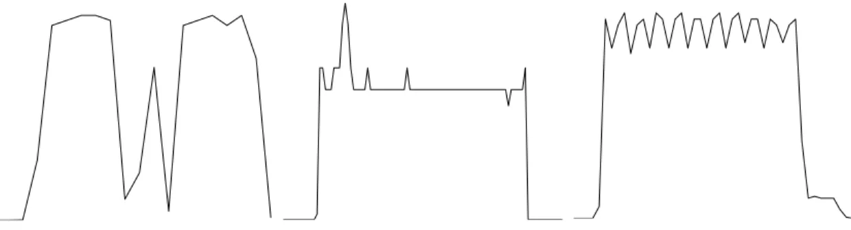
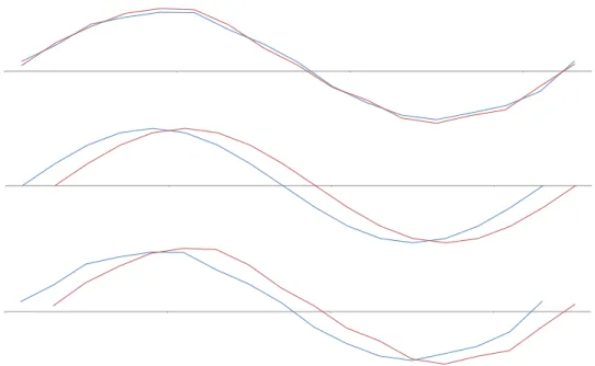
Local similarity of shape can inform prediction and other tasks, but can also enhance understanding of time-series data. Consider Figure 1.1. Examined as a whole, there are long stretches of the series where they barely differ. In the middle third, however, are local shapes that differ substantially from series to series. By examining local-shape-based similarity, we can ensure that these differences are not swamped by the general similarities, but are used to distinguish the series, exactly as they are under intuitive visual inspection.
Local shapes are uniquely comprehensible aspects of time series. A very long time series cannot be grasped intuitively, which makes systems based on global sim-ilarity of shape uninformative. Data-mining techniques based on auto-correlation or Fourier transformation can reduce comprehensibility, and make visual interpretation very difficult, especially for non-specialists. Our hypothesis is that local similarity of shape offers an intuitively comprehensible way of understanding long time series. In addition to this, we believe that local similarity of shape can be used to improve the
quantitative aspects of time-series data mining.
Figure 1.1: Four ECG time series from the ECGFiveDays dataset. The beginning third and final third of the series are very similar, differing only a little and seemingly at random. The middle third, in contrast, has a number of local shapes that differ substantially between the series.
We apply the subsequence-based approach to supervised data mining, showing that time-series classification accuracy can be improved by transforming the data into a space of local shapes, and that rule induction for partial classification of time series can be fruitfully applied to the transformed data. We also investigate unsupervised data mining, finding approximately repeated subsequences in time-series data that can provide primitives for future data mining, and can aid in understanding and analysing the data.
clustering, rule induction, and repeated pattern mining over the course of this thesis; these contributions are detailed in Section 1.2.
1.1
Research objectives
The overall objective of this thesis is to address the following question: how best can we use methods based on local similarity of shape for mining time-series data? More specifically, the question can be broken down into two sub-questions:
1. How can notions of local similarity of shape be used to create high-performing approaches to existing time-series data-mining tasks?
2. How can the interpretability offered by methods based on local similarity of shape be maximised without compromising performance?
1.1.1
Objectives
The objectives of the thesis, which address the research questions, are as follows:
1. Develop and test subsequence-based representations for time-series.
2. Create and refine algorithms and methods for discovering and extracting sub-sequences to represent locally-similar features.
3. Implement and test approaches to make best use of the representations for solving specific data-mining problems.
4. Design methods and representations that maximise interpretability without sub-stantially diminishing performance.
1.1.2
Challenges
Achieving the objectives listed in the previous subsection, and hence satisfactorily answering the research questions, requires surmounting three main challenges:
1. Existing methods for time-series classification, with which a large proportion of this thesis is concerned, are well developed and highly accurate. The new meth-ods proposed must offer substantial improvements above the existing methmeth-ods, either in terms of accuracy or interpretability. In terms of classification accu-racy, benchmark approaches must be bettered, or at least equalled (if there is some other advantage to using local similarity, e.g. increased interpretability). This is challenging, because the benchmark level of accuracy is high.
2. One strength of the local-shape-based approach is interpretability. Interpretabil-ity is inversely proportional to complexInterpretabil-ity; to maximise interpretabilInterpretabil-ity,
com-plexity must be minimised. Over simplification, however, is detrimental to
performance. A key challenge in answering the overriding research question of this thesis is balancing interpretability with performance.
3. Discovering and extracting representative subsequences is a complex problem; the time complexity of proposed algorithms must be reasonable enough that they can be tested on a range of problems. The same is true of dimensionality-reduction methods to improve interpretability: the time complexity of the method must not be so high as to exclude reasonable applications. This is partly so that the new methods can be deployed in a wide range of situations, and partly to ensure that they can be tested on a large number of datasets to ensure robust results.
In overcoming these challenges and answering the overriding research question, we have made a number of novel contributions, listed in the next section.
1.2
Novel contributions
1.2.1
Shapelet transform and ensemble classifier
In Chapter 5, we propose and extensively test a shapelet transform, using heteroge-neous ensemble classification, that provides significantly better classification accuracy than the benchmark approach to time-series classification (1NN with DTW distance and cross-validated warping window size). It is also significantly more accurate than the leading shapelet-based approaches (Fast Shapelets and Logical Shapelets).
Work on the shapelet transform is published in [88]; legacy results are published in [119]. Many of the results of our extensive experimentation with the up-to-date version of the transform and the heterogeneous ensemble classifier are used in [9] (currently under review), which combines a large number of different transforms, distance measures, and classifiers to create a more accurate time-series classification system than anything in the current literature. The shapelet transform with ensemble classifier is one of the best-performing elements of the COTE ensemble [9].
1.2.2
Clustering shapelets and binary transformation
In Chapter 5, we propose and test a novel, parameterless approach to clustering shapelets. Our method finds the correct number of shapelets for a given problem using Minimum Description Length, maintaining classification accuracy while reducing the number of shapelets to increase interpretability. This is a useful feature for reducing the dimensionality of our shapelet-transformed datasets, but more importantly, shows that clustering with MDL could be suitable in the more general case for correctly clustering time-series subsequences.
Following on from our clustering method in Chapter 5, we propose a binary trans-form for shapelet data that we believe offers the most interpretable trans-form of shapelet-transformation. The binary-transformed data sacrifices a small amount of accuracy for some (but not all) datasets, but delivers high interpretability, with each series of the transformed data represented by binary values indicating the presence or absence of each shapelet in that series. Models built on this data have the potential to be comprehensible to end-users working in domains like medicine and finance, where every decision must be justifiable.
1.2.3
Partial classification of binary-shapelet data
In Chapter 6, we propose a partial classification method based on association rules that significantly improves upon the accuracy of our state-of-the-art classifier in cases where the ensemble predicts poorly. It also offers highly interpretable insight into the relationship between the data and the class in the form of association rules that hold over binary shapelets.
Our approach is best used in one of two ways: as a supplement to the ensem-ble classifier to improve performance for poorly-predicted classes of interest, or as a general-use, highly interpretable approach to analysing the relationships between the attributes of the data and the class label.
1.2.4
BruteSuppression
In Chapter 6, we propose BruteSuppression, a novel algorithm for reducing rule set
size that can dramatically decrease the number of rules in the rule set with no loss of classification accuracy. This creates more compact and interpretable rule sets. The BruteSuppression algorithm is published in [86], along with a large amount of analysis into its effects on the distribution of rules in rule sets. Here, we restrict our qualitative analysis to a single standard dataset (Adult [164]), and focus on the
quantitative effects of BruteSuppression on the size and predictive performance of rule sets built on binary-shapelet data.
1.2.5
Interestingness measures for partial classification rules
In Chapter 2, we show that twelve commonly used interestingness measures impose the same ordering on a partial classification rule set as confidence, making them redundant as assessment tools for these rule sets. Many algorithms, including Apriori, allow the user to select a measure other than confidence to use for rule induction, and we require an interestingness measure for the BruteSuppression algorithm proposed in Chapter 6. By proving that there is no tangible difference between these measures in terms of partial classification, we justify our use of confidence as an interestingness measure, and also clarify the choice of interestingness measure for partial classification in the general case.
This work is published in [87].
1.2.6
Mining approximately repeated patterns
In Chapter 7, we propose three novel algorithms for finding approximately repeating patterns in time series, testing them extensively on bespoke synthetic data, and on a real-world electrical device disambiguation problem. We show that a subsequence-based approach can be used to detect specific instances of distinct device usage, suggesting that motifs could be suitable for similar problems in other domains where approximately repeated patterns must be discovered in time series.
1.3
Thesis structure
The thesis is structured as follows:
• In Chapter 3, we give an up-to-date overview of the shapelet approach and motifs.
• Chapter 4 describes the datasets we have used for our experiments; we cover
existing time-series problems and our own contributed data.
• In Chapter 5, we propose and test a shapelet transform with an ensemble
clas-sifier that outperforms the benchmark time-series classification method and the best published shapelet-based classifiers. We also create a novel parameter-less clustering method for finding the ‘right’ number of shapelets for a given problem, and a binary transform for shapelets that maximises interpretability.
• Chapter 6 describes a system for partial classification using binary-shapelet data that can significantly improve upon the performance of the ensemble classifier in certain cases, and which offers a highly interpretable model. We also propose a novel algorithm that substantially reduces the size of association rule sets without compromising partial classification or removing potentially interesting rules.
• In Chapter 7, we propose three novel algorithms for finding approximately
re-peating patterns in time series, testing them extensively on bespoke synthetic data, and on a real-world electrical device disambiguation problem.
• Chapter 8 presents our conclusions and suggests directions in which our work
Time-series Classification and Rule
Induction
Section 2.10 of this chapter is based on a novel analysis of existing interestingness measures published in the following paper:
J. Hills, L. Davis, A. Bagnall
Interestingness Measures for Fixed Consequent Rules
Proceedings of the 13th International Conference on Intelligent Data Engineering and Automated Learning, Lecture Notes in Computer Science, pages 68–75, Springer-Verlag: 2012.
2.1
Introduction
We focus our interest on three time-series data-mining tasks: time-series classification, partial classification of time series with association rules, and the discovery of repeated patterns in time series. We address the background of the final task in Chapter 3, as our work is very dependent on the particular representation we use for the repeated patterns, and the information is better presented in context. In the first half of this chapter, we address time-series classification; the subject of the second half is induction of partial classification rules.
In Section 2.2, we discuss time-series classification; we make novel contributions to this area in Chapters 5 and 6. We discuss the classifiers we have used in Section 2.3, and dynamic time warping, a benchmark approach in time-series classification, with which we compare our method, in Section 2.4. We use an ensemble classifier; the relevant background is given in Section 2.5. In Section 2.6, we discuss the two main tests we use to compare classifiers: the Wilcoxon Signed Rank Test (Section 2.6.1) and the Friedman Test with post-hoc Nemenyi test (Section 2.6.2). We also describe the visual method we use to display our results: the critical-difference diagram (Sec-tion 2.6.3).
In Section 2.7, we shift focus from classification to partial classification with as-sociation rules, a field to which we make a novel contribution in Chapter 6. We describe the association rule algorithm we use, Apriori, in Section 2.8. In Section 2.9, we discuss interestingness measures. Which interestingness measures to use in Chap-ter 6 is an important design choice, motivated by the theoretical assessment given in Section 2.10.
2.2
Time-Series classification (TSC)
2.2.1
Classification
In classification, a learner uses labelled training examples to search its hypothesis space for a classifier. The classifier generalises from the training examples to predict labels for new examples. Different learners use different strategies to search their hypothesis space; the hypothesis space itself varies from learner to learner.
A size N dataset D is a set of instances {D1, D2, . . . , DN}, where each instance
Di = {< xi,1, xi,2, . . . , xi,m >, ci} consists of a set of m attribute values and a class
label. The order of the attributes is unimportant, and interaction between variables is considered to be independent of their relative positions. D is split into a training
setDtrain and a test setDtest, such thatDtrain ∪Dtest =D and Dtrain∩Dtest=∅.
A classifier is trained by inputting Dtrain to the learner. The algorithm uses
the labelled examples to infer the relationship between the attributes and the class label. Given an instance, the trained classifier produces a prediction based on the attributes of the instance. The accuracy of the classifier’s predictions on unseen data
(often the instances in Dtest) is calculated to provide an estimate of how well the
classifier represents the relationship between the attributes and the class label. We focus on a sub-problem within classification: time-series classification (TSC).
2.2.2
Time-series
A time series is a sequence of data that is typically recorded in temporal order at fixed intervals. Suppose we have a set of N time series T= {T1, T2, . . . , TN}, where
each time series Ti has m real-valued ordered readings Ti =< ti,1, ti,2, ..., ti,m >, and
a class label ci. We assume that all series in T are of length m, but this is not a
requirement (see [91] for discussion of this issue). Given a dataset T, the time-series
1 512
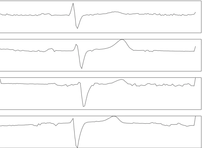
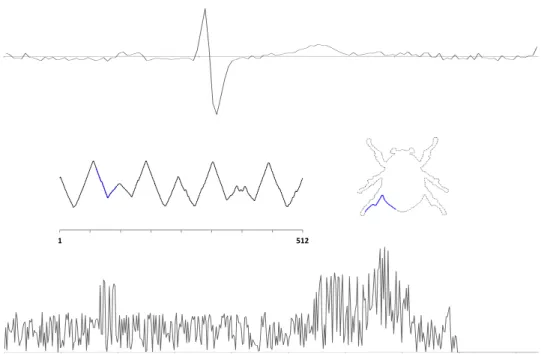
Figure 2.1: Top: a time series representing electrical activity in the heart. Middle: a 1-D series (left) representing the outline of an image (right). Bottom: an ordered series representing a spectrograph of a sample of beef.
series to the space of possible class labels.
In TSC, a class label is applied to an unlabelled set of data. The attributes of time-series objects represent ordered data, typically the same quality measured over time. Data need not be ordered temporally to be treated as a time series, however. Examples of sequence data include temporally-ordered data, such as recordings of electrical activity in the heart (Figure 2.1 top), spatially-ordered data, e.g. images (Figure 2.1 middle), and other ordered data, for example spectrographs (Figure 2.1 bottom). For time-series data, the order of the variables is often crucial for finding the best discriminating features.
TSC problems occur in a variety of domains, including image processing [143], robotics [166], healthcare [146], and gesture recognition [122].
Various algorithms are used for TSC, including tree-based classifiers (e.g. C4.5), lazy classifiers (e.g. k-nearest neighbour (kNN)), and probabilistic classifiers (e.g.
Naive Bayes). TSC research has focused on alternative distance measures for kNN classifiers, based on either the raw data, or on compressed or smoothed data (see [51] for a comprehensive summary). This idea has propagated through current research. For example, Batistaet al. state that“there is a plethora of classification algorithms that can be applied to time series; however, all of the current empirical evidence sug-gests that simple nearest neighbor classification is very difficult to beat”[12]. Recently, several alternative approaches have been proposed, such as weighted dynamic time warping [99], support vector machines built on variable intervals [150], tree-based en-sembles constructed on summary statistics [46], and a fusion of alternative distance measures [29].
There are three general types of within-class similarity that may be relevant to TSC: similarity in time, similarity in change, and similarity in shape.
Similarity in time encompasses time series that are observations of variation of a
common curve in the time dimension. kNN classifiers with elastic distance measures
perform well when classes are distinguished by this kind of similarity [51, 7]. Similarity in change occurs when series of the same class have a similar form of autocorrelation. A common approach used for TSC with this kind of similarity is to fit an Auto-regressive Moving Average (ARMA) model and base classification on differences in the model parameters [8]. Our interest is focused on similarity in shape.
2.2.3
Similarity in shape
Similarity in shape is a feature of time series that are distinguished by some
phase-independent sub-shape that may appear at any point in the series. Aglobal sub-shape
is one that approaches the length of the series. A local sub-shape is one that is short relative to the length of the series, and may appear anywhere in the series.
Figure 2.2: Globally similar sine waves. Top: noise in measurement. Middle: noise
in indexing. Bottom: noise in measurement and indexing.
the same class, transformation into the frequency domain is likely to be fruitful [173, 98, 30, 7].
If a global common sub-shape is found within instances of the same class and there is little phase shift, kNN classifiers with elastic distance measures will perform well [51, 7]. Variation around the underlying shape is caused by noise in observation, and also by noise in indexing, which may cause a slight phase shift. Consider two series produced by the same sine function. Noise in measurement alters values in the series; noise in indexing offsets the sine wave (Fig. 2.2).
A standard example of this global similarity of shape with little phase shift is the Cylinder-Bell-Funnel artificial dataset, where there is noise around the underlying shape and in the index where the shape transitions (see Figure 2.3).
Locally-similar series have common sub-shapes that are short relative to the se-ries. Local similarity can be obscured by noise in measurement; in addition, if the similar subshapes appear at very different indexes, they will be difficult to detect
0 20 40 60 80 100 120 140 Time Cylinder 0 20 40 60 80 100 120 140 Time Bell 0 20 40 60 80 100 120 140 Time Funnel
Figure 2.3: Series from the Cylinder-Bell-Funnel dataset. Each series represents a noisy, offset instance of a particular curve, specific to one of the three types. From left to right: Cylinder, Bell, Funnel.
Class 0
Class 1
Class 0
Class 1
Figure 2.4: Time series of two different classes. A global approach will pair the series incorrectly, due to the offset in the time dimension. A local approach will pair the instances correctly, as the subsequences are exact matches.
with global approaches (Fig. 2.4). Transformation into the frequency domain and
kNN with elastic distance measures might not discriminate well between the classes.
The shapelet approach is tailored to discriminate on local similarity (see Chapters 3 and 5).
2.3
Classifiers
We make use of a number of standard classifiers: C4.5, kNN,Naive Bayes, Bayesian
Network, Random Forest, Rotation Forest, and two Support Vector Machines. We choose these classifiers as they are widely used, are diverse in their operation, and are
all implemented in the WEKA machine learning tool kit [78].
Naive Bayes - referring the reader to [79]. The more complex classifiers operate as follows. A Bayesian network is an acyclic directed graph with associated probability distributions [63]. It predicts class labels without assuming independence between variables. The Random Forest algorithm classifies examples by generating a large number of decision trees with controlled variation, and taking the modal classification decision [24]. The Rotation Forest algorithm trains a number of decision trees by applying principal components analysis on a random subset of attributes [151]. A support vector machine finds the best separating hyperplane for a set of data by selecting the margin that maximises the distance between the nearest examples of each class [38]. It can also transform the data into a higher dimension to make it linearly separable.
2.4
Dynamic time warping
Dynamic Time Warping (DTW) distance is used withkNN classifiers in TSC to miti-gate problems caused by distortion in the time axis [18, 144]. Measuring the DTW dis-tance between two length m series, t =< t1, t2, . . . , tm >, and s =< s1, s2, . . . , sm >,
involves computing the m×m distance matrix M, where Mi,j = (ti−sj)2.
A warping path, P, is a set of points that defines a traversal of M, where e and
f are row and column indices respectively:
P =<(e1, f1), . . . ,(em, fm)> .
The Euclidean distance, for example, is the path that follows the diagonal of M,
P =<(e1, f1),(e2, f2), . . . ,(em−1, fm−1),(em, fm)>. All warping paths must begin at
point (1,1) and end at point (m, m), and satisfy the conditions (ei+1−ei) ∈ {0,1}
and (fi+1−fi)∈ {0,1}.
Other constraints can be placed on the warping paths. One common additional
the maximum allowable distance between any pair of indexes in the warping path. This reduces computation time, and may prevent some pathological warping paths, for example paths that map many points in one series to the same point in the other. Setting the warping window through cross validation significantly improves the accuracy of 1NN with DTW distance [144, 117].
The DTW distance between two series is defined as the total distance covered by the shortest warping path. The optimal path is found using dynamic program-ming [144]. Extensions to DTW have been proposed in [101, 99, 74].
Extensive experimentation has led to 1NN with DTW distance (and cross valida-tion to select the size of the warping window) being regarded as the benchmark for TSC [51, 117]. The evidence [51, 152, 174] suggests that, for smaller datasets, elastic similarity measures such as DTW outperform simple Euclidean distance. However,
as the number of series increases, “the accuracy of elastic measures converges with
that of Euclidean distance” [51].
2.5
Ensemble classifiers
An ensemble of classifiers combines a set of base classifiers by fusing the individual predictions to classify new examples [50, 127]. Majority vote fusion [106] is an in-tuitive approach; for alternative fusion schemes see [104]. Beyond simple accuracy comparison, there are three common approaches to analyse ensemble performance: diversity measures [105, 162], margin theory [127, 145], and Bias-Variance decompo-sition [13, 23, 60, 97, 163, 167]. These have all been linked [162, 52].
The key concept in ensemble design is the requirement that the ensemble be diverse [50, 70, 76, 80, 123, 154]. Diversity can be achieved in the following ways:
• Employing different classification algorithms to train each base classifier to form a heterogeneous ensemble.
• Changing the training data for each base classifier through a sampling scheme or by directed weighting of instances [22, 24, 59, 170].
• Selecting different attributes to train each classifier [24, 89, 151].
• Modifying each classifier internally, either through re-weighting the training
data or through inherent randomization [57, 59].
Ensembles have been applied to time-series data-mining problems, and have shown
promising results [29, 46, 150]. For example, Denget al. propose a version of random
forest [24] that uses the mean, slope, and variance of subseries as the attribute space, offering better accuracy than random forest used on the raw data [46]. Buza [29], and Lines and Bagnall [117], use ensembles of different distance measures to improve TSC accuracy.
2.6
Comparing classifiers
Demˇsar [45] discusses tests for comparing classifiers over multiple datasets. He argues that the appropriate test for comparing two classifiers over multiple datasets is the Wilcoxon Signed Rank test; for comparing multiple classifiers over multiple datasets, he advocates the Friedman test with post-hoc Nemenyi test.
2.6.1
Comparing two classifiers: the Wilcoxon Signed Rank
test
Demˇsar [45] recommends using the Wilcoxon Signed Rank test to compare two clas-sifiers over multiple datasets for three reasons. First, the Wilcoxon Signed Rank test does not require that classfication accuracies across different problem domains be commensurable. Accuracies can be wildly different across problems; using ranks prevents ten differences of 0.01 being balanced by a single difference of 0.1. Second,
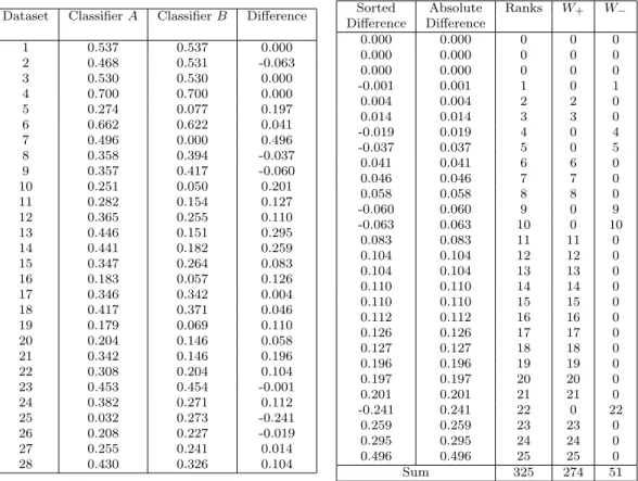
Table 2.1: Left: accuracies for two classifiers over 28 datasets with differences. Right: differences sorted by absolute value, ranks, and W+ and W− statistics.
Dataset ClassifierA ClassifierB Difference
1 0.537 0.537 0.000 2 0.468 0.531 -0.063 3 0.530 0.530 0.000 4 0.700 0.700 0.000 5 0.274 0.077 0.197 6 0.662 0.622 0.041 7 0.496 0.000 0.496 8 0.358 0.394 -0.037 9 0.357 0.417 -0.060 10 0.251 0.050 0.201 11 0.282 0.154 0.127 12 0.365 0.255 0.110 13 0.446 0.151 0.295 14 0.441 0.182 0.259 15 0.347 0.264 0.083 16 0.183 0.057 0.126 17 0.346 0.342 0.004 18 0.417 0.371 0.046 19 0.179 0.069 0.110 20 0.204 0.146 0.058 21 0.342 0.146 0.196 22 0.308 0.204 0.104 23 0.453 0.454 -0.001 24 0.382 0.271 0.112 25 0.032 0.273 -0.241 26 0.208 0.227 -0.019 27 0.255 0.241 0.014 28 0.430 0.326 0.104
Sorted Absolute Ranks W+ W− Difference Difference 0.000 0.000 0 0 0 0.000 0.000 0 0 0 0.000 0.000 0 0 0 -0.001 0.001 1 0 1 0.004 0.004 2 2 0 0.014 0.014 3 3 0 -0.019 0.019 4 0 4 -0.037 0.037 5 0 5 0.041 0.041 6 6 0 0.046 0.046 7 7 0 0.058 0.058 8 8 0 -0.060 0.060 9 0 9 -0.063 0.063 10 0 10 0.083 0.083 11 11 0 0.104 0.104 12 12 0 0.104 0.104 13 13 0 0.110 0.110 14 14 0 0.110 0.110 15 15 0 0.112 0.112 16 16 0 0.126 0.126 17 17 0 0.127 0.127 18 18 0 0.196 0.196 19 19 0 0.197 0.197 20 20 0 0.201 0.201 21 21 0 -0.241 0.241 22 0 22 0.259 0.259 23 23 0 0.295 0.295 24 24 0 0.496 0.496 25 25 0 Sum 325 274 51
the Wilcoxon Signed Rank test does not assume normality for the distribution of the accuracies; this is appropriate, as we cannot rely on this assumption. Third, because it uses ranks, the Wilcoxon Signed Rank test is not badly affected by outliers. For these reasons, we perform all pairwise comparisons of classifiers over multiple datasets using the Wilcoxon Signed Rank test.
The Wilcoxon Signed Rank test [172] is a non-parametric test. We use it to compare the accuracies of two classifiers over a number of different datasets (for example, Table 2.1). The difference is computed for each pair of accuracies. The list of differences is sorted by absolute value. The non-zero absolute differences are ranked in ascending order of absolute value (Table 2.1). The test statistics are created by summing the ranks for positive differences (W+) and negative differences (W−).
We take Nr to be the highest rank (in Table 2.1, 25). If Nr ≥15, the distribution
of W+ orW− (we concentrate onW+, but W− can be substitutedmutatis mutandis)
approaches the normal distribution where:
µW+ = Nr(Nr+ 1) 4 , (2.6.1) σW+ = r Nr(Nr+ 1)(2Nr+ 1) 24 . (2.6.2)
Hence, the statistic:
Z = W+−µW+ σW+
(2.6.3) can be used to test for significant difference where Nr≥15 (for cases where Nr <15,
a statistical table can be used to find critical values, see for example [168]).
In our example (Table 2.1), Nr = 25, W+ = 274, µW+ = 162.5, and σW+ =
37.165. Hence,Z = 27437−.165162.5 = 3; there is a statistically significant difference between Classifier A and Classifier B at a significance level of 0.01.
Where we compare two classifiers over multiple datasets, we use the Wilcoxon Signed Rank test with a significance level of 0.01.
2.6.2
Comparing multiple classifiers: the Friedman Test with
post-hoc Nemenyi test
Demˇsar [45] argues that a Friedman test [61, 62] with post-hoc Nemenyi test [133] is the best way to compare multiple classifiers over multiple datasets. The Friedman test does not rely on the same assumptions as the repeated measures ANOVA, which include the assumption that the samples (i.e. the accuracies) are drawn from a normal distribution, and the assumption of sphericity, which requires that the variances of the differences between all possible pairs of groups are equal. When comparing classifiers, there is no guarantee that these assumptions will not be violated. Hence, we prefer the Friedman test to the Anova for multiple comparisons.
The Friedman test ranks each classifier separately on its performance on each dataset, assigning ranks in ascending order (rank 1 for the best classifier, average ranks where classifiers tie). rij is the rank of the jth of k classifiers on the ith of N
datasets, and Rj = N1 Pirji, the average ranks of the algorithms. The Friedman
statistic: χ2F = 12N k(k+ 1) " X j R2j − k(k+ 1) 4 # (2.6.4) is used to compute: FF = (N −1)χ2F N(k−1)−χ2 F , (2.6.5)
which follows an F-distribution withk−1 and (k−1)(N−1) degrees of freedom. We use theFF statistic to determine whether there is a significant difference between the
classifiers, testing the null hypothesis (that there is no difference) at a significance level of 0.01.
If the Friedman test allows us to reject the null hypothesis (i.e. there is a significant difference between the classifiers), we perform a post-hoc Nemenyi test. In a Nemenyi test, the performance of two classifiers is significantly different if the average ranks of the two classifiers differ by at least the critical difference:
CD =qα
r
k(k+ 1)
6N (2.6.6)
The critical valuesqαare based on the Studentized range statistic divided by
√
2 (see, for example, [168], for statistical tables). If the difference in average rank between two classifiers (where we have rejected the null hypothesis using the Friedman test) exceeds the critical difference, we take the classifiers to be significantly different.
Where we compare multiple classifiers over multiple datasets, we use the Friedman test with post-hoc Nemenyi test at a significance level of 0.01.
2.6.3
Critical-difference diagram
When comparing multiple classifiers over multiple datasets, we present our results perspicuously using a critical-difference diagram [45]. An example critical-difference diagram is shown in Figure 2.5.
CD 5 4 3 2 1 2.24 A 2.61 B 2.77 C 3.52 D 3.86 E
Figure 2.5: Example critical-difference diagram comparing five classifiers over multi-ple datasets. A pair of classifiers is significantly different if they do not belong to the same clique, represented by the black bars.
In Figure 2.5, each classifier is aligned along the axis based on its average rank over
the datasets. The black bars show the cliques. If two classifiers belong to the same
clique, there is no significant difference between their performances on the datasets.
In Figure 2.5, classifiers A, B, and C all belong to the same clique, meaning there
is no significant difference between their performances on the datasets. There is a significant difference between classifier E and classifiers A,B, andC, as they do not belong to the same clique.
Where we compare multiple classifiers over multiple datasets, we will present the results using critical-difference diagrams.
2.7
Mining association rules
The previous sections have focused on classification. The second half of this chapter is focused on partial classification (nugget discovery) through association rules, which is the method we employ to make the novel contribution in Chapter 6. The goal of partial classification is to discover association rules that reveal characteristics of some pre-defined class(es); such rules need not cover all classes or all records in the dataset [4, 44, 43]. Rule induction algorithms (e.g. [2]) can be used to generate a set of partial classification rules. Partial classification rules provide a comprehensible set of predictors for certain outcomes. We are interested in partial classification rules with a single, fixed consequent, i.e. rules for a single class. As well as as their use for partial classification, association rules can provide insight into the data [2]. Association rules allow the end-user to achieve an understanding of the data that may not be forthcoming from other models (e.g. neural network approaches, which provide predictive power without an immediately comprehensible model, see [14]).
The problem of discovering association rules from large datasets is formulated in [2] as the market basket problem: given a large set of transactions, how can we efficiently discover the associations that hold between various items? Their approach was not targeted at discovering associations with a particular class label; rather, all associations were discovered.
The general problem of association rule mining for partial classification is as fol-lows. Given a labelled dataset and one class label from that dataset (designated the target), find all associations (subject to certain constraints) that hold between other attributes and the target class label.
Association rules take the form:
where the antecedent and consequent of the rule are some conjunction of Attribute Tests (ATs). An AT (see, e.g. [149]) takes the form: < AT T, OP, V AL >, where
ATT is one of the attributes of the records in the dataset, OP is one member of the
set {<,≤, >,≥,=} and VAL is a permissible value for the attribute. In Chapter 6, we use Apriori on binary data. Hence, each AT is of the form: < AT T,=,{0,1}>;
an example AT is {Shapelet1} = {0}. An example rule is: {Shapelet1} = {0} ⇒
{Class}= 1. The class attribute is the only non-binary attribute in the data we use for rule induction in Chapter 6.
We use N(A) to indicate the number of records in the dataset that satisfy the
antecedent of a given rule, and N(C) for the number of records that satisfy the
consequent of the rule. N(U) is used to represent the size of the dataset. The
propositional connectives ∧, ∨, and ¬ are used to indicate conjunction, disjunction,
and negation. For example, N(A∨ ¬C) represents the number of records that satisfy
the antecedent or the negation of the consequent.
For any association rule R = A ⇒ C (where A and C are conjunctions of ATs
representing the antecedent and consequent of the rule respectively), the support of the rule (Sup(R)) is calculated as follows:
Sup(R) =N(A∧C) (2.7.1)
which is the number of records in the dataset that satisfy both the antecedent and
the consequent of the rule. The confidence of R (denoted Conf(R)) is:
Conf(R) = N(A∧C)
N(A) . (2.7.2)
The confidence of a rule is the support of the rule divided by the support of the antecedent. The coverage [124] ofR (Cov(R)) is calculated as:
Cov(R) = N(A∧C)
The coverage of a rule is the support for the rule divided by the support for the consequent, and represents the proportion of records satisfying the consequent that are correctly covered by the rule.
For any dataset that is not trivially small, there will be a large number of potential rules, and it is necessary to have an efficient algorithm to mine the data. There are many different algorithms for mining association rules, for example [3, 14, 112, 36, 149]. We use the Apriori algorithm [3] in Chapter 6; the algorithm is described in the next section.
2.8
Apriori
We use the Apriori [3] association rule discovery algorithm to generate rule sets for
our experiments (see Algorithm 1). The Apriori algorithm operates on itemsets. An
itemset is a combination of items, where each item is an AT. Itemsets are arbitrarily ordered (this ordering is used in the generateCandidates procedure). We denote the
kth AT as Ik. The algorithm first determines which itemsets are large (above the
minimum support constraint) and their support (it is common to use a proportion or
percentage for the minimum support parameter; in Algorithm 1, minsup is assumed
to be a count, so proportions, for example, need to be multiplied by the number of records). To determine the large itemsets, Apriori establishes which pairs of items have support above the minimum; these items are retained for the next pass, which finds the sets of three items that have support above the minimum, and so on, un-til no itemsets have sufficient support (or the maximum number of items has been reached). The maximum support of any itemset containing n items {I1, I2, ..., In}
is M in(Sup(I1), Sup(I2), ..., Sup(In)), so this approach is computationally more
ef-ficient than assessing every possible itemset. Itemsets are pruned if they have any subset that has not appeared in a previous pass, further reducing the final set of large
itemsets, denoted LT ot.
The generateCandidatesprocedure produces candidate itemsets (Ck) ofk items
from the set Lk−1 (Algorithm 2). In the join stage, any k −1 itemsets that differ
only in their k−1th item are combined to form a k itemset including the k −1th
item of both itemsets. In the prune stage, any itemset generated in the join stage
that includes ak−1 itemset not included in the setLk−1 is removed from the setCk.
The set is returned, the support is calculated, and the set of large k-itemsets, Lk is
formed from those candidate itemsets exceeding the minimum support [3].
Algorithm 1 apriori(D, the set of all instances, minsup, the minimum support
parameter, minconf, the minimum confidence parameter)
L1 ← {large 1-itemsets}// Generate all large 1-itemsets
k←2
while Lk−1 6=∅ do
Ck← generateCandidates(k, Lk−1) // New candidate itemsets
for all candidate itemsets c∈Ck do
c.count←0
for all instances t∈D do
Ct ←Ck∩ P(t) // Candidate itemsets that are subsets of t
for all candidate itemsets c∈Ct do
c.count+ + Lk ← {c∈Ck:c.count≥minsup} k+ + LT ot← S kLk
RS =∅; // Generate rule set
for all large k itemsetslk∈LT ot wherek ≥2 do
H ← {consequents of rules derived from lk with one item in the consequent}
RS ←RS ∪generateRules(k, lk,1, H)
return RS
Once the setLT otis established, rules are generated by the proceduregenerateRules
(Algorithm 3). For each large itemset (lk), every subsetaproduces a rulea⇒l−{a},
which is added to the rule set (RGR) if the confidence of the rule exceeds theminconf
parameter. The algorithm shown here will generate all association rules above the minimum support and confidence thresholds. To generate association rules with a
Algorithm 2generateCandidates(k, Lk−1, the set of all largek−1-itemsets) Ck ← ∅ for allX ∈Lk−1, Y ∈Lk−1 do if (X− {Xk−1}=Y − {Yk−1})∧(Xk−1 6=Yk−1) then c←X∪Y Ck ←Ck∪ {c} for allc∈Ck do
for all k−1 subsets ofc, sdo if s /∈Lk−1 then
Ck←Ck− {c}
return Ck
fixed, single AT consequent, we generate only itemsets that contain the consequent,
and replace the generateRules procedure with an assessment of the confidence of
the rule R = I− {c} ⇒c, where I is the itemset and c is the item representing the
fixed consequent.
Algorithm 3generateRules(k, lk, ak-itemset, m, H, a set of consequents)
RGR← ∅
if k > m then
m+ +
for all h∈H do
conf ←support(lk)/support(lk−h)
if conf ≥minconf then
r ←< rule, conf,support(lk)>, where rule= (lk− {h})⇒h
RGR←RGR∪ {r} else H ← H− {h} H ← generateCandidates(H) RGR←RGR ∪generateRules(k, lk, m, H) return RGR
The minimum support and minimum confidence parameters are used to reduce the size of the rule set, eliminating rules on the basis of counts from the dataset.
2.9
Interestingness measures
Rule set quality is assessed in terms of the quality of the individual rules in the set. The term typically used in the literature for the quality of a rule isinterestingness, and we shall adopt this convention. The rules generated by algorithms may be interesting or not. Objective interestingness measures are used to assess how interesting an association rule might be from the structure of the dataset. Support and confidence are two common measures by which the interestingness of a rule is assessed, and form the basis of most objective interestingness measures.
Blanchard et al. [20], following [138], define a rule interestingness measure as a
function from a rule onto the real numbers, which increases with N(A∧C) and
de-creases with N(A) when all other parameters are fixed. Piatetsky-Shapiro and
Fraw-ley [138] suggest that a good measure should decrease withN(C). This is restrictive, however; interestingness measures should not have any determined behaviour with regard to N(C) and N(U) [20].
In [20], rules are represented as ordered quadruples of the form:
R=< N(A∧C), N(A), N(C), N(U)> . (2.9.1)
For an association rule with a fixed consequent,N(C) andN(U) are constants. Hence, only theN(A) and N(A∧C) values of rules in a rule set vary. This greatly restricts the usefulness of this kind of interestingness measure. For example, [20], demonstrate that the orderings imposed by the confidence and lift measures on a rule set are not the same. However, the example in their proof uses different values forN(C) between rules. With a fixed consequent, it can be proved that lift and confidence impose the same ordering [15]. Thus, for association rules with a fixed consequent, the scope for objective interestingness measures to differentiate rules is greatly diminished.
confidence, and coverage (see Section 2.7), novelty [109], relative risk [4], chi-square
[72, 129], gain [65], k-measure [136], entropy [35, 129], Laplace accuracy [35],
in-terest/lift [95, 26], conviction [26, 14], and Gini [129]. Comprehensive surveys of interestingness measures can be found in [161, 33, 135].
The majority of interestingness measures are based on counts, such that differ-ent rules that happen to have the same counts have the same value. Over 100 of these measures are documented; however, in [15], the authors demonstrate that many different measures impose the same partial ordering on a rule set. In Section 2.10, we apply a similar line of argument to the type of rule we are interested in: partial classification rules with fixed consequent.
Subjective interestingness is a measure of how interesting the discovered rule is to a domain expert. Researchers have tested the assumption that objective and subjective interestingness are correlated [136, 33, 111, 135]. The experiments involve ranking rules based on various objective measures and on interestingness to domain experts. The performance of certain objective measures, such as relative risk [4], uncovered negative [66], and accuracy [109], was reasonable on the medical datasets studied in [135]. The effectiveness of any individual interestingness measure for a given rule set is highly correlated to the dataset in question, suggesting that this approach is unlikely to yield any projectible insight; we do not believe that the measures that performed best in the study would perform best given rule sets created from different data.
As an approach, data mining is most useful when finding rules that are difficult to find by manual analysis, and this suggests an alternative method to discover poten-tially interesting rules. We may assume that general statistical analysis reveals good single predictors of the class of interest. Instances where the combination of predic-tors produces a surprising result (poor predicpredic-tors combining to form a good rule, or
predicted classes changing with the addition of predictors to a rule, see [32, 139]) are of particular interest because they are unlikely to be revealed by such analysis. This is particularly evident in cases where the number of predictors is high and the dataset is very large. In Chapter 6, we propose two novel interestingness measures that as-sess this quality of a rule, and use them as a supplement to count-based measures for assessing rule quality.
2.10
Selecting an appropriate interestingness
mea-sure
We wish to select a count-based interestingness measure to use in our assessment of partial classification rules. In this section, we examine a number of commonly used interestingness measures, and show that, under conditions that hold for our particular area of interest, they all impose the same ordering as confidence. This is a novel analysis of existing interestingness measures that shows they are not fit for our purpose.
We focus on partial classification rules with a fixed consequent, derived from a fixed dataset. Hence, we make the following assumptions:
1. The dataset is fixed. That is, N(U) is a constant. We do not compare rules
across datasets.
2. The consequent of the rule is fixed. That is, N(C) is a constant, as is N(¬C).
Under these assumptions, we prove theoretically that twelve interestingness mea-sures proposed in the literature are monotonic with respect to confidence. Several of the proofs rely on the following equivalence:
N(A∧ ¬C)
N(A) = 1−
N(A∧C)
Satisfaction
The formula for Satisfaction [109] is:
N(¬C)×N(A)−N(A∧ ¬C)×N(U)
N(C)×N(A) . (2.10.2)
The formula can be rearranged to give:
N(¬C) N(C) − N(A∧ ¬C) N(A) × N(U) N(C) (2.10.3)
(cancelling N(A) in the first term). The first and third terms are constants, and the second term is equal to 1−Conf idence, so satisfaction is proportional to Confidence.
Ohsaki’s Conviction
Ohsaki’s Conviction [136] is calculated as:
N(A)×N(¬C)2
N(A∧ ¬C)×N(U)2. (2.10.4)
The formula can be rearranged as:
N(A)
N(A∧ ¬C) ×
N(¬C)2
N(U)2 . (2.10.5)
By dividing both the numerator and denominator of the first term byN(A), we have:
1/N(A∧ ¬C) N(A)
which is equal to 1/(1−Conf idence); the second term is a constant. Hence, Ohsaki’s conviction is proportional to Confidence.
Added Value
The formula for the Added Value measure [179] is:
N(A∧C)
N(A) −
N(C)
N(U). (2.10.6)
Brin’s Interest/Lift/Strength
Brin’s Interest/Lift/Strength [26, 14, 48] is calculated as:
N(A∧C)
N(A) ×
N(U)
N(C). (2.10.7)
The second term is fixed, so this measure is proportional to Confidence.
Brin’s Conviction
Brin’s Conviction [26] is:
N(A)×N(¬C)
N(U)×N(A∧ ¬C). (2.10.8)
As shown in [15], the formula can be rearranged by dividing both the numerator and the denominator by N(A), giving
N(¬C)
N(U)×N(A∧ ¬C)/N(A). (2.10.9)
N(A∧¬C)
N(A) is equal to 1−Conf idence. N(U) andN(¬C) are fixed, so Brin’s Conviction is monotonic with respect to Confidence.
Certainty Factor/Loevinger
The formula for Certainty Factor/Loevinger [161, 110] is:
N(A∧C) N(A) × N(U) N(¬C) − N(C) N(¬C). (2.10.10)
Both NN((¬UC)) and NN((¬CC)) are constants, so Certainty Factor/Loevinger is proportional to Confidence.
Mutual Information
The Mutual Information measure [161] is:
log2 N(A∧C) N(A) × N(U) N(C) . (2.10.11)
The log2 function is monotonic, and NN((UC)) is a constant, so mutual information is proportional to Confidence.
Interestingness
Interestingness [178] is calculated as follows:
N(A∧C) N(A) ×log2 N(A∧C) N(A) × N(U) N(C) . (2.10.12)
Interestingness is Confidence multiplied by the Mutual Information measure. Hence, it is monotonic with respect to Confidence.
Sebag-Schonauer
The Sebag-Schonauer measure [155] is:
N(A∧C)
N(A∧ ¬C). (2.10.13)
By dividing both the numerator and the denominator by N(A), we see that the
for-mula is equivalent to Conf idence/(1−Conf idence), which is proportional to
Con-fidence. This measure is proportional to Confidence even if we relax the assumption that the consequent is fixed.
Ganascia Index
The Ganascia index [67] for a rule is:
N(A∧C)−N(A∧ ¬C)
N(A) . (2.10.14)
N(A∧ ¬C) =N(A)−N(A∧C), so the numerator is equal to:
N(A∧C)−N(A) +N(A∧C) = 2N(A∧C)−N(A). (2.10.15)
Hence, the formula can be rearranged as 2NN(A(A∧C)) − NN((AA)), which is proportional to Confidence. Like Sebag-Schonauer, Ganascia Index is proportional to Confidence even if we relax our assumption of fixed consequent.
Odd Multiplier
Odd Multiplier [69] is calculated as:
N(A∧C)×N(¬C)
N(C)×N(A∧ ¬C). (2.10.16)
We rearrange the formula as:
N(A∧C)
N(A∧ ¬C)×
N(¬C)
N(C) . (2.10.17)
The second term is a constant, and the first term is the Sebag-Shonauer measure, which is proportional to Confidence. Hence, odd multiplier is proportional to Confi-dence.
Example/counter-example Rate
We calculate the Example/counter-example Rate [94] as:
N(A∧C)−N(A∧ ¬C)
N(A∧C) . (2.10.18)
The formula can be rearranged as:
N(A∧C)
N(A∧C) −
N(A∧ ¬C)
N(A∧C) . (2.10.19)
By dividing both the numerator and the denominator of the second term byN(A), and
cancelling N(A∧C) in the first term, we have 1−1−Conf idenceConf idence, which is proportional to Confidence. This measure is proportional to Confidence without the assumption that the consequent is fixed.
2.10.1
Analysis
We have shown that a large number of commonly-used interestingness measures im-pose the same ordering on a set of partial classification rules with a fixed consequent as confidence. On the basis of this, we proceed with the view that confidence is an
appropriate interestingness measure for rule induction tasks of the type we are inter-ested in, and that there is little benefit to be gained by employing any of the other measures we have examined in detail.
2.11
Mining rules from time-series data
Mining association rules from time-series data using a market-basket approach re-quires transforming the time-series into a representation that is compatible with
Apriori (or other market-basket association rule algorithms). One canonical
ap-proach is [39], where repeated patterns are discovered in time series; the patterns are the input used for finding association rules. Keogh and Lin [100] criticise the approach in [39], and similar approaches, on the grounds that the discovered patterns are meaningless because no account has been taken of overlapping subsequences. We discuss this point in greater length in Chapters 3 and 5.
Our own contribution to the problem of finding repeated patterns in time-series can be found in Chapter 7. Our interest does not lie in discovering rules in long time series, however; we wish to discover partial classification rules that can be used for (partial) TSC. We do this by transforming the data (Chapter 5) before building rule sets (Chapter 6). Our rule induction from time series is much more closely aligned with the type of rule discovery discussed in this chapter, and with TSC, than is the approach in, for example, [39].
2.12
Conclusions
In this chapter, we describe two areas of data mining that are key to our novel contributions: TSC and partial classification using association rules.
In the first half of the chapter, we discuss classification, time-series, TSC, and our particular interest in classifying time-series by similarity in shape. Specifically
to support Chapter 5, we outline the classifiers that we use and 1NN with DTW distance (a benchmark to which we compare our method), and review ensembling, which we employ to improve accuracy. We also describe the statistical tests we use when comparing our methods with other approaches in Chapters 5 and 6.
In the second half of the chapter, we discuss partial classification with association rules, the focus of Chapter 6. We describe the algorithm we use, Apriori, and how we select interestingness measures for the algorithms and assessment methods in that chapter.
The next chapter focuses on a particular aspect of TSC that is key to our novel contributions: local similarity of shape.
Representing Time Series with
Localised Shapes
A shapelet is a time-series subsequence that can be used as a primitive for TSC based on local, phase-independent similarity in shape (Figure 3.1). Shapelet-based classification involves measuring the similarity between a shapelet and each series, then using this similarity as a discriminatory feature for classification.
In Section 3.1, we define shapelets and shapelet candidates, present a generic algorithm for shapelet discovery, and define two central concepts: shapelet distance and shapelet quality. In Section 3.2, we present and analyse a number of techniques from the literature for speeding up the shapelet search. In Section 3.3, we discuss a number of different domains where shapelets have been successfully applied to classification problems, including image outlines, motion capture, and spectrographs. In Section 3.4, we examine some extensions to the shapelet approach that have been suggested in the literature. Finally, in Section 3.5, we discuss an unsupervised use of
local-shape-based similarity, where repeated patterns, called motifs, are mined from
time-series data.
0 100 200 300 400 500 Time Series of class 0.0 0 100 200 300 400 500 Time Series of class 0.0 0 100 200 300 400 500 Time Series of class 1.0 0 100 200 300 400 500 Time Series of class 1.0
Figure 3.1: Four series from our simulated dataset (see Chapter 4). The shapelets for class 0 are highlighted in black, for class 1 in red. The simulated data demonstrates the utility of shapelets for detecting phase-independent local similarity of shape in noisy data.
3.1
Shapelet definition
A time-series dataset T = {T1, T2, ..., Tn} is a set of n time series. A length m
time series Ti =< ti,1, ti,2, ..., ti,m > is an ordered set of m real numbers. A length l
subsequence of Ti is an ordered set of l contiguous values from Ti. Ti has a set Wi,l
of (m−l) + 1 subsequences of length l. Each subsequence w=< tj, tj+1, ..., tj+l >in
Wi,l is a time series of length l where 1≤j < m−l.
A shapelet is a subsequence of one time series in a datasetT(see [180, 181]) that is
discriminative of the class of the series. A good shapelet is a subsequence found only in series of a particular class (this is for the binary case. For multi-class problems, good shapelets may appear in more than one class - the important feature is that they appear in some and not in others). Whether or not a shapelet is considered to be present in a series is determined by a distance calculation (see Section 3.1.3). Every
subsequence of every series in T is a candidate - a potential shapelet. Shapelets are
found via an exhaustive search of every candidate of length min to max. Shapelets
are normalised; since we are interested in detecting localised shape similarity, they must be invariant to scale and offset, and it is insufficient to normalise the series as a whole [140].
Ye and Keogh introduce shapelets in [180], and expand upon the research in [181]. They use a decision tree to classify with shapelets. Mueen, Keogh, and Young [130]
propose an extension from shapelets to logical shapelets. The authors also provide a
method to speed up the shapelet search by reusing information from distance
calcula-tions. McGovernet al.[125] apply the shapelet approach to weather prediction. Much
of the research into shapelets has focused on methods to speed up the shapelet search.
Chang et al. implement the shapelet search in parallel on the GPU [34]. In [73], the
authors propose a randomised search for shapelets. Heet al. experiment with
![Figure 4.1: Left: a hand x-ray from [96], annotated to show the three bones of interest.](https://thumb-us.123doks.com/thumbv2/123dok_us/9013481.2799184/85.918.191.789.331.599/figure-left-hand-x-ray-annotated-bones.webp)