New microarray image segmentation using Segmentation Based Contours method

(1)

Louisiana Tech University

Louisiana Tech Digital Commons

Doctoral Dissertations

Graduate School

Winter 2013

New microarray image segmentation using

Segmentation Based Contours method

Yuan Cheng

Follow this and additional works at:

https://digitalcommons.latech.edu/dissertations

Part of the

Applied Mathematics Commons

,

Applied Statistics Commons

,

Biomedical

(2)

NEW MICROARRAY IMAGE SEGMENTATION USING

SEGMENTATION BASED CONTOURS METHOD

by

Yuan Cheng, B.S., M.S.

A Dissertation Presented in Partial Fulfillment o f the Requirements for the Degree

Doctor o f Philosophy

C O L L E G E OF E N G IN E E R IN G A N D SCIEN CE LO U ISIA N A T E C H U N IV E R S IT Y

(3)

UMI Number: 3570075

INFORMATION TO ALL USERS

The quality of this reproduction is dependent upon the quality of the copy submitted.

In the unlikely event that the author did not send a complete manuscript and there are missing pages, these will be noted. Also, if material had to be removed,

a note will indicate the deletion.

UMI 3570075

Published by ProQuest LLC 2013. Copyright in the Dissertation held by the Author. Microform Edition © ProQuest LLC.

ProQuest LLC

789 East Eisenhower Parkway P.O. Box 1346

(4)

L O U I S I A N A T E C H U N I V E R S I T Y

T H E G R A D U A T E S C H O O L

OCTOBER 31, 2012

Date

W e hereby recom m end that the Dissertation prepared under our supervision by

Y uan C heng, B.S., M.S.____________________________________________________________

entitled N ew M icroarray Im age S egm entation U sin g S egm entation Based__________

C ontours M ethod

be accepted in partial fu lfillm en t o f the requirem ents for the D egree o f Ph.D . in C om putational A nalysis and M odeling_____________

y

Supervis^Kof Dissertation Research

Head o f Department C om pu tation al A nalysis and M od elin g

Department Recommendation concurred in:

Director o f Graduate Studies

Dean o f the College

A dvisory Committee Approved: ate School Dean o GS Form 13 (8/10)

(5)

ABSTRACT

The goal o f the research developed in this dissertation is to develop a more

accurate segmentation method for Affymetrix microarray images. The Affymetrix

microarray biotechnologies have become increasingly im portant in the biomedical

research field. Affymetrix microarray images are widely used in disease diagnostics and

disease control. They are capable o f m onitoring the expression levels o f thousands o f

genes simultaneously. Hence, scientists can get a deep understanding on genomic

regulation, interaction and expression by using such tools.

We also introduce a novel Affymetrix microarray image simulation model and

how the A ffymetrix microarray image is simulated by using this model. This simulation

model em braces all realistic biological characteristics and experimental preparation

characteristics, which could have different im pacts on the quality o f microarray image

during the real microarray experiment. The m ost important aspect is that this model could

provide the "ground true information,” which allows us to have a deep understanding on

different segm entation algorithms performance.

After the simulation, the new proposed segm entation algorithm Segmentation

Based Contours (SBC) method is presented as well as the modifications o f the Active

Contours Without the Edges (A CW E) method. By m odifying the A C W E method with

higher order finite difference scheme and fast scheme, we establish the new segmentation

(6)

IV

signal values obtained from the new proposed algorithm S egm entation Based Contours

method and the best currently known method. This gene expression signal com parison is

more meaningful in gene expression analysis, since it represents the whole gene

expression level rather than the small transcripts hybridization abundance level. Different

types o f experimental com parison results will be presented to show that the new proposed

(7)

APPROVAL FOR SCHOLARLY DISSEMINATION

The author grants to the Prescott M emorial Library o f Louisiana Tech University

the right to reproduce, by appropriate methods, upon request, any or all portions o f this

Dissertation. It is understood that “proper request” consists o f the agreem ent, on the part

o f the requesting party, that said reproduction is for his personal use and that subsequent

reproduction will not occur without written approval o f the author o f this Dissertation.

Further, any portions o f the Dissertation used in books, papers, and other works must be

appropriately referenced to this Dissertation.

Finally, the author o f this Dissertation reserves the right to publish freely, in the

literature, at any time, any or all portions o f this Dissertation.

A uthor

Date

GS Form 14

(8)

66

67 68 70

LIST OF TABLES

Pixels matrix for one spot c e l l ...

Part o f header information for DAT file...

Part o f format description for CEL fil e ...

Data sets for simulation m o d e l ...

Data input f o r m a t ...

List o f noise p a ra m e te rs ...

List o f m anufacturing p a ra m e te rs ...

List o f hybridization p a ra m e te rs ...

List o f scanning p a ra m e te r s ...

G round truth pixels in one cell...

Segmentation results from G C O S ... .

Segmentation results from S B C ...

Intensity results c o m p a r is o n ...

System and M ATLAB inform ation...

Preliminary com parison for one block simulated image

Paired t test results for d 1 = S i g n a l true — S i g n a l sBC..

Paired t test results for d 2 — S i g n a l true — S i g n a l GC0S

Two sample t test for D1 and D2 ...

Quartiles sum m ary in fo rm atio n ...

(11)

Table 5.7: Different metrics com parisons for Canine_a one block simulated image .... 71

Table 5.8: Standard error o f performance and R s q u a r e d ... 74

Table 5.9: Sample replication size t a b l e ... 79

Table 5.10: Standard error performance com parison for C a n i n e _ a ... 80

Table 5.11: Pearson correlation com parison for C a n i n e _ a ... 81

Table 5.12: Paired t test for the SBC analyzed gene signal value from C a n in e _ a ...83

T able5.13: Paired t test for the G C O S analyzed gene signal value from Canine a 85 Table 5.14: M inkowski distance com parison for Canine a ... 87

Table 5.15: Euclidean distance metric com parison for C a n in e _ a ...89

Table 5.16: Correlation distance metric com parison results for C a n i n e _ a ...90

Table 5.17: Chebychev distance metric com parison for C anine a ... 92

Table 5.18: Summary com parison o f standard error o f perform ance and co rrelatio n ...94

Table 5.19: Summary com parison o f paired t test for SBC for C anine_a ...94

Table 5.20: Summary com parison o f paired t test for G C O S for C anine a ... 95

Table 5.21: Summary com parison o f clustering distance metrics for C a n i n e _ a ...95

fable 5.22: Two sample t test for the SBC averaged analyzed gene signal v a l u e ... 96

Table 5.23: Two sample t test for the G COS averaged analyzed gene signal v a lu e ...97

Fable 5.24: Two sample t test for D l l a n d D 1 2 ... 98

Table 5.25: Quartiles com parison information for D l l a n d D 1 2 ... 99

Table 5.26: Com parison for averaged analyzed gene signal for Canine_a group 101 Table 5.27: Summary com parison for eight groups sim ulated im a g e s ...108

Table 5.28: Paired t test for the SBC average analyzed gene signal v a l u e ... 109

(12)

Table 5.30: Two sample t test for the SBC average analyzed gene signal v a l u e ...

(13)

2

. . j ..4 .. 5 ..6 . . 8 10 . 1 1 12

21

22 26 27 28 30 30 34 35

LIST OF FIGURES

Building block o f DNA from [ 1 ] ...

D N A helix structure from [ 1 ] ...

D N A transcription from [1 ]...

Central dogm a o f molecular biology from [ 6 ] ...

c D N A microarray i m a g e ...

Affymetrix microarray im a g e ...

cD N A microarray experiment from [1 3 ]...

Affymetrix microarray chip from [ 1 2 ] ...

Probe leve desing in Affymetrix microarray from [16]

A ffymetrix microarray experiment process from [17].

Probe set structure from [28]...

Background subtractions from [28]...

G C O S microarray image analysis flo w ...

DAT file structure shown in M A T L A B ...

CEL file structure shown in M A T L A B ...

CD F file structure shown in M A T L A B ...

CH P file structure shown in M A T L A B ...

G C O S p la rf o r m ...

Simulation s t e p s ...

(14)

xii

Figure 3.3: Microarray simulation p ro c e s s ... 42

Figure 3.4: Segm ented image by S B C ...44

Figure 3.5: Original microarray image for Canine_a g e n o m e ... 47

Figure 3.6: Simulated microarray Canine a image in 4 x 4 b lo c k s ... 47

Figure 4.1: Affymetrix microarrary image segm ented by S B C ... 58

Figure 5.1: Simulated 16-block image for Canine a G e n o m e ...63

Figure 5.2: Simulated one block image for C anine_a G e n o m e ...64

Figure 5.3: Boxplot for D1 and D 2... 69

Figure 5.4: Cluster Tree for Canine a one block simulated im age...73

Figure 5.5: Regression plot using SBC signal as independent v a r ia b le ... 75

Figure 5.6: Regression plot using G COS signal as independent v a r i a b l e ...76

Figure 5.7: Residual plot I using SBC signal as independent v a ria b le ...77

Figure 5.8: Residual plot II using G COS signal as independent v a r i a b l e ...77

Figure 5.9: Boxplot for the absolute value o f D l l and D 1 2 ... 99

Figure 5.10: Clustering tree plot for the average analyzed gene signal v a l u e ... 102

Figure 5.11: Regression plot for average SBC s ig n a l...104

Figure 5.12: Regression plot for average G C O S s ig n a l... 104

Figure 5.13: Residual plot from average S B C ... 105

Figure 5.14: Residual plot from average G C O S ...106

Figure 5.15: Clustering tree for Bovine a ... 112

Figure 5.16: Clustering tree for B o v in e _ b ... 113

Figure 5.17: Clustering tree for V'itis a ... 113

(15)

xiii

Figure 5.19: Clustering tree for Y east-1... 114

Figure 5.20: Clustering tree for Yeast-2...115

Figure 5.21: Clustering tree for C anin e_ a ... 115

(16)

ACKNOWLEDGEMENTS

The writer o f this dissertation, Yuan Cheng, owes great appreciation to many

people at Louisiana Tech University. M y greatest gratitude goes to my academic advisor.

Dr. Mihaela Paun. for her precious guidance, generous encouragem ent and support to

finish my research work. It is m y great honor to be her doctoral student. This dissertation

could not have been com pleted without her help and suggestions. 1 w ould also like to

thank Dr. Weizhong Dai, Dr. Raja N assar and Dr. Andrei Paun for their warmhearted

help. From their courses, I gained a deep understanding o f M athem atics, Statistics and

Computer Science, which have been applied to m y research work. Sincere

acknow ledgem ent is further extended to Dr. Bogdan Strimbu for his kind suggestions and

guidance as a m em ber o f my advisory committee.

To my friends and family, thanks for your com pany and for your great support o f

my living and learning in the United States. I w ould like to thank my father, Wenzhang

Cheng, my mother, Jie Ji and my husband, Xiang Li, for their love, understanding and

endless encouragement. Finally. I would like to express my appreciation to all my friends.

(17)

CHAPTER 1 INTRODUCTION OF DNA AND DNA MICROARRAY

In this chapter, an overview o f the D N A microarray on the molecular biology

level, aiming at providing the appropriate background for understanding the microarray

segmentation problem will be presented.

1.1 DNA

All living cells on earth store their hereditary inform ation in double-stranded

molecules o f D N A from M olecular Biology o f the Cell [1]. These double-stranded

molecules o f D N A contain four types o f m onom ers, which form the long paired chains

based on the com plem entary rule. A (adenine), T (thymine), C (cytosine), G (guanine) are

strung together, encoding the hereditary information. By interpreting this sequence

information from a D N A strand, scientists are capable o f deciphering the hereditary

information contained in cells.

In 1869. Friedrich M iescher first discovered the nucleic acid from his experiment.

In 1952. Alfred Hershey and M artha Chase first established that D N A was the molecules

carrying the hereditary information for all living cells [2], In 1953, Jam es D. Watson and

Francis Crick first elaborated and presented the D N A double-stranded m olecular model

[3]. This double helix model brought a significant impact on understanding the DNA

(18)

two sections. One part is called the deoxyribose with a phosphate group in Figure 1.1

The other part is called the base, which is either A. G. C or T.

building block of DNA

phosphate

sugar

i'

G

sugar

base

(G

phosphate

nucleotide

Figure 1.1 Building block o f DNA from [1]

Next, several nucleotides are connected together by the phosphate group, which

constructs the D NA strand. These two D N A strands are synthesized according to the

com plem entary structures o f the bases, where A binds to T, and G binds to C. A fter this

synthesis process, two D NA strands twist on each other to form the double helix shown in

Figure 1.2. d o u b l e - s t r a n d e d DNA A c T G G c A A T G II ... Til Ilf Tf M 11 m T G A c c g T T a C s u g a t - p h o s p h a t e h y d f o g e n - b o n d e d b a c k b o n e b a s e p a irs DNA d o u b l e h e h x C A 1 -A A _T C TVi G 11T C A

(19)

1.2 DNA T ranscription and Translation

In order to carry the genomic information, the D NA sequence must undergo the

process o f replication and transcription with the help o f RN A (ribonucleic acid) and

protein. RN A has the similar intermediary structure with the D N A strand stored in

cytoplasm. There are, however, some differences in RN A com pared with DNA. In RNA,

the backbone is formed by ribose instead o f deoxyribose. In addition, those four bases are

the same with one exception: where U (uracil) replaces T (thym ine) [1, 3]. Thus, in RNA,

A is paired with U and C is paired with G.

This process starts from the transcription, as the D N A sequence is treated as the

template for RN A synthesis. The genetic information in a specific sequence is transferred

into a com plem entary special sequence o f m essenger R N A (m R N A ) as seen in Figure

1.3. Three bases in R N A transcripts are considered as the genetic code called "codon."

Several o f these triplet codons guide the synthesis o f polym ers o f protein, which is the

translation process. Thus, from D NA to protein, hereditary inform ation is deciphered.

D O U B L E -S T R A N D E D D N A AS I N F O R M A T I O N ARCHIVE

s t r a n d u s e d a s a t e m p l a t e t o d i r e c t RNA s y n t h e s i s

RN A M OL ECU LE S A S EXP ENDABLE IN F O R M A T I O N CARRIERS

TRA NSC RIPT ION

S O B

m a n y i d e n t i c a l RNA t r a n s c r i p t s

Figure 1.3 D N A transcriptions from [1]

Each genetic code is read out by a small sequence o f RNA m olecules called the

"transfer RN A." It matches up the genetic code, which guides the order o f am ino acids to

(20)

4

with the beginning codon AUG and ends up with the ending codon U A A . U AG, or UGA.

All the other sequences between the starting codon and ending codon are the Open

Reading Frame (ORF). which stores all the genetic information from D N A sequence. All

o f this process is shown in Figure 1.4.

Figure 1.4 Central D ogm a o f M olecular Biology from [4]

Each D N A sequence experiences three stages: the replication, the transcription

and the translation, and genetic information is passed dow n through this process. The

subsequence o f D N A that is transferred into protein is called a “ g ene” [5]. Thus, this

process is called the "gene expression.” In the genetics field, gene expression is the most

significant and basic foundation for transforming the genotype to the phenotype.

Different organism phenotype is caused by controlling the different properties o f the gene

expression [6], By using D N A microarray technology, scientists are able to monitor and

manage thousands o f genes' expression simultaneously. Therefore, it is an important

(21)

1.3 D N A M i c r o a r r a y

DNA microarrays are part o f a new class o f biotechnologies allow the monitoring

o f thousands o f genes expression levels simultaneously. It is extremely im portant in the

pharmaceutical and clinical field since they can help the scientists get a better

understanding on genom e regulation and interaction [7], There are tw o basic DNA

Microarray techniques currently used nowadays: spotted m icroarray image

(Com plem entary D N A Microarray) show n in Figure 1.5 for c D N A microarray and

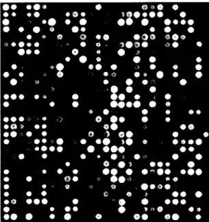
oligonucleotide microarray image show n in Figure 1.6 for A ffym etrix microarray.

A m ong these techniques, the high density oligonucleotide microarray technology

provided by Affmetrix G eneChip Com pany [8] has been widely utilized by thousands of

researchers because o f its high sensitivity and accuracy [9],

^^B K r^ T T jB ^ ^ H i j n ^^B n j ^ B |Bb bBh^B^BBF^B BEjl ^BBjQ j BJBBjBBB^Bb^^^B|| □ n B^B ^^BB H flE^BBmB^^B'J^Bj B^TjEBB^Bj^^Bfl ^Bfl • • • • • • • • • * • ■ • • » • r r r m B1^ ^ B |B Qj^B^^^BBETjB|^Bfl rT|^nBm ^^BESQBTj^B Q B E B E j m B B B D O O f j 9 | B B p G r^^B| V ] BBH f B B r ^ B | _{■ L M ^ ^ B} F V ] _{■ 3} • o • • • • 9 • • • • • • • • # » « • • •

• • •

• •

• • •

• •

•

(22)

6

Figure 1.6 Affymetrix microarray image

The microarray technique is originated from the Southern Blotting technology.

The Southern Blotting technique is mainly used in m olecular biology to detect a specific

sequence o f D N A in D N A samples. This technique has two important characteristics; one

is the transportation o f the DNA fragments, and the other one is the probe hybridization

o f the D N A fragments. In Southern Blotting, D N A strands are first cut into smaller

fragments by using restriction endonucleases. N ext, these tiny D N A fragments are

separated by size by gel electrophoresis method. A fter classification and separation, the

DNA fragments are transferred to a sheet o f nitrocellulose or nylon membrane. This

membrane is exposed to a single D N A hybridization probe with specific sequence. In

addition, this D NA sequence is labeled in order to be easily detected. A fter hybridization,

extra DNA fragments will be washed off. and hybridization fragments will be visualized

on film. In this way, the specific D N A sequence is detected.

Though the Southern Blotting is very effective for detecting the D N A special

(23)

method is that it is rather time consum ing and labor-intensive. Thus, microarray

technology is innovative, because it can manipulate and m ange thousands o f genes at the

same time. In 1995. the first DNA microarray was proposed for gene expression analysis

[ 1 0 ].

A co m m on microarray experiment contains the following six steps:

■ Experim ent preparation. Two samples are selected as the treated sample and the

untreated sample. For example, one sample is from a normal tissue, and the other

sample is from a tum or tissue.

■ Interest Nucleic acid separation and purification. For exam ple, the RNA

sequence for expression analysis or the D N A sequence for the comparisons.

■ Reverse transcription is performed to obtain the labeled sequence. For example,

the m R N A is reverse transcribed to cDNA. Also, a label is added in this process

through m olecular combination.

■ The c D N A sequence is mixed and hybridized in the solution. N ext, the mix is

denatured and spotted on a microarray, w hich could be a gene chip or a glass

microarray.

* The microarray is scanned by a special laser scanner, which can detect the label

quantitatively and qualitatively.

■ M icroarray image and raw data is generated after the scan process is performed.

1.3.1 cDNA M icro array

The cD N A microarray isolates the R N A sequence from both the control sample

(normal sample) and the experiment sample (diseased sample). N ext, it operates the

(24)

into cDNAs. After the reverse transcription, the cD N A s will be further labeled with

fluorescent probes, Cy3 for control sample and Cy5 for experiment sample. The Cy3 is in

a green channel with 530nm wavelength, and Cy5 is in a red channel with 630nm

wavelength [11]. W hen finishing the labeling process, c D N A microarray is scanned both

at the ~ 540nm and ~ 630nm for each channel correspondently. Two 16-bit monochromatic

images are generated after scanning, which are Red and Green images. In these two

images, each spot represents a specific gene [12, 13],

Normally, a cD N A experiment [13, 14] consists o f the steps illustrated in Figure

1.7.

tramcr*>*on,

l u t f M C t n f r t i b t M

«*** Cy3 {<><«**«}

Figure 1.7 cD N A microarray experiment from [13]

■ In the experim ent preparation step, the normal sam ple and the experim ent sample

are selected.

(25)

9

* In the reverse transcription step, the RN A sequences are reversely transcribed

into cD N A sequences.

■ In the hybridization and label step, the cD N A is labeled with a fluorescent dye.

Next, the labeled cD N A sequence is hybridized. A fter full hybridization, extract

D N A sequences will be washed away if they w ere not hybridized at all.

■ In the scanning step, the microarray will be scanned in the tw'o channels.

■ In the data extraction step, intensity data o f each spot will be extracted for the

subsequent analysis.

1.3.2 Affym etrix M icroarray

The Affymetrix microarray technique (Figure 1.8) is originated from late 1980s

by Stephen Fodor together with other scientists. Fodor at all introduced the sem i

conductor technique for biological setting in microarray fabrication process. This process

helped to construct a system to measure more and m ore various m R N A sequences in one

sample. In addition, Affymetrix microarray introduced small oligonucleotide sequences

(probes), containing 25-nucleotides located variously in their sequence com position. This

is an impressive characteristic compared to the cD N A microarray, which uses single and

long probes to detect the transcript o f interests because small probes could bring a better

discrimination between similar related transcripts over long oligonucleotides, especially

when m R N A s are highly abundant. Hence, w e mainly focused our research interests on

(26)

10

m m m

Figure 1.8 Affymetrix microarray chip from [12]

Probe sets are designed for each m R N A sequences [15]. Each gene normally

consists o f 11 to 20 different probes, which corresponds to a single transcript at different

locations. For Affymetrix microarray, it usually has tens o f thousands o f different probe

sets. This feature makes the Affymetrix m icroarray more desirable than cDNA

microarray, since it could allow scientists to monitor and m anipulate such am ounts o f

genes at the same time.

A nother significant characteristic is that Affymetrix introduces the Perfect Match

(PM) and the M ism atch (M M ) in a pair into the probes as shown in Figure 1.9. In other

words, each probe pair consists o f two probes, PM and MM. These two probes are

exactly the same, except for the one base in the middle. For exam ple, PM has 25-

nucleotides. which are perfectly hybridized to the m R N A sequences; whereas, M M has

the same 25-nucleotides, but there is only one base in the middle o f the 25 bases that is

(27)

11

In this case, false signals transcription caused from sim ilar com plete sequences were

completely eliminated, and M M was used to help scientists to learn and control the

unspecific signal and background signal.

m RNA reference sequence

5-probe set [

3

spaced probe pair

c : P M p r o b e M M p r o b e

I ___I

fluorescence intensity image

perfect m atch probe cells m ism atch probe cells

Figure 1.9 Probe level design in Affymetrix microarray from [16]

Normally, an Affymetrix experiment contains the following steps. This whole

process shown in Figure 1.10 usually requires two and a h a lf days:

■ First, the sample o f interest is selected.

■ Next, the R N A sequences are isolated. The R N A quality is monitored and

checked. After checking the quality o f R N A sequences, good quality RNA

sequences are labeled. These m R N A s experience the reverse transcription to

(28)

■ Next, this mixture is injected into the microarray platform. Hybridization is

performed on the gene microarray platform under specific temperature and

hours.

■ After com plete hybridization, the chip is scanned by a special laser, generating

the Affymetrix microarrav image in 16-bit gray level.

■ Finally, the intensity o f each pixel on the chip is recorded according to the

emission o f the fluorescent dye.

Total RNA cDNA

9iotiniabei*d cRNA A A A A A A A A A A A A Ravarsa Transcription In Vitro Transcription GcnoCWp Expression Array Hybridisation Fragmentation F ragm ented, / Biolifn-tabclod - B V cRNA B o

o

Wash and Stain -0v , _{Scan and} Quontltato

-O'"

Figure 1.10 Affymetrix microarray experim ent process from [17]

There are several microarray types developed by Affymetrix. T hey are different in

many aspects, such as different emphasis on genes, exons or genome wide transcriptions

(29)

13

The standard expression array is the most co m m o n array used in the public

research area, which could be canine, rat. human, fly, yeast, bacteria and plant. Such

probe arrays are available as public resources at U niG ene, G enBank. dbE S T and so on.

The microarray data for this dissertation mainly cam e from this standard expression array

database.

The exon array could provide the gene expression inform ation based on the exon

level. From this point o f view, the splicing patterns could be clearly monitored and

learned. It is known that not all the D N A sequence may be translated into a protein. After

generating the m R N A , there is an important step that rem oves the non-coding sections in

mRNA. These non-coding sequences are referred as to “introns.” The rest o f the exons

are constructed together in different ways resulting in various genes. This whole process

is called “splicing.” It plays a significant role in the h um an genom e system, because

different splicing and construction o f the exons will contribute to completely different

proteins.

The gene array contains more up-to-date genom e annotations for hum an and

mouse. Hence, it is more accurate com pared to the standard array. It is usually little

smaller than the standard array since it does not carry any m ism atch probes but the 5-

micron feature. This array is the next generation o f standard arrays. It begins to include a

large am ount o f perfect match probes for each gene and to drop all the mismatched

probes. Another impressive characteristic this array has is that it rem oves the 3 '-bias end

o f each transcript. Instead, it uses 26 different probes to cover the whole transcript.

Removing this 3 '-bias end will provide more accurate gene inform ation when alternative

(30)

14

The tiling array only covers several organism s such as human, m ouse and yeast.

The tiling array uses 25-m er probes which are evenly located every 35 bases with around

10 bases as the gap between each probe. It only uses the evenly located probes on the

non-repetitive part o f the genom e sequence rather than using the probes which

corresponds to the relevant gene expression sequences. This type o f array is widely used

(31)

CHAPTER 2 INTRODUCTION OF AFFYMETRIX MICROARRAY IMAGE

O ver the last decade, the microarray biotechnologies have becom e increasingly

important in the biomedical research field, since they are capable o f monitoring the

expression levels o f thousands o f genes simultaneously. This quality o f the technology

that allows researchers to access such a large num ber o f genes simultaneously while the

traditional m ethods are limited in the num ber o f genes that can be researched at one time,

sparked the interests o f scientists in researching and im proving their understanding of

genomic regulation and gene interaction. The D N A m icroarray technology has provided

the scientific com m unity with a tool to be used in understanding the basic aspects o f life

development and especially in exploring genetic causes and anom alies occurring in the

human body.

The microarray applications currently are very wide; one o f the first applications

o f microarravs was genom e sequencing analysis using hybridization, tissue microarrays

used in the study o f cancer, including the molecular profiling o f tu m o r specim ens and of

the applications determining gene copy number. Drug discovery is one o f the largest

aspects. The m icroarray's capabilities make them a perfect candidate for various stages of

drug discovery, validation and clinical studies. O ther applications o f microarrays are in

DNA computing, bioinformatics, and data mining, where the m icroarrays are required

(32)

16

tools for solving com putational problems, analyzing huge am ounts o f data with similar

characteristics, by using diverse analytical methods: B ayesian methods, neural networks,

clustering, multivariate statistical analysis, and information retrieval [18].

Last, but not the least, and the direction where ou r interest lies was the gene

expression analysis, with the goal o f gene discovery and the possibility o f using these

results in monitoring and detecting the changes in gene expression from different cells.

There are already chips with arrays o f many types o f genes such as hum an or species like

rat. mouse and Escherichia coli and more. The Affymetrix Com pany m anufactures chips

for analysis o f D N A microarrays, chips that scientifically match significant parts o f

human and non-hum an genomes.

The method developed in this dissertation aim ed to provide a better segmentation

method compared to the ones currently used. We expected that the im provement could

lead the way to a quantitative feature o f the D N A arrays. Such results would impact

directly the many fields that use D N A arrays; the most im portant impact will be in a

better prediction o f genes that activate different diseases. We looked to provide a stepping

stone towards quantitative results from D N A array experiments (at the mom ent we

receive rather qualitative signals o f the gene-disease relationships from such

experiments). With the advancem ent o f the hardw are in digital photography and the

processing/manipulation o f cells, w e fully expected the im ages obtained after the DNA

arrays experiments to reach much higher resolutions and have significantly lower noise in

the signals and. thus, the proposed algorithm to lead to dramatic im provem ents as

opposed to the currently used Affymetrix segmentation method. This new method will

(33)

17

light on the cellular processes. This segmentation o f a picture is one o f the three

important steps in microarray image processing, together with spot gridding and

information extraction. It directly affects the accuracy o f gene expression analysis in the

data mining process that follows [19, 2 0 , 2 1 ,2 2 ],

2.1 Overv iew o f A ffym etrix M icroarray Im age A nalysis M ethods

In a microarray experiment, the image analysis could be view ed as one o f the

most crucial steps o f processing, which could have a large impact on the subsequent data

analysis, such as clustering or identification o f different gene expression levels. During

the microarray experiment process, usually two samples o f (a healthy sample versus

diseased sample) microarravs are hybridized with com plem entary D N A labeled with

usually two different fluorescent dyes, Cy3 and Cy5. N ext, the hybridized microarrays

are processed by a microarray scanner to visualize the red and green florescence. In other

words, the hybridized microarrays are imaged at each spot. In this w ay, a raw 16-bit TIFF

image is obtained. The florescence intensity o f each spot represents the hybridized level

o f the sample. Therefore, analyzing the microarray image is one o f the most important

steps in a microarray experiment. The microarray image analysis can be described as a

three step process [ 11].

The addressing or gridding step is perform ed to find the exact location o f each

spot and to assign the coordinates to each spot. The purpose is to define the spot region

based on the microarrav image layout information. After gridding on the microarray

image, each spot is assigned with a geometric location, w hich is a square or a rectangle.

T he center o f each spot and the region between the center and the boundary are used to

(34)

misalignment usually happens. For example, the m icroarray chip may not be arranged

exactly in the center during the scanning process. Or the sub-array chip m ay be shifted

subtly during the hybridization process. All these issues will be considered and handled in

our image analysis process [23].

The segm entation process was the main concern in our research. In the data

acquisition process, the segmentation o f spots is the one o f the m ost challenging tasks

and has a significant impact on the gene expression analysis process that follows. The

task is to identify the pixels either as foreground (within the printed spot) or as

background (beyond the printed spot). In this sense, the image segm entation is a process

that divides an image into two mutually exclusive regions: foreground and background.

The key point at this stage is to get the exact shape o f the foreground pixels. This

exactness does not usually happen in the previously used segmentation methods in the

literature. In this way, the foreground and the background regions are classified and the

tlorescence intensity for the spot is calculated according to this classification.

However, the microarray images are hard to segm ent since they have highly

varying image contrast different from experiment to experiment and also contain a high

level o f background noise and image artifacts. The segmentation step is further

complicated by the non-uniform shape and surface intensity distribution in the

experiment pictures.

The intensity extraction follows next. The value o f each pixel represents the

expression level o f hybridization for that specific D N A sequence. H ence, the next step in

processing D N A arrays is to calculate foreground tlorescence intensity, background

(35)

19

some other calculations are performed such as the possibility o f random hybridization,

noise and quality measures. Many methods use the mean or the median pixel value as the

whole value o f the foreground spot mask. Additionally, these m ethods make use o f the

statistical tests to measure the background intensities relative to the foreground

intensities, [11, 24], Therefore, the result produced in the segm entation step is extremely

important in the subsequent image analysis process.

In recent years, several methods have been developed to segm ent microarray

spots and have been incorporated into com m ercial m icroarray im age analysis software

p a c k a g e s [25, 26].

The last step o f the process is the intensity to gene expression signal value step.

The intensity only represents the abundance o f hybridization for target interested

sequence in each spot, not for each gene. The last step is to sum m arize the intensity

values into the signal value, which represent the expression level for each gene.

2.2 A ffym etrix M icroarray Im age A nalysis Process

In Affymetrix, all microarray im age analysis is accomplished in Gene Chip

Operating Software (G C O S ) produced by Affymetrix Company. It provides a set of

com prehensive analysis tools for data m anagem ent and control in the processing of

microarrays. The software summarizes all the probe intensity values and com bines them

into gene signal values after image gridding process. Besides these characteristics, this

software enables data analysis to be customized, autom ated and integrated with various

laboratory systems.

First, segm entation and intensity extraction are performed by the built-in GCOS.

(36)

2 0

the experiment design. After identifying the position o f each probe, G C O S omits the

outer boundary pixels. Only the inner pixels are included and considered to be within the

foreground area. The method chooses the 75 th percentile o f the rest o f the pixels in the

square to represent the intensity for each probe. Table 2.1 is the pixels matrix o f one spot

in microarray image.

The outer highlighted pixels are dropped o ff in Table 2.1. The 75th percentile of

remaining inner pixels is recorded as the intensity value for the spot. The reason why

GCOS omits the outer pixels is that it is believed that such pixels are not reliable and may

carry some noise and errors, for they may be located by the m isalignm ent in the scanning

process, or they may be influenced by the neighboring probes which have large amount

o f emission. These intensity values are recorded into the C E L file.

Table 2.1 Pixels matrix for one cell

196

369 " 279 ' 458 219

f g

m 166 : 241 286 451... g g

In Affymetrix, G COS chooses the 7 5 lh percentile o f the interior pixels o f each

probe cell as the intensity for each probe. Research from Harry Zuzan [23] shows that

with the increasing o f the pixel values, the variance w'ould becom e unstable when

choosing the 75th percentile as the probe intensity. In addition, this m ethod is not robust

enough when dealing with different qualities o f cells. Hence, in this dissertation, we

introduced an intensity extraction algorithm named as “ Segmentation Based Contours”

(37)

detect a curve which is constrained in a specified image without any gradient calculation

but minimizing the energy based function. Thus, the A C W E presented by Tony F. Chan

and Luminita A. Vese [27] has more advantages in finding objects within a microarray

image in which boundaries are not defined by gradient. We will present more details for

this ACW E m ethod and its modified method SBC.

Next, intensity values for each spot are com bined transformed into the gene

expression signal value. The Affymetrix G C O S software uses the M A S 5 algorithm to

calculate the signals from intensities [28, 29, 30], The Genechip array designed by

Affymetrix Com pany is the probe level design array. A G enechip array contains many

probe cells, where each probe cell is related with a specified target sequence probe. Probe

spots are tiled into probe pairs with a Perfect M atch (PM ) and a M ism atch (MM). There

is only one base in the middle changed in M M sequence, where it does not follow the

com plement rule. All related PM and M M together consist o f a probe pair, related to a

whole expressed gene transcript shown in Figure 2.1.

1 2 3 4 5 6 7 PM MME1 1 1 S3 1 1 3 8 ■ 9 1 0 m c e II ■ p ro b e s e t pro b e p a r

Figure 2.1 Probe set from [28]

Before calculating the signals, the M A S5 conducts global background subtraction

and noise correction based on the raw intensities in C E L file. This background adjustment

noise correction could even out the background errors caused by different cell locations.

(38)

distance d k is com puted between the chip coordinate (x, y ) and the center o f each sub

zone. Next, the weighting factor Wk is obtained based on d k .

W k ( x ,y ) = (d \ { x , y) + s m o o t h ) * 1, s m o o t h = 100. (2.1)

r

Figure 2.2 Background subtractions from [28]

Based on such distances d k and W k together and a constant b, a weighted sum is

obtained, which is used for each probe cell ( x , y ) .

b( x, y ) = Z b Z k W k (x, y ) . (2.2)

Now, M AS5 com putes the adjusted intensity value by shifting the original

intensity value down based on the local background/). T h is/) is considered to be the

noise correction. For noise correction, local noise factor n is obtained based on the

standard deviation in each sub zone.

(39)

23

Next, an initial threshold and a floor are specified such that no adjusted intensity

value is below that threshold. The adjusted intensity is calculated from subtracting this

local background.

A ( x , y ) = m a x ( / ' ( x , y ) — b ( x , y ) , N o i s e F r a c * n ( x , y ) ) ,

w h e r e / ' ( x , y ) = m a x ( I ( x , y ) , 0 . 5 ) , N o i s e F r a c = 0.5. (2.4)

After adjusting the background for each cell, the M AS5 algorithm uses the new

intensities to calculate the signal for each probe as follows:

1. An ideal m ism atch value is calculated and subtracted to adjust the PM

intensity. Tbi is the one step biweight algorithm. In an Affymetrix microarray, the reason

why it introduces the M M probe is that it com prises the background noise and cross

hybridization, which will bring impact on the PM probe. Hence, the ideal possible MM

value should be less than PM value. However, in som e cases, the M M value is larger than

PM value. This result indicates that this M M value is a physical impossible measurement.

It cannot be used to calculate the signal value. Instead, an adjusted value should be

estimated based on the whole gene probe set level. M A S5 uses the one step biweight

algorithm to calculate this specific background estimation S£?j.

SBi = T ^ l o g P M i j - l o g M M i j ) , } = 1 , 2 , . . . ^ . (2.5)

The one-step biweight algorithm begins by calculating the m edian M for a data set

w ith n values. In the signal measurement, this data set consists o f the l o g ( P M — 1M)

probe values o f a probe set. Next, we calculate the absolute distance for each data point

from the median, and calculate S. the median o f the absolute distances from M. The

(40)

2 4

For each data point i, a uniform measure o f distance from the center is given.

(2.6)

Next, calculate the w eight by the bi-square function.

(1 - u 2) 2, \u\ < 1,

0, |u | > 1. (2.7)

Finally, the corrected values can be calculated by the one-step u-estim ate.

(2.8)

If the background estimate S B; is large, the related values in the probe set are

reliable. This S B t is capable o f constructing the ideal adjusted m ism atch I M if necessary.

If SBi is small, more o f PM values are used to calculate the ideal adjusted mism atch IM.

These different cases which determine the ideal adjusted m ism atch I M are described as

follows:

When M M value is less than PM value, this M M provides a reliable estimation

for the probe background. W hen M M value is not less than PM value, this M M value is

not reliable, but still provides some relevant information for the probe. If SBi is less than

or equal to 0.03. the M M value provides the least inform ation estimation.

2. The adjusted P M intensities are log-transform ed to stabilize the variance.

Given the adjusted ideal mism atch MM, probe value (PI') is calculated with the

numerical stability. MM[j, w h e n MM!y- < PMLj, M i j = < r M • • -^s b~, w h e n MMj j > P M itj a n d S B t > 0.03, , w h e n M M y > P M tj a n d S B t < 0.03. T( ; = m a x { PMi j — I M i j . D ' ) , w h e r e D = 2 20. (2.10)

(41)

25

Next, log-transformation is performed on probe value for each probe cell.

PVltj = \ o g ( y i:j), j = (2.11)

Absolute expression value for each probe set is obtained by perform ing the one

step biweight estimate algorithm.

S i g n a l L o g V a l u e — ^ ( P Fi l f ..., P Vi n ). (2.12)

3. The biweight measurem ent is used to calculate the robust mean o f the input

values. Signal is output as the anti-log o f the Signal Log Value. Finally, the reported

signal for each probe set is obtained.

R e p o r t e d S i g n a l = n f x s f x 2 SignalLogValue. (2.13)

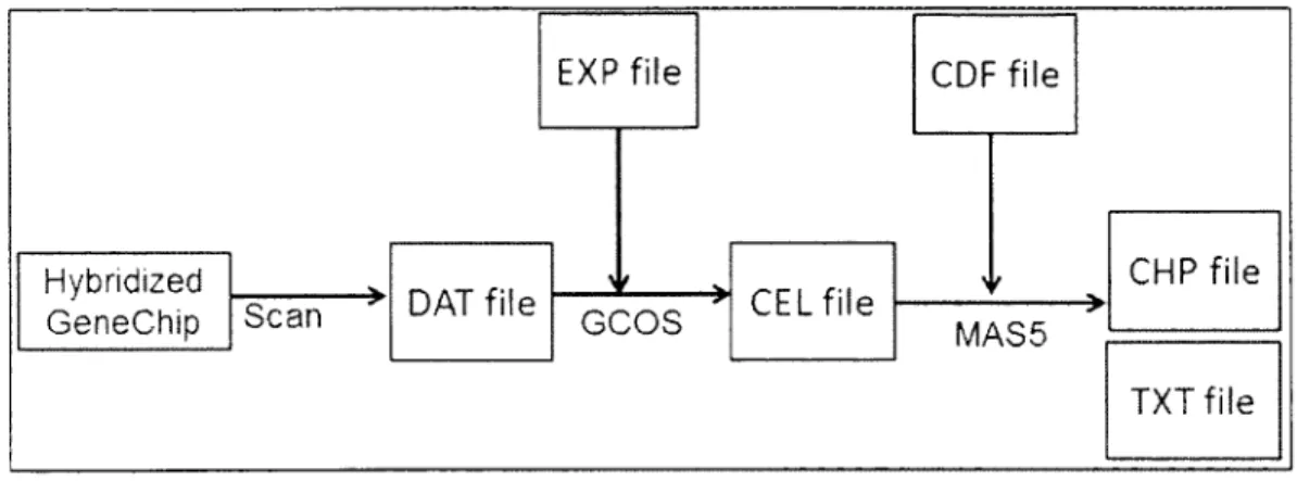
2.3 A ffym etrix M icroarray Im age A n a ly sis Flow in G C O S

After finishing the microarray experiment, the m ost crucial step is to extract most

reliable data information from the microarray image, obtaining the intensity value for

each probe on the chip. The probe intensity is the foundation o f the whole microarray

image analysis because all the subsequent data analysis is based on the probe intensity

value, calculating gene expression signals and so on. Thus, how' to achieve more accurate

probe intensity values was our main research interest. For Affymetrix microarray image,

all such analysis was accom plished in GCOS. Figure 2.3 is the G C O S m icroarray image

analysis flow' chart. The gene chip was scanned after m icroarray experiment. The raw

image information was stored in DAT file and we used G COS to open this DAT file.

Alignment gridding was automatically performed and intensity values were written in

CEL file. W hen the intensity values were obtained, G C O S im plem ented the MASS

(42)

2 6

for each probe set. This gene signal value was stored in C H P file and T X T file. One was

in special format in C H P file. The other one was in text form at in T X T file.

EXP f i l e CD F f i l e

TX T f i l e

Figure 2.3 G C O S microarray image analysis flow

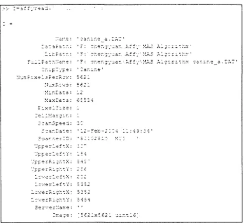
The DAT file shown in Figure 2.4 contains the data inform ation o f raw 16-bit

(TIFF) optical image followed by the relevant header information show n in Table 2.2. It

also includes that array chip layout information and experim ent information, etc. The

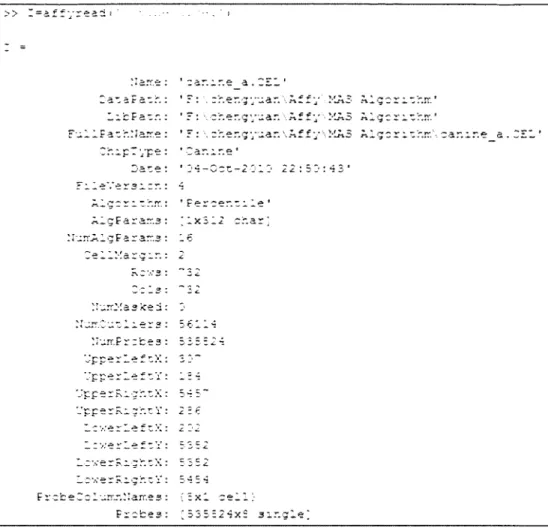
CEL file show n in Figure 2.5 contains the information for each probe cell. It includes the

layout coordinates o f each cell, the intensity value for each cell, the num ber o f pixels

included for each cell and the standard deviation o f each cell, etc. It is written in a special

(43)

2 7 X a r . r : * r a r . i r . e 2 a 7 a F a i r . : ’ F : r r . a r . L i r F : 1 F : ; r . s r . 1 Fa ~ r . Xa r r . e : * r : c r . e r . C r . i p T y p e : ' : r e 1 i x r l 3 r * r R : v ; : 5 € 2 1 v;3 : a * ■ t X i r X a t a : 1 2 M a x D a ~ a : c = : 2 4 ? i x e l ! : 2 e : 1 l e l l M a r g i i r . : 1 F r a r . S p - e d : 2 1 F j a r . T a t e : ‘ 1 2 r e f c -S c a r . r . e r i r - : ■ s : 1 - 2 = : V c r e r l e r r X : - 1 : - ; •: Y p p e r R i j ' t i X : = 4 : ~ V p p e r K : : ' : :: 2 2 € Icv.'-e r L e f d X : <. . ^ 1 " v : e r l e f " Y : 5 3 5 2 L c v e r R i - j r . t X : 5 2 5 2 l c v ; e r r i c r x Y ; 5 4 5 4 S e r v e r X a r r . e : Zrr.a -5® : ; 5 € 2 1 x £ 6

Figure 2.4 DAT file structure shown in M ATLAB

Table 2.2 Part o f header information for DAT file

Index Description Type

1 Type o f file, must be OxFC. BY TE

2 N um ber o f pixels per line. W O RD

3 N um b er o f lines in the image. W O RD

4 The total num ber o f data points (pixels) in the image. D W O RD

5 M inim um pixel value in the image. D W O RD

6 M axim um pixel value in the image. D W O RD

7 Mean pixel value. double

8 Standard deviation o f the pixel values double

9 N um ber o f pixels per row (padded with spaces), preceded with

"CLS=."

char[9]

10 N um ber o f row s in the image (padded with spaces), preceded

with "RWS=."

(44)

28 a£f vr eaS« >> "IT. 5 A1 g c z'r. rr.\ . er.g * V e r s MurrJMasJcei e r a :Iurr.Fr z f c s s f *:X rc>; '.s' 5 T r*. -eve rr.ighc: F r c f c e C o l uir_-.!! a rr. e 3 F r o b e s c e l l :■ l e x : s i r . g l e

(45)

T a b l e 2 .3 P a r t o f f o r m a t d e s c r i p t i o n f o r C E L file

2 9

TAG Description

Version The version number. Alw ays set to 3.

TAG Description

Cols The num ber o f colum ns in the array ( o f cells).

Rows The num ber o f rows in the array (of cells).

TotalX Same as Cols.

Total Y Same as Rows.

OffsetX N ot used, always 0.

OffsetY N ot used, always 0.

G ridCornerU L XY coordinates o f the upper left grid corner in pixel

coordinates.

G ridCornerU R XY coordinates o f the upper right grid corner in pixel

coordinates.

G ridCornerLR XY coordinates o f the lower right grid corner in pixel

coordinates.

G ridCornerLL X Y coordinates o f the lower left grid corner in pixel

coordinates.

Axis-invertX N ot used, always 0.

Axis-invertY Not used, always 0.

swapXY N ot used, always 0.

The CDF file shown in Figure 2.6 contains the inform ation for each probe set

gene. It includes the num ber o f probe sets, the nam e o f each gene pro b e set, the number

o f probe pairs o f PM and MM. and the coordinates for each probe pairs, etc.

The CHP file shown in Figure 2.7 contains the experim ent results created from

CEL and C D F files. It includes the gene expression value for each probe set and includes

(46)

30

>> : = a:fyreaa i ' ■ : =

:!d.T.a : ' Car.ir.e a . rdf ' Cr.ipType: ’ Car.: re a ‘

IcfcPacr.: ' F : \ cr.er.gyj.ar. f.ffyXWir.” xp sr.are\2-.2XF '

FallFacr.'.’air.e: ' F: \ rf.er.gyaar.'. Af fy'-.Wir.” xp share\ACKE\ Car.ir.e a. c a t’

t a - e : ' 23-5ep-2 1 e : '

1 ) U» ” 3 2 2c 13 : “32 Uujr.FrcfceSets: 23213 Xurr.'CFr cbeSecs: 9

frifceietCclu rr.r.' larr.fts: •:€xl cell;

Frcfc»S*'.s: ; 23 92 2 xl scrucc;

Figure 2.6 CDF file structure shown in M ATLAB

; a r . ' A f £ y \M A 5 A l5c n . c l - . r r . ’ - a r . \ A f f y \ MAS A l e e r 1 c err. ’ c a r / ' A f f y \ M A 3 Sac a.Pach: L r r F & c h : r c t r . ' i a r . e : nncr.rr.''- car. 1 I h r p . y p e : A-sayType: 1 =t c e : Sxpr^s^icr.Scac ' A l c F a r a r r . ® : 11 ur . T h r p S u ; : m r y : 1 x 1 = 3 c h a r IJcrr.FrchaSecc IMr.lCFnbeSera F n ’c e S e c . ?

Figure 2.7 CF1P file structure show n in M ATLAB

The T X T file is the text format o f C H P file, w'hich contains the sam e information

as the CHP file. The EXP file is the text file, w hich contains the experim ent details, such

(47)

CHAPTER 3 MICROARRAY IMAGE SIMULATION METROD

The Affymetrix GeneChip microarrays have becom e a crucial com ponent o f gene

expression and genotype research for m any laboratories. D ata analysis remains a major

challenge for the effective use o f GeneChip data. There is high interest in analyzing the

microarray data and improving in the existing analyzing methods.

We will com pare our proposed segm entation m ethod SBC with the method

currently used by the Affymetrix. The Affymetrix G eneC hip Operating Software (GCOS)

is an operating system that controls A ffymetrix instruments, acquires data, and executes

gene expression analysis. In addition, G C O S contains an em bedded database that

manages both experim ent information and data. The com parison will not be made in

respect to the segmentation time, the Affymetrix m ethod is by far m uch faster than our

method, and it will concentrate on performance, in the number o f genes that can be

detected. We planned to run an experiment to detect active expressed genes in different

organisms. Since the experiment involved detecting g e n e s ’ expressions, even a small

improvement in the detection rate could be crucial in determining a gene o f interest.

However, due to the lack o f the "ground true inform ation.” it was difficult to

evaluate different intensity extraction algorithms. Therefore, we utilized an advanced

(48)

kinds o f segmentation analysis algorithms. It contained all the experiment and

manufacture steps for producing one microarray image in practice. It also embraced

biological realistic characteristics, which could affect the microarrav image quality

significantly. The most im portant thing is that this model could provide the "ground true

information" to help us have a deep understanding on h o w the algorithm performs. The

simulation program can be dow nloaded from [32], In order to simulate data carrying real

genetic information, we used the analyzed intensity o f real Affymetrix microarray images

as data input obtained from GCOS for the simulation model.

In this chapter, we will present the data input used in the simulation model and the

description o f this simulation method.

3.1 D atabase for Sim ulation M odel

The original Affymetrix microarray images can be dow nloaded from [33]. All the

data on this website are the sample test data provided by Affymetrix C om pany as a free

test online source. Some o f those data are not available, Canine2.0, Chicken. Citrus,

Cotton, Dros Test Yease, Focus-Ecoli, H G -U 133, M G -U 74, M ouse 430, etc. In our

research, w'e utilized eight different high resolution microarray im ages from [33 ] as the

(49)

Table 3.1 Data sets for simulation model

Bovine_a: A replicate probe array file for the Bovine G enom e Array.

Bovine_b: A replicate probe array file for the Bovine G enom e Array.

Canine_a: A replicate probe array file for the Canine G enom e Array.

Canine_b: A replicate probe array file for the Canine G enom e Array.

Vitis_a: A replicate probe array file for the Vitis Vinifera (grape) G enom e Array.

Vitis b: A replicate probe array file for the Vitis Vinifera (grape) G enom e Array.

Yeast_a: A replicate probe array file for the Yeast (Y G-S98) S98 G enom e Array.

Yeast_b: A replicate probe array file for the Yeast (Y G-S98) S98 G enom e Array.

Bovine_a and Bovine b are all selected from Bovine genom e. This Bovine

genome array can be used to understand over 23,000 Bovine transcripts. This array is an

idea microarray chip for scientists to study cattle. Researchers are able to monitor genetic

mechanisms, which regulate different kinds o f traits such as disease resistance, m eat and

dairy production, stress tolerance and so on.

C anine_a and Canine_b were selected from the Canis fam ilies’ genome, which is

an important model organism used for hum an disease study in the biom edical field. This

Canine array enables researchers to interrogate 18,000 Canine genom es m R N A /EST

transcripts and 20,000 non-redundant predicted genes simultaneously.

Vitis_a and Vitis b were selected from the Vitis genome. This Vitis genom e array

is the first array to provide com prehensive analysis for V. vinifera genom e and is

provided as free sample test data from the Affymetrix database. There are sixteen pairs

for each oligonucleotide probe set to measure the specific sequence o f target genes. All

sequence o f target genes were selected from G enBank, dbEST. and RefSeq online gene

sequence research databases.

Y east-1 and Yeast-2 were selected from the Yeast genome. This genome array

(50)

34

Saccharomyces cerevisiae and S chizosaccharom yces pombe. It provided the

comprehensive coverage for these two species, including around 5,744 probe sets for

5,800 genes in S. cerevisiae and 5,021 probe sets for all 5,031 genes in S. pombe.

In Affymetrix, all these array files were provided in DAT file format. The

researcher needed to dow nload G COS to open this DAT file format. N ext, the raw

microarray image will be shown in G C O S platform. The G COS autom atically allocated

the grid alignm ent information from DAT file. The intensity value for each spot cell was

analyzed and stored in the CEL file. W hen the intensity value was obtained, the

researcher was capable at calculating the gene signal value by using the build in MAS5

algorithm, recorded in CH P file. The G COS platform is show n in Figure 3.1.

&] 1:3 ? G c r t t C i r t p O p e r a t i n g S o f t w a r e Pun T 0(.‘rC ’.-Vrfi-jow H*;'p m Short*, Figure 3.1 G C O S platform

(51)

35

3 .2 M i c r o a r r a y S i m u l a t i o n M e t h o d

In order to com pare the segmentation results from the two m ethods SBC and

Affymetrix G C O S, we introduced an advanced Affymetrix microarray image simulation

model. This simulation model played a significant role in validating different kinds of

segmentation analysis algorithms, since it contains all the m anufacture steps for

microarray image. This model em braced biological realistic characteristics which could

affect the microarray image quality significantly. M ost important thing is that this model

could provide the "ground true information" which led us have a deep understanding on

how the segm entation algorithms perform.

The simulation model contained six main steps w hich are slide manufacturing,

data input, biological noise, slide hybridization, slide scanning and im age reading (Figure

3.2). By operating the model parameters, the sim ulation process will provide three

different qualities images, which are high, normal and bad quality.

D ata — ► B io lo g ica l n o i s e — ► Slide m a n u f a c tu r i n g a n d - - - ► S lid e s c a n n i n g - - - ► I m a g e r e a d i n g h y b rid izatio n

Figure 3.2 Simulation steps

Data input for the Affymetrix microarray image is the intensity for each cell in the

microarray chip. In addition to the intensity data, the cell location, probe name and

location and their identifiers should also be specified in a proper format by using a file

input module. The requirem ent for the input data format is described in Table 3.2. In our

research, w e used the analyzed intensity data obtained from real A ffym etrix microarray

New microarray image segmentation using Segmentation Based Contours method

Louisiana Tech University

Louisiana Tech Digital Commons

Doctoral Dissertations

Graduate School

Winter 2013

New microarray image segmentation using

Segmentation Based Contours method

Yuan Cheng

Follow this and additional works at:

https://digitalcommons.latech.edu/dissertations

Part of the

Applied Mathematics Commons

,

Applied Statistics Commons

,

Biomedical

NEW MICROARRAY IMAGE SEGMENTATION USING

SEGMENTATION BASED CONTOURS METHOD

OCTOBER 31, 2012

y

ABSTRACT

APPROVAL FOR SCHOLARLY DISSEMINATION

TABLE OF CONTENTS

66

LIST OF TABLES

2

21

LIST OF FIGURES

ACKNOWLEDGEMENTS

CHAPTER 1

INTRODUCTION OF DNA AND DNA MICROARRAY

building block of DNA

phosphate

sugar

i'

G

sugar

base

(G

phosphate

nucleotide

• • •

• •

•

• •

• •

•

o

-O'"

CHAPTER 2

INTRODUCTION OF AFFYMETRIX MICROARRAY IMAGE

196

f g

CHAPTER 3

MICROARRAY IMAGE SIMULATION METROD