Exploring nonlinear regression methods, with application to association studies

(1)

Exploring Nonlinear Regression Methods,

with Application to Association Studies

Douglas Christopher Speed

St Catharine’s College

A dissertation submitted to the University of Cambridge

for the degree of Doctor of Philosophy

Department of Applied Mathematics and Theoretical Physics, Centre for Mathematical Sciences,

Wilberforce Road, Cambridge, CB3 0WA,

United Kingdom.

(2)

(3)

To my Parents.

With special thanks to Simon, Marion, Christina, Radhika, Shamith

and everyone who helped me out.

(4)

This thesis is the result of my own work and includes nothing which is the outcome of work done in collaboration except where specifically indicated in the text.

This thesis has been typeset in 12pt font using LA_TEX2_ε _{according to the specifications}

(5)

September 30, 2010 Douglas Christopher Speed St. Catharine’s College

Exploring Nonlinear Regression Methods, with Application to Association Studies

The field of nonlinear regression is a long way from reaching a consensus. Once a method decides to explore nonlinear combinations of predictors, a number of questions are raised, such as what nonlinear combinations to permit and how best to search the resulting model space. Genetic Association Studies comprise an area that stands to gain greatly from the develop-ment of more sophisticated regression methods. While these studies’ ability to interrogate the genome has advanced rapidly over recent years, it is thought that a lack of suitable regression tools prevents them from achieving their full potential.

I have tried to investigate the area of regression in a methodical manner. In Chapter 1, I explain the regression problem and outline existing methods. I observe that both linear and nonlinear methods can be categorised according to the restrictions enforced by their underly-ing model assumptions and speculate that a method with as few restrictions as possible might prove more powerful. In order to design such a method, I begin by assuming each predictor is tertiary (takes no more than three distinct values). In Chapters 2 and 3, I propose the method

Sparse Partitioning. Its name derives from the way it searches for high scoring partitions of

the predictor set, where each partition defines groups of predictors that jointly contribute towards the response. A sparsity assumption supposes most predictors belong in the “null group” indicating they have no effect on the outcome. In Chapter 4, I compare the

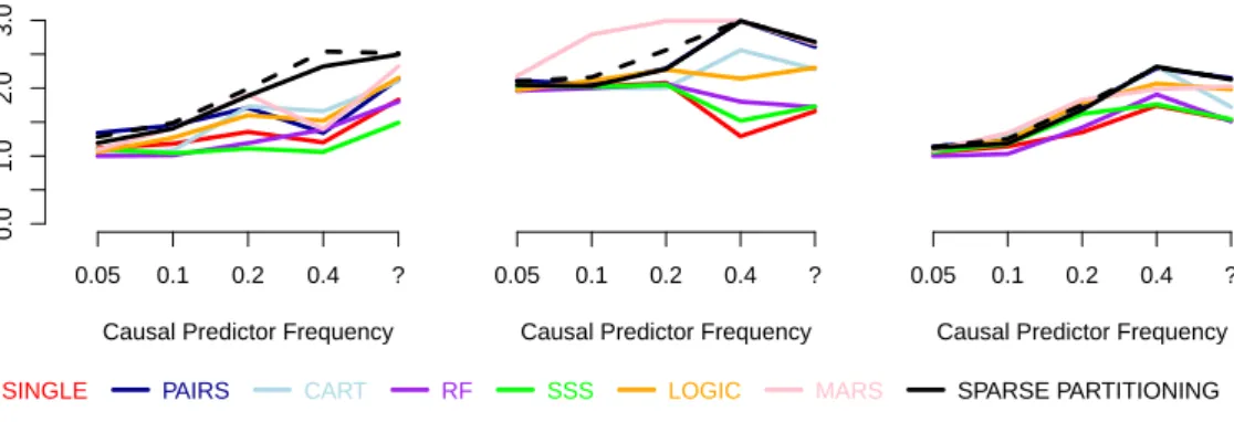
perfor-mance of Sparse Partitioning to existing methods using simulated and real data. The results

highlight how greatly a method’s power depends on the validity of its model assumptions.

For this reason, Sparse Partitioning appears to offer a robust alternative to current methods,

as its lack of restrictions allows it to maintain power in scenarios where other methods will fail.

Sparse Partitioning relies on Markov chain Monte Carlo estimation, which limits the size of

problem on which it can be used. Therefore, in Chapter 5, I propose a deterministic version of the method which, although less powerful, is not affected by convergence issues. In Chapter 6,

I describeBayesian Projection Pursuit, which adds spline fitting into the method to cope with

(6)

(7)

Glossary of Symbols

Below is an outline of the notation I use throughout this thesis. Data Variables

n - number of samples, indexed by the variable i.

N - number of predictors, indexed by the variable g.

X - predictor matrix (size n×N).

Y - response vector (length n).

Subscripts are used to indicate particular elements of a vector or matrix.

Negative subscripts indicate a vector/matrix with those elements removed. Regression Equation

l(_E(Y)) =f(X) - l is the link function, while f is the underlying relationship.

Partitioning Notation

G={G0, G1, . . . , GK} - a partitioning of (up to C copies of) {1,2,. . . ,N}.

The null groupG0 indexes predictors not associated,

G1, . . . , GK index groups of at most S associated predictors.

I = (I1, I2, . . . , IN) - alternative representation ofG.

Ig ∈ {0,1, . . . , K}denotes to which group predictor g belongs.

f ={f1, f2, . . . , fK} - functions acting on each non-null group.

SI lists the associated predictors: g ∈SI ⇔Ig 6= 0.

[I] denotes an equivalence class of partitions: I0 ∈[I]⇔SI0 =SI.

The underlying relationship is modelled asf(X) =f1(XG1) +f2(XG2) +· · ·+fK(XGK).

Projection Pursuit

ξk = (ξk1, ξk2, . . . , ξkN) - direction coefficients for the kth group.

Υ= (Υ1,Υ2, . . . ,ΥN) - condensed representation ofΞ ={ξ1,ξ2, . . . ,ξK}.

Can merge ξ1g, ξ2g, . . . , ξKg → Υg, as at most one is non-zero.

The projection pursuit model is f(X) =f1(Xξ1) +f2(Xξ2) +· · ·+fK(XξK).

Miscellaneous

P() denotes a probability mass/density function of the random variable.

(8)

List of Abbreviations

Below are some abbreviations and phrases I use more than once in this thesis. Regression Methods

Single - Tests each predictor individually for association (my own implementation).

Pairs - Tests all pairs of predictors for association (my own implementation).

CART - Classification and Regression Trees (Breiman et al., 1984).

RF - Random Forests (_Breiman, 2004).

SSS - Shotgun Stochastic Search (_Hans et al., 2007).

Logic - Logic Regression (Ruczinski et al., 2003).

MARS - Multivariate Adaptive Regression Splines (Friedman, 1991).

Genetic Terms

SNP - Single nucleotide polymorphism - a single base pair mutation.

LD - Linkage disequilibrium - the tendency of nearby genetic variants to exhibit

strong correlations, due to being frequently inherited jointly through generations. Mathematical Terms

MCMC - Markov chain Monte Carlo - A stochastic technique for sampling from a posterior distribution when explicit calculation is not (readily) possible.

δ{a} - The delta function - a point mass function at a, whose integral is defined as 1.

1(·) - The indicator function which takes value 1 if and only if its argument is true.

U(a, b) - A uniform distribution on the interval [a, b].

β(a, b) - A Beta distribution with shape parameters a and b.

B(a,b) - The Beta function, the normalising constant of the Beta distribution β(a, b).

N(a, b) - A normal distribution with mean a and variance b.

φ(a) - The probability density function of the standard normal distribution _N(0,1).

Φ(a) - The cumulative density function of the standard normal distribution _N(0,1).

Link Functions

Logit(a) - The logit function, equal to log(a/(1−a)) - a commonly used link function

which maps a probability to a real value.

Probit(a) - The probit link function, equal to Φ−1₍_a_{), the inverse cumulative density}

(9)

Overview of Sparse Partitioning Algorithms 0 1 0 ... 2 1 1 2 0 ... 0 0 0 2 ? ... 1 2 2 0 ? ... 0 2 2 ? 0 ... 2 1 0.3 -5.0 9.1 ? 0.5 0 ? 1 1 0 Predictors X Tertiary (0, 1, 2) M C M C S A M P L I N G

BASIC PREPROCESSING OF X &Y

Sampling Stage 3 (Probit Link) Sampling Stages 1 & 2 Sampling Stage 4 (Projection Pursuit) Sample Missing X, Y & Predict Y

POSTERIOR ESTIMATES OF ASSOCIATION Response Y Continuous / Binary 3.9 ... -1.5 -4.8 ... 8.8 0.5 ... 2.3

-1.3 ... 3.2 3.2 ... -1.2 Confounding Cofactors © (Tertiary) (Any) .. . .. . ... ... ... 0 ... 0 1 ... 2 0 ... 1

2 ... 1 1 … 2 .. . Or ONE-PREDICTOR-AT-A-TIME TESTS BASIC PREPROCESSING OF X &Y

BASIC PREPROCESSING OF X &Y

Input Parameters Sampling Stage 1+2 M C M C S A M P L I N G Better Model? Y E S DETERMINISTIC VERSION N O .. . .. . .. . ... ...

Three are three Sparse Partitioning algorithms. Solid lines indicate steps involved in the

original version, dotted lines refer to the two alternatives. The original version, suitable for tertiary predictors, implements Markov chain Monte Carlo sampling. It performs Sampling

Stages One, Two and Three once per iteration. The deterministic version (Deterministic

SP) replaces the MCMC iterations with a hill-climbing search. The spline version (Bayesian

Projection Pursuit), which can also be applied to non-tertiary predictors, carries out MCMC

(10)

(11)

Chapter 1 Introduction

Regression problems occur in all walks of life. Whenever we encounter an outcome whose be-haviour we do not adequately understand, our instinct is to seek an explanation. The obvious first step is to look for all variables (the predictors) we think might affect the outcome (the response). If we are able to measure both the response and predictors across a sample, we have a regression problem. It is at this point statistical analysis is required, as we hope to determine how the predictors influence the response.

The field of genetics provides countless examples of this type. Perhaps the most famous concerns human height. For over 100 years, geneticists have studied the heritable nature of

this trait (Galton, 1886). It is anticipated that at least 80% of the observed variation can be

assigned to genetic factors, but so far the actual amount explainable falls comfortably short

of this figure (Visscher, 2008). There are two possible reasons why our understanding of

genetic problems is so poor: either the catalogue of variants that we have built up, which on the surface appears increasingly comprehensive, continues to overlook the true source; or our

methods for analysing these data are not sufficient (_Manolio et al., 2009; _Cordell, 2009).

In this thesis, I investigate ways to better analyse regression problems. After a brief

overview of the problem, I introduce Sparse Partitioning, a nonlinear Bayesian method

de-signed for predictors taking no more than three distinct values. I then discuss two extensions:

Deterministic SP, an adaptation which removes the random component to improve speed and

usability, andBayesian Projection Pursuit, a version which no longer insists upon three-valued

predictors. My work is heavily motivated by genetic problems, so I intersperse description with examples from association studies, but hopefully is in no way limited to this field.

(16)

X_{1 1} ... X_{1 g} ... X_{1 N} X_{i 1} ... X_{i g} ... X_{i N} X_{n 1} ... X_{n g} ... X_{n N} Predictors X Response Y Y₁ Y_i Y_n .. . .. . .. . .. . .. . ... ... .. .

Figure 1.1: Notation. The predictor values are stored in the matrix X, the response val-ues in the vector Y. In both cases, rows indi-cate samples. The predictor values for the ith sample are represented by(Xi1, Xi2, . . . , XiN),

while Yi denotes its response.

1.1 Regression Notation

Consider a regression problem involving n samples, N predictors and a single response.

Fig-ure 1.1 demonstrates how the data are stored. The matrix X (size n ×N) contains the

predictors, while the column vector Y (length n) contains the response values. Throughout

this thesis, the subscript i corresponds to a sample and g to a predictor. I will use notation

of the type Xi or Xg to refer to the rows or columns of a matrix corresponding to

particu-lar samples or predictors. A negative subscript designates a matrix or vector with elements

excluded; for example, X−g denotes X with the gth column taken out, while Y−i denotes Y

with the ith value removed.

A predictor can be treated as either categorical or quantitative. A categorical predictor records values on a nominal scale, where its value indicates in which state the predictor oc-curs. I will often talk about “binary” or “tertiary” predictors. These are categorical predictors which occur in only two or three states. As the choice of labelling is of no consequence, I will

assign these predictors values from{0,1}or {0,1,2}, respectively.

Quantitative predictors are ordinal; their values serve a greater purpose than simply dis-tinguishing group membership. Continuous predictors are one such example. Suppose we are told three individuals weigh 50 kg, 51 kg and 70 kg. This provides us with more information than the fact their weights are different; it tells us that the second sample weigh more than the first, but less than the third. Based simply on these values, it would be natural to assume the first two individuals are more closely matched than the second and third.

In a similar fashion, the response can be either categorical or quantitative. The two most common situations involve either a binary or a continuous response. When binary, the

la-belling is again of no importance, so I will use values from {0,1}.

A regression method is interested in deducing properties of the regression equation, the formula which connects a sample’s predictors to its response. This is typically written as

(17)

relationship”. When the response is continuous, the link function is typically the identity

func-tion, so that f(Xi) determines the expected response for the ith sample. When the response

is binary, the link function relates f(Xi) to the probability that the ith sample’s response is

1, mapping a real value to the interval [0,1]. In this case, either the logit or probit function

(both of which are defined later on) provide a convenient choice.

With the link function specified, the task of the regression method is to identify details of

the underlying relationshipf(X). Ideally, we wish to know the exact form of the relationship,

however, details of which predictors contribute most can still prove very informative.

1.2 Association Studies

Association studies seek to answer the question “Which genetic variants affect a phenotypic trait?” There are many reasons why association studies might be of interest. To provide just two, first suppose the phenotype is disease-based. If we are able to understand the biologi-cal system underlying this response, it will hopefully result in better preventative measures and allow more specialised treatment. If instead the phenotype measures crop performance, understanding what causes some plants to thrive more than others should suggest ways to increase overall yield.

Reworded as a regression problem, each study asks “Which predictors are associated with the response?” An association study’s first step is to select a set of samples. If the phenotype to be investigated has already been decided, it is natural to choose samples providing a broad spectrum of response values, as these will be expected to highlight causal variants most clearly. The second step is to type each sample for a number of predictors. Over the past decade, there has been a rapid progression in the ability to record genomic variants, both in terms of

the types of variants explored (_Manolio et al., 2008) and the density at which they can be

measured (_{The International HapMap Consortium}, 2003, 2004, 2007).

When comparing two genomes, one commonly considered variant is the “SNP” (single nu-cleotide polymorphism). A SNP is known to exist once more than one base pair value has been observed at a particular location. Owing to the vastness of DNA and the rarity of mutations, SNPs are generally considered “biallelic”, meaning that the location assumes one of only two states (“alleles”). On a population level, it is often required that this variation is sufficiently wide-spread before a SNP is declared. For example, it is customary to insist the “minor allele frequency”, the proportion at which the least common allele is observed, is at least 1%. For many species, chromosomes occur in closely matched (“homologous”) pairs. As chromosomes within a pair are hard to distinguish, a SNP value is generally recorded by how often the minor

(18)

allele occurs across both, so equals 0, 1 or 2, depending on whether the sample is homozygous wildtype, heterozygous, or homozygous mutant.

As a child’s DNA is a composition of its parents’, it would, in theory, be possible to con-struct a tree detailing the origin of every sequence position in the current generation. Each ancestral allele could be traced back to the founder generation, while each mutant allele could be traced back to the time it first appeared. The manner in which alleles are passed through generations is far from random, and modelling this process forms the basis of coalescent theory

(Hein et al., 2005). In particular, neighbouring base pairs will very often originate from the

same parent, resulting in high concordance between nearby variants. On a population level, this phenomenon is referred to as “linkage disequilibrium” (LD) and is recognised by local

patterns of strong correlation between groups of predictors (Nordborg andTavar´e, 2002).

Association studies are able to exploit LD to reduce the experimental workload. For exam-ple, the HapMap Project estimates there to be of the order 10 million SNPs in the human genome, but because of the strong correlations present, much of the variation can be captured

by genotyping a much smaller subset of these (_Conrad et al., 2006). Having typed a set

of “tagging” SNPs, a study can then choose either to analyse this subset directly, or impute

untyped variants using reference genomes (Marchini and Howie, 2010).

Association studies vary greatly in scale, depending on the density of variants and the length of genomic sequence typed. With current technology, it is common-place for whole

genome studies to interrogate up to a million SNPs (Psychiatric GWAS Consortium

Coordinating Committee, 2009), yet an experiment with a more focused objective might

concentrate on less than a few hundred. Either way, the majority of studies are classed “large

p, small n” problems, an expression used to describe regression problems where the number

of predictors far exceeds the number of samples. This has implications in their analysis. With access to enough predictors, it will be possible to find models which perfectly explain any set of observed response values, but there is no guarantee these models are meaningful.

The heritability of a trait represents the proportion of phenotypic variation which can be at-tributed to genetic effects. At one extreme are Mendelian traits, named after Gregor Mendel,

an Austrian monk whose experiments were fundamental to their understanding (Mendel,

1865). For these traits, the presence/absence of (typically) one causal allele will explain 100%

of the observed variation. For example, much of Mendel’s work concernedPisum sativum, the

seed colour of which is controlled by a single genomic location. If at least one copy of the “dominant” allele is present across the homologous pair, the seed is yellow; whereas if two copies of the “recessive” allele are present, the seed is green. The alleles underlying Mendelian traits should be fairly easy to detect; assuming the causal variant has been typed (or well-tagged), one simply has to look for the predictor whose values correlate perfectly (or very

(19)

highly) with the response. The fact that the majority of phenotypes can not so easily be explained, strongly suggests that their underlying systems are far more complex, with more than one variant causal and/or a greatly reduced heritability.

Following the acceptance that most traits are unlikely to be Mendelian, much attention became focused on the “common disease, common variant” hypothesis. This supposes that the genetic variation underlying many phenotypes can be attributed to a relatively small number of reasonably common variants. While association studies were in their infancy, this hypothe-sis agreed with many of the known findings (mainly discovered through family-based studies)

and with the genetic models being proposed (_Risch and _Merikangas, 1996; _Kruglyak,

1999; _Reich and _Lander, 2001). However, in recent times, this hypothesis has been called

into question. Although there have been a number of successes, most notably those of The

Wellcome Trust Case Control Consortium (2007, 2010), there remain many

exam-ples, like that of human height, of highly heritable traits for which association studies have not lived up to expectations.

There has been much speculation as to why this should be the case (Maher, 2008;

Gold-stein, 2008; McCarthy et al., 2008). One conclusion is that the causal variants are more

abundant and/or much rarer than was first thought. On the other hand, the success of a study will always be limited by the efficiency of its analysis. In particular, the majority of analysis methods assume an additive model, however, there has been evidence for interactions affecting

a phenotypic outcome, in animals at least (Fraser, 2007;Shaoet al., 2008), thus raising the

question of whether the current approaches are sufficient (_Balding, 2006;_Thomas, 2010).

1.3 Linear Models

An underlying relationship f is classed as linear, with respect to J1, J2, . . . , JD, if it can be

written as a linear combination of these predictors:

f(J1, J2, . . . , JD) =J1θ1+J2θ2+. . .+JDθD,

whereDis referred to as the degrees of freedom, the minimum number of parameters required

to describe the model. If we createJ = [J1 J2· · ·JD], a design matrix whose columns are the

predictor values, and a vector of regression coefficients θ = (θ1, θ2, . . . , θD)T, then the linear

model can be written as f(J) =J θ.

If{J1, J2, . . . , JD}is a subset of {X1, X2, . . . , XN}, then the underlying relationship is also a linear function of the original predictors. But this is by no means required, as linear models

(20)

X2 indicates whether or not both equal one. By considering linear models involving J1, we are able to consider nonlinear models with respect to the original predictors. This is a strategy

I will use repeatedly, using indicator matrices to construct nonlinear functions of columns ofX.

Given a linear model involvingJ, we are interested in finding the most suitable values for

the regression coefficients. In terms of the regression equation, this corresponds to finding ˆθ

such that f(J) = Jθˆis the “best fit” to l(_E(Y)). How we decide upon the best fitting θˆis

an entirely subjective choice, dependent on our aversion to error and insights regarding the regression coefficients. When the response is continuous, by far the most common frequentist

strategy is least squares regression, which picks θ to minimise

(Y −J θ)T(Y −J θ) =X

i

(Yi−Jiθ)2.

This expression represents the sum of the squares of the residuals, the difference between the

predicted and observed values for each response. In many cases, the least squares estimateθˆ

can be calculated explicitly as

ˆ

θ = (JTJ)−1JTY.

This relies on the matrixJTJ being invertible, which in turn relies on linear independence of

the observed predictor values. Put simply, if two predictors are identical, for example,J1 =J2,

the model lacks identifiability, as increasing θ1 while decreasing θ2 by the same amount will

have no change on the underlying relationship. More formally, this phenomenon will exist whenever the predictor set is linearly dependent, as then one predictor can be expressed as a linear combination of the others.

This concept is closely related to the idea of saturation. For a sample of size n, there

can be at most n linearly independent predictors. Once the number of linearly independent

predictors equals the number of samples, the model is termed saturated and a perfect fit will always be achievable. As a result, adding further predictors to the linear model will have no effect on the goodness of fit, while the lack of identifiability means there will be no unique solution.

It is often possible to avoid problems of saturation by introducing a penalty term. For example, rather than finding the least squares estimate, we could consider minimising the penalised residual sum of squares

(Y −J θ)T(Y −J θ) + Pen(θ).

(21)

with more than n degrees of freedom to be uniquely solved. This penalty term will be picked to reward models with desirable properties, so typically reflects a preference for simplicity.

Least squares estimation ties in nicely with maximum likelihood statistics. A common assumption is that the residuals are independent draws from a normal distribution, in which case their likelihood, the probability function corresponding to a set of observed values, takes the form

(2πσ2)−n2 exp− 1

2σ2(Y −J θ)T(Y −J θ) .

The choice of θ which maximises the likelihood will be that which minimises the exponent.

Therefore, the maximum likelihood and least squares estimates are the same.

1.3.1 Significance Tests

Having found a best fit, we often wish to attach significance to this finding. For example, we might like to investigate how much evidence there is that a regression coefficient is non-zero, indicating that the corresponding predictor has an effect on the response. A frequentist solution is to perform a likelihood ratio test. When the null hypothesis is nested within the alternative, this test calculates the statistic

Λ =−2 logL(θˆ0)

L(θˆ1)

,

whereθˆ0 andθˆ1 correspond to the best fitting models under the null and alternative

hypothe-ses. The greater the value of Λ, the more evidence there is to reject the null hypothesis. For

the test statistic, we generally wish to calculate a “p-value”, which represents the probability

under the null hypothesis of obtaining a value at least as extreme as that seen. This requires knowledge of the distribution of Λ when the null hypothesis is true. If this distribution can not be calculated directly, it can often be approximated through use of an asymptotic argument.

Suppose a significance test leads to the rejection of the null hypothesis. This result will be a “true positive” if the right decision was made, but a “false positive” when the null

hypothesis was in fact correct. Typically, we will choose a significance level α0 and reject the

null hypothesis if the p-value falls below this level. The “power” of a test, for a particular

significance level, is the probability it will correctly reject, should the null hypothesis be false.

1.3.2 Multiple Testing

When performing a number of significance tests, it is common to consider the “family-wide error rate” (FWER), the chance of incorrectly rejecting one or more null hypotheses. If we

(22)

Therefore, if we wish to set the FWER to α, it is straightforward to calculate the required value for α0 (ˇ_Sid´_ak, 1967).

Problems arise when the tests are not independent. Boole’s Inequality states that the prob-ability of one or more events happening is no greater than the sum of the events’ individual

probabilities. Based on this fact, Bonferroni correction suggests we setα0 =α/T, as then the

FWER can not exceed α. However, this approach will often prove overly conservative.

Con-sider an extreme case, when we perform the same test for two identical predictors. Each test will calculate the same test statistic, make the same distributional assumptions and therefore

produce the samep-value and outcome. If we obeyed Bonferroni correction and setα0 =α/2,

the FWER would actually be half what we desired. One approximate solution might be to estimate the effective number of independent tests (which in this simple case would be 1) and

perform Bonferroni correction using this value in place of T.

Permutation testing provides an alternative means of assessing significance, one which re-quires no knowledge of the null distribution of the test statistic. Suppose our null hypothesis states that there is no true association between the response and a predictor. We can replicate this situation by permuting the response values, as then any observed association will have occurred purely through chance. Therefore, any test statistic calculated on the permuted data will represent a draw under the null hypothesis; with sufficient permutations, we can obtain a

p-value by comparing these draws with the test statistic calculated for the actual data.

Permutation testing is suitable even when the tests are correlated. Suppose we wish to

test each of T predictors for association with a response. If we record, for each permutation,

the collection of T test statistics, we can estimate the joint distribution of these statistics

under the null hypothesis. This then allows us to calculate a suitable threshold, one which takes into account any possible dependencies between tests. The drawbacks of permutation

testing stem from their computational burden. The resolution of thep-value obtained is

con-strained by the number of permutations, but each permutation requires the entire analysis be repeated. For example, to be able to declare a result significant at a 0.001 threshold requires at least 1000 permutations, and many more if we desire reasonable certainty. By approximating

the shape of the tail of the null distribution, Knijnenburg et al. (2009) examine ways to

increase the accuracy of extreme p-values obtained through permutation testing. But while

they demonstrate the resolution of very small values can be increased by upwards of 3 orders of magnitude, to get to this point a minimum of a few thousand permutations are still required.

In some situations, we may no longer be interested in controlling the FWER. Suppose we are testing very many predictors-response pairs and expect there to be a reasonable number of true associations. In this case, we might be content to declare a few incorrect associations

(23)

provided the majority of our declarations are accurate. The proportion of declarations which

are incorrect is known as the false discovery rate (FDR; Benjamini and Hochberg, 1995).

Allowing a higher FDR indicates that we are willing to sacrifice specificity (allow more false positives), in the hope of greater sensitivity (more true positives).

1.3.3 The Bayesian Approach

Frequentist methods base parameter inferences almost exclusively on the evidence provided by the data. By contrast, Bayesian methods incorporate prior knowledge as well. Bayesian methods are concerned with the evaluation of the posterior distribution of the parameters

P(Parameters|Data), at the centre of which is Bayes’ formula:

P(Parameters|Data)∝P(Data|Parameters)×P(Parameters).

Here_P(Data|Parameters) is the likelihood of the data, while _P(Parameters) is called the prior

distribution. As the equation shows, the posterior distribution provides a compromise between the evidence offered by the data and the beliefs held by the prior.

Finding the maximum likelihood estimate corresponds to finding the mode of the posterior distribution when the prior is uniform. The use of more informative priors, i.e. ones which reflect a preference for certain models, can be compared to the introduction of penalty terms in the frequentist set-up. For example, consider the linear model, again treating the residuals as draws from a normal distribution, and assign independent, identically distributed, normal

priors, with mean zero and varianceσ2_/r_{, to each element of} _θ_{. The equation for the posterior}

distribution of the coefficient takes the form

P(θ|X,Y)∝exp−σ12(Y −J θ)T(Y −J θ) ×exp

− r

σ2θTθ .

Finding the posterior mode for θ equates to minimising

(Y −J θ)T(Y −J θ) +rθTθ,

which, in the frequentist setting, corresponds to least squares regression with the addition of a penalty term based on the sum of squares of the regression coefficients.

The Bayesian analogy to the likelihood ratio test involves calculation of a Bayes factor

(Jeffreys, 1935):

BF = P(Data|Model 1)

P(Data|Model 0)

,

(24)

the relative evidence for the observed data under each hypothesis; higher Bayes factors indicate greater support for the alternative. Equivalently, a Bayes factor can be expressed in terms of posterior and prior odds:

BF = P(Model 1|Data)/P(Model 1)

P(Model 0|Data)/P(Model 0) =

Posterior Odds

Prior Odds ,

and it is often reasonable to use just the posterior odds in its place. One advantage of the Bayes factor is its ability to consider strength of evidence for the alternative hypothesis, whereas the likelihood ratio test focuses on finding evidence against the null. Saying this, in many cases,

the two tests produce very similar results. For example,Wakefield(2009) formally

demon-strates how, when testing for association between SNPs and a binary response, a particular

choice of prior will result inp-values and Bayes factors having identical rankings.

Even when their results are comparable, I personally feel the Bayesian approach is more elegant and better equipped to cope in a range of situations. One example concerns “forwards regression” methods. These begin with an empty model, then sequentially add predictors until the decision is taken to stop. Generally the model fit will improve with each addition, so if based on fit alone, these methods would continue until saturation. Therefore, the frequentist solution is to introduce a penalty term to offset the inevitable improvement in fit. However, this term can appear quite arbitrary and lack interpretation.

In the Bayesian setting, we are able to base moves within the model space on posterior probabilities. Explicit penalty terms are no longer required, as the prior distribution of the parameters assumes this role. Quite often, our prior belief concerning a predictor’s role in the underlying relationship will be two-part. Consider a linear model, in which the contribution of

Xg tof(X) is determined by the coefficient θg. When deciding upon a prior for θg, we might

begin by estimating the probability that it is non-zero, indicating that Xg is in some way

involved. Given thatXg is in some way involved, we can then consider a suitable distribution

for its values. Here, “spike and slab” priors prove very useful, providing a formal way to represent this information. A prior of this type consists of a mixture of a point mass at zero (the spike) combined with a second distribution (the slab). The weighting given to the point mass reflects our belief that the predictor is involved; while, given that it is, the second distribution reflects our belief in its contribution.

1.3.4 Estimating the Posterior Distribution

Ideally, Bayesian methods will be able to calculate the required posterior distribution explic-itly. In practice, this is often not possible. Consider a problem using spike and slab type priors. These priors “discretise” the space of possible models based on whether or not each predictor

(25)

contributes to f(X). If we are given a vector from {0,1}N_{, whose elements indicate which}

components ofθg are non-zero, it might be possible to calculate the posterior distribution for

all models corresponding to this vector. However, as we wish to find the posterior across all

possible states, it will be necessary to evaluate for all 2N vectors. Except for the most simple

problems, this will not be possible.

Markov Chain Monte Carlo (MCMC) is often used for approximating the posterior distri-bution in these circumstances. In this case, the Markov chain represents a sequence of states within the model space, defined by the probabilities of moving from one state to another. A

key property is that these probabilities depend only on the current state. If M1_{, M}2_{, . . . , M}t

represent the first t states of the chain, then state t+ 1 will be picked according to

P(Mt+1|M1, M2, . . . , Mt) =P(Mt+1|Mt).

The premise of MCMC is to define move probabilities so that sampling from the Markov chain corresponds to sampling from the posterior distribution being sought. A Markov chain

displays “detailed balance” for the distribution π if, for any two states M1 and M2,

π(M1)×P(M2|M1) = π(M2)×P(M1|M2).

Should this property hold, thenπrepresents the chain’s “stationary distribution”, the marginal

probabilities of each state occurring. This fact can be appreciated by considering the different

ways the chain can arrive at state M2:

X M1 π(M1)×P(M2|M1) =π(M2)× X M1 P(M1|M2) =π(M2).

If a chain is “irreducible”, meaning that there is a non-zero probability of moving between any two states within a finite number of steps, then its stationary distribution will be unique

(Gilks et al., 1996).

Metropolis-Hastings theory (Hastings, 1970) simplifies the task of creating a chain whose

stationary distribution matches the posterior distribution. Suppose that, while at state M1,

we propose a new state M2 with probability Q(M2|M1). Metropolis-Hastings dictates that we

should accept this proposal with probability min(1, αM2|M1), where

αM2|M1 = P(M2|Data) P(M1|Data) × Q(M1|M2) Q(M2|M1) .

(26)

If we obey this acceptance probability, we see that

P(M1|Data)×P(M2|M1) = P(M1|Data)×Q(M2|M1)×min(1, αM2|M1)

= min _P(M1|Data)×Q(M2|M1),P(M2|Data)×Q(M1|M2)

=_P(M2|Data)×Q(M1|M2)×min(1, αM1|M2)

=_P(M2|Data)×P(M1|M2).

Therefore, the resulting chain displays detailed balance, so its stationary distribution is the posterior distribution of models, as required. We are permitted to use more than one proposal distribution, provided we obey the appropriate acceptance probability for each. Single-update

Metropolis-Hastings does not move directly from Mt _to _Mt+1_{, but instead breaks this down}

into a number of steps, each of which proposes a change to one component of Mt_{. If the}

proposal distribution for each component is picked to equal that component’s conditional posterior distribution, then the acceptance probability will always equal one and the move will always be accepted. This case is referred to as Gibbs’ sampling.

1.4 Existing Regression Methods

I now describe some methods currently available for analysing high dimensional regression problems. In anticipation of the next chapter, consider writing the underlying relationship as a sum of functions of groups of predictors:

f(X) = f1(XG11, . . . , XG1s₁) +f2(XG21, . . . , XG2s₂) +· · ·+fK(XGK1, . . . , XG_KsK),

where sk indicates the number of predictors contributing to fk. Under this representation,

f(X) is influenced by additive contributions from groups of “interacting” predictors. There is

no requirement that contributing predictors appear in only one group, however, for the existing methods, this is usually the case. Throughout this thesis, I consider two predictors to interact if their joint contribution to the underlying relationship can not be described by an additive

model. For example, if the true underlying relationship takes the form f(X) = f1(Xg, Xg0),

this implies it can not be written as f(X) = f1(Xg) + f2(Xg0). As a result, I consider

predictors in each group to interact with each other, but not to interact with predictors in different groups. Importantly, this representation incurs no loss of generality, as it includes

the most complicated model possible, when all N predictors feature in a single group.

1.4.1 Sparsity Assumption

Each regression method explores a subspace of all possible underlying relationships. Its choice of subspace will be influenced by a combination of computational issues and intuition

(27)

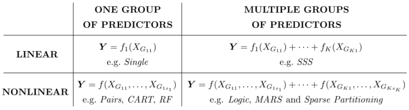
concern-ONE GROUP MULTIPLE GROUPS OF PREDICTORS OF PREDICTORS LINEAR Y =f1(XG11) e.g. Single Y =f1(XG11) +· · ·+fK(XGK1) e.g.SSS NONLINEAR Y =f(XG11, . . . , XG1s1)

e.g. Pairs, CART,RF

Y =f(XG11, . . . , XG1s1) +· · ·+f(XGK1, . . . , XGKsK)

e.g. Logic,MARS andSparse Partitioning

Figure 1.2: Classification of regression methods. I have categorised methods according to two fea-tures of their underlying relationships: whether they permit more than one group of predictors and whether they permit more than one predictor in each group. This table shows the four possibilities and lists some methods in each category. Single, Pairs and Sparse Partitioningare my own implementa-tions, while CART, RF, SSS, Logic and MARS refer to existing methods, all of which I describe in the main text.

ing the form of the true underlying relationship. In large p, small n problems, it is common

to apply a sparsity assumption, one which supposes that only a small number of predictors are causal. This assumption might seem debatable. In the context of association studies, it is in line with the common disease, common variant hypothesis, the validity of which has been questioned. Similarly, from speaking to members of the Nordborg Lab, who concentrate on

Arabidopsis thaliana, they are coming around to the idea that some traits may be affected by

many tens of causalities, many of which have only a tiny effect on the phenotype.

Fortunately, I feel that, in some sense, the validity of this sparsity assumption is irrelevant. If it is the case that vast numbers of causal predictors do influence a response, there is no hope of identifying them all for standard sample sizes, so an assumption of this nature is nec-essary. Perhaps more accurately, however, the assumption can be worded as a prior belief in the number of “strong associations”. Therefore, when I discuss “the search for associations”, this phase can be interchanged with “the search for strong associations”, depending on one’s point of view.

A regression method can be classed as linear or nonlinear, depending on whether or not it permits interactions between predictors. In terms of my expression for the underlying relation-ship, this very closely corresponds to whether the method allows only one, or more than one, predictor in each group. In a similar fashion, a method can be classified based on whether it permits only one, or more than one, group of predictors. This creates four possible categories,

as demonstrated in Figure 1.2.

(28)

cate-gorical predictors. There are areas, most notably that of functional data analysis, which are devoted to regression with quantitative predictors. Typically, these are designed for small

numbers of predictors, and their focus is on prediction (explicitly calculating f(X)), rather

than variable selection (identifying the groupings). Methods in this area often opt for spline

fitting, a topic I discuss more in Chapter6.

1.4.2 One Group, Maximum Group Size One

f(X) = f1(XG11)

The simplest assumption supposes that the underlying relationship, and therefore the response,

is influenced by only one predictor. If predictorg takes only two values, any non-trivial

func-tion ofXg will have two degrees of freedom and can be written as f1(Xig) =θ1Xig. If Xg takes

more than two values, it is necessary to decide whether to treat these values as categorical or quantitative. If categorical, the function is again a mapping of distinct points, taking the form

f1(Xig) = θ1d, wheredindicates to which image the stateXig is assigned. This can be written

as the linear model f1(Xg) = J1θ1, where the dth column of J1 indicates which samples are

mapped toθ1d. The most general form forf1(Xg) has degrees of freedom equal to the number

of distinct values for Xg. However, we can also consider forms with less degrees of freedom,

insisting that distinct predictor states are mapped to the same image: f1(Xig) =f1(Xi0_g) for

some Xig 6=Xi0_g.

If quantitative, the function can be viewed as a curve, whose domain includes the possible predictor values. In theory, there is no limit to the degrees of freedom of this curve; in practice,

when the degrees of freedom exceeds the number of unique values observed forXg, there will

be some redundancies. For genetic applications, it is very common to use the simplest

non-trivial curve, a straight line, in which case the model takes the form f1(Xig) = θ10+θ11Xig.

Here, the intercept termθ10represents the baseline value, while the gradientθ11 indicates how

much each unit change inXg affects the underlying relationship. Again, this is easily written

asf1(Xg) =J1θ1, by lettingJ1 = [1 Xg], where 1 is a vector of ones.

As there are only N choices for the causal predictor, it is straightforward to explore all

possibilities. Having decided on a functional form, most frequentist methods in this category are equivalent to performing a maximum likelihood test for each predictor, comparing the

null hypothesis, f(X) = constant, with the alternative, f(X) = f1(Xg). It is easy to create

a Bayesian counterpart (e.g. Balding, 2006), which instead calculates the Bayes factor or

posterior probabilities for the null and alternative hypotheses. Such a version is useful when we have prior knowledge of how likely it is that each predictor is associated.

(29)

its marginal effect. For example, when testing whether a binary predictorXg is associated, the

methods will compare the response values when Xg = 0 to those whenXg = 1. Discordance

between these two sets of values provides evidence thatXg has an effect on the response.

Nat-urally, these methods perform best when the true underlying relationship actually is affected by just one predictor. When this is not the case, the presence of additional causal predictors will generally diminish each association’s marginal effect and so these methods’ power to de-tect.

These methods have proven very popular for the analysis of association study data. This

owes much to their simplicity; they only requireN comparisons, so computation time is kept to

a minimum, and their conclusions can be explained to someone with only a basic understanding of statistics. Furthermore, considering how simple their underlying relationship assumptions, these methods have been surprisingly successful. In association studies, many hundreds of causal variants have been identified using these “one-predictor-at-a-time” approaches, some of

the most high-profile finds coming from_{The Wellcome Trust Case Control}

Consor-tium (2007, 2010). For these reasons, methods of this type typically form the starting point

for any analysis.

Single is my implementation of a method in this category, offering both a frequentist and

Bayesian analysis. For the latter, given a prior probability of association for each predictor, it

calculates a posterior probability of association. For the frequentist version, Single performs

a maximum likelihood test and returns a p-value. I explain this method in more detail in

Chapter 4, in particular showing the similarity between posterior probabilities and p-values

when a uniform prior is used.

1.4.3 One Group, Maximum Group Size Greater Than One

f(X) =f1(XG11, . . . , XG1s₁)

When s1 = 2, there are N₂

choices for the pair of interacting predictors and it will gen-erally remain feasible to test all possibilities. In the case of very high-dimensional problems, which might have upwards of 500,000 predictors, an implementation of such a search may take

many hundreds of computing hours (cf. Marchini et al., 2005), although this can be offset

with parallelisation.

When the predictors are categorical, the underlying relationship will assume the form

f1(Xig, Xig0) =θ_1d, where d indicates to which image the vector (X_ig, X_ig0) relates. The

num-ber of unique values of d determines the degrees of freedom, and therefore the flexibility, of

the model. Again, this is readily represented as a linear model, by constructing the matrix

(30)

are quantitative, there is no obvious choice for the functional form. One possibility might be f1(Xg, Xg0) = f₁₁(X_g) +f₁₂(X_g0) +f₁₃(X_g, X_g0), where f₁₁ and f₁₂ represent the additive

contributions of Xg and Xg0, while f₁₃ tries to capture the “interaction term”.

Pairs is my implementation of a method in this category. Designed for categorical

pre-dictors, it simply extends Single to additionally consider alternative models of the form

f1(Xig, Xig0) = θ_1d, with full degrees of freedom. For each possible alternative model, it returns

ap-value and posterior probability by comparing this to the null model f(X) = constant. It

is easy to imagine extending this method further, to exhaustively try all three or four-way interactions, but for all except the smallest problems, such a method would typically take far too long.

Classification and Regression Trees (CART; Breiman et al., 1984) is another method in

this category, one which can be applied to both categorical and quantitative predictors. CART

explores the space of decision trees, each of which defines a partitioning of the samples. Within a decision tree, each internal node divides a set of samples into two groups based on the value

at a specified predictor. For example, the samples with Xig ≤ 1 might be directed into one

group, those with Xig >1 into the other. Each decision tree is scored based on its ability to

explain the observed response values; a tree will score highly if its partitioning groups sam-ples with similar response values. Once again, each model can also be written in the form

f(X) =J1θ1. In this case, the dth column of J1 indicates which samples are assigned to the

dth group of the partition.

CART implements a forwards regression search. At each step, it decides whether to add a

predictor into the current model, which equates to adding a node to the current decision tree. As each additional predictor will generally improve the model fit, it is common to introduce a penalty term to control the model’s growth. An alternative is to let the search continue until no further improvement is possible, which might well result in a tree that assigns each sample to its own group and therefore has perfect fit. At this point, the tree can be “pruned” to the desired size by removing predictors, in a process known as “backwards regression”.

A noticeable difference betweenCART and Pairs is that the former does not insist on the

full interaction model for associated predictors. For example, suppose for binary predictors

CART decides to split the samples first based on whether Xg = 1, then splits the samples for

which Xg = 1 by their value at Xg0. This model will produce three groupings so have three

degrees of freedom, even though four unique vector values of (Xg, Xg0) might be present.

Random Forests (_Breiman, 2004) offers a stochastic interpretation ofCART. Out of then

(31)

iteration, a decision tree is constructed using n0 samples picked with replacement from the training set (“a bootstrap sample”). Each node of this decision tree is determined by choosing

N0 << N predictors at random from all those available, and selecting the one which provides the best improvement in fit. Nodes are added until no further improvement is possible. Having grown a number of trees in this way, each can be scored according to its prediction accuracy for the samples in the test set. Finally, an importance weighting is calculated for each predictor

by averaging the scores of all trees in which it appears. RF offers a practical implementation

ofCART for very large numbers of samples. The choice of N0 serves as the penalty term, and

can be interpreted as the prior belief in the correct number of associations. RF does not draw

conclusions based on a single best fitting model, but instead calculates a weighted average

over a number of models. The idea of model averaging, (discussed by Hoeting et al., 1999;

Wassserman, 2000, among others) is one which, as I will show later on, seems generally a

better strategy.

1.4.4 More Than One Group, Maximum Group Size One

f(X) =f1(XG11) +f2(XG21) +· · ·+fK(XGK1)

This underlying relationship allows more than one predictor to be causal, but insists that the causal predictors contribute independently and additively. When we introduce more than one function, it may be necessary to safeguard against unidentifiability. For example, if we have

two functions, each of the formfk(Xig) = θk0+θk1Xig, it is possible to alterθ10 and θ20

with-out changing f1 +f2. The easiest solution to this problem is to merge each θk0 into a global

intercept θ0. In this case, the degrees of freedom of the model reduces from 2K to 1 +K.

Similarly, if using functions of the form fk(Xig) = θkd, we can introduce a global intercept

term θ0, which acts as a base value, and assign θk1 = 0, for k = 1,2, . . . , K. Again, the total

degrees of freedom will be reduced by K−1.

For categorical predictors, each fk, and therefore P_kfk, can be represented by a linear

model. An all-inclusive approach is to let K = N and write the underlying relationship as

f(X) = JΘ, where J = [1 J1 J2· · ·JN] and Θ = [θ0,θ1,θ2, . . . ,θN]. In this model, θg

represents the coefficients specific to predictorg. In most cases, the degrees of freedom of this

function will far exceedn. Therefore, it becomes necessary to encourage mostθg to have either

zero (or negligible) magnitude, indicating that predictor g does not (significantly) contribute.

In the frequentist set-up, there are many flavours of penalty term which will have the desired effect. Perhaps the simplest of these is “variable subset selection”, which enforces a penalty based only on the number of non-zero regression coefficients. An example penalty

(32)

sum of squares by an amount proportional to the number of non-zero coefficients. Variable subset selection generally uses a stepwise search of the model space. Each model dictates which regression coefficients are non-zero, conditional on which the best fit can be calculated using the least squares estimates.

“Ridge regression” is a description given to methods which penalise based on the sum of

the squares of regression coefficients (e.g. Zhang and Xu, 2005; Park and Hastie, 2008).

By contrast, the LASSO method penalises according to the sum of their absolute values (

Tib-shirani, 1996). Generally, the penalty term is prefaced by a scale factor λ, so that as λ→0

the solution approaches the least squares estimates. Ridge regression and the LASSO can

be compared by considering their effect on the best fit as λ is increased from zero. For ridge

regression, the least squares estimates of the regression coefficients are reduced in a continuous

fashion, only reaching zero whenλ =∞. For the LASSO, the estimates reach zero at

differ-ent points, depending on the predictors’ relative contributions to f(X). This highlights the

differences between each method’s sparsity assumption. The former supposes that there are a few strong associations, while most predictors contribute only slightly; the latter supposes most predictors contribute in no way at all.

Many frequentist methods have Bayesian analogies. For example, variable subset selection

equates to placing a point mass on elements of Θ (e.g. _Kuo and _Mallick, 1998), ridge

re-gression corresponds to a normal prior (e.gZhang et al., 2005; Wanget al., 2005), while the

LASSO relates to a double-exponential distribution (e.g. Yi and Xu, 2008; Hoggart et al.,

2008).

The use of mixture priors allows more complicated methods to be devised. Shotgun

Stochastic Search (SSS; Hans et al., 2007) is one of these. Given a prior probability of

association p ∈ (0,1), it assigns the regression coefficient corresponding to the gth predictor

the spike and slab prior distribution

P(θg) = (1−p)δ{0}+pN(0, σ2),

whereδ{0} represents a point mass function at 0 which “integrates” to 1, andN(0, σ2) denotes

a normal distribution with mean 0 and varianceσ2. SSS searches the model space in a stepwise

fashion, at each step deciding whether to add in, swap out or remove a contributing predictor. The method calculates the posterior scores for all models within the “neighbourhood” of the current state; those models reachable by a single move of the type add, swap or remove. Based

upon these scores,SSS constructs a proposal distribution from which it picks which model to

(33)

SSS keeps track of the top scoring models it explores, from which it estimates posterior probabilities of association for each predictor. The accuracy of these estimates depends on the

extent that the model search succeeds in identifying the best models. In essence, SSS tries to

approximate the complete space of models by its list of top scoring models, so the greater the proportion of posterior weight contained within this list, the more accurate the approximation

will be. As_Hanset al. discuss, rather than at each step automatically accepting the proposed

move, they could instead adopt a conventional MCMC strategy and calculate an acceptance probability. The method could then calculate posterior estimates in the normal fashion, based on how often each predictor is included in the Markov Chain. The authors conclude, however, that their search is preferable.

For quantitative predictors, this category of underlying relationship takes the form of the

generalized additive model (_Hastieand_Tibshirani, 1990), with a Bayesian version discussed

in _Ravikumar (2009). As with functional data analysis, these methods are suited for very

small numbers of predictors and when prediction, rather than variable selection, is the main focus.

1.4.5 More Than One Group, Maximum Group Size Greater Than

One

f(X) =f1(XG11, . . . , XG1s₁) +f2(XG21, . . . , XG2s₂) +· · ·+fK(XGK1, . . . , XG_KsK)

Allowing both interactions and multiple groups of predictors to contribute to the underlying relationship has the potential of most accurately describing the true model. However, both decisions increase the size of the model space and so the difficulty of identifying this true model. Relatively speaking, a limited number of methods fall into this category.

Logic Regression (Logic) is one such method, suitable when the predictors are binary. Logic

creates new predictors, each of which are logical functions of the original ones. For example,

one new predictor might be XC

1 ∨(X2∧X3), where ∨and ∧ represent the Boolean functions

“OR” and “AND”, and XC

1 is the complement ofX1. This predictor takes value one if either

X1 is zero or both X2 and X3 are one. Logic then fits a linear model with these new

predic-tors. Each predictor is allowed to feature in more than one group, which allows the search of

a broader range of interactions. For example, while each of f1(X1, X2) = θ10+θ11X1∧X2 and

f2(X1, X2) =θ20+θ21X1C ∧X2C have 2 degrees of freedom, a linear combination of f1 and f2

remains a function of X1 and X2, but has degrees of freedom 3.

Logic operates in two flavours: it either explores the model space in a frequentist

(34)

Bayesian search, using MCMC to produce estimates of posterior probabilities of association

(Kooperberg and Ruczinski, 2005). If the predictors are tertiary, the method suggests

recoding each as two variables, whereby 0, 1 and 2 are transformed to (0,0), (1,0) and (1,1),

respectively. In genetic terms, the two new predictors represent the dominant and recessive

components of the original variant. To apply Logic to quantitative predictors, it would be

necessary to recode each predictor as one or more binary variables, for example, thresholding

values in a manner similar to CART.

Multivariate Adaptive Regression Splines (Friedman, 1991) is a second method in this

category, primarily designed for continuous predictors. MARS also places restrictions on the

types of functions permitted, considering only products of hinge functions:

fk= Θk

Y

j

h(Ggj, iGgj),

where either h(g, i) = max(0, Xg −Xig) or h(g, i) = max(0, Xig −Xg). Each h(g, i) is only

non-negative on one side of its corresponding knot Xig. Therefore, the product of functions

of this type will be non-negative over an ever-decreasing proportion of the input space. As

a result, MARS is able to model changes over very fine scales, allowing it to pick out local

variation. _Denison and _Holmes (2003) consider a Bayesian version of this method.

Sparse Partitioning, the method to which I devote the remainder of this thesis, falls into

this category, but unlikeLogic andMARS it attempts to apply no restrictions to the functions.

1.4.6 Other Methods

So far, I have focused on regression methods which can be applied when the response is con-tinuous. Partly, this is because a continuous response should provide more information than a binary one, a property which becomes increasingly important when considering interactions. Furthermore, any regression method suitable for continuous values can be either adapted for, or applied directly to, a binary response, whereas the converse is not true. Here, I mention methods for analysing binary response data, as well as one further method suitable for a con-tinuous response. Most of these methods loosely fall into the category “one group, maximum group size greater than one”.

Sparse combinatorial inference (Mukherjeeet al., 2009) considers the contingency table

formed by a single group of interacting predictors (K = 1; s1 = 1,2,3, . . .). For example, for

two binary predictors, the table will have four cells, counting the number of occurrences of

(0,0), (0,1), (1,0) and (1,1). To each cell, the method assigns a parameter, which represents

(35)

each contingency table is scored in a Bayesian fashion, according to how well it fits the data. The method seeks to deduce the most plausible grouping using MCMC.

The approach of multifactor dimensionality reduction (Hahnet al., 2002) is very similar,

but set within a frequentist framework. First, the method splits the samples into a training and test set. For a given contingency table, it assigns each cell value either 1 (“high risk”) or

0 (“low risk”) according to the numbers of cases (Yi = 1) and controls (Yi = 0) in the training

set to which this cell corresponds. The table is then scored by using these assignments for the test dataset, counting how many of the response values it correctly predicts. Rather than ex-plore the model space in a stepwise fashion, multifactor dimensionality reduction exhaustively scores each possible contingency table, returning the best one found. As a table’s prediction accuracy will depend on the choice of training and test sets, to obtain a reliable score it is necessary to repeat this procedure for a number of divides. The exhaustive nature of the search places a limit on the sizes of models and dataset the method can consider.

Verzilliet al.(2006) construct a Bayesian graphical model, one which considers the joint

likelihood of the response and the predictors. Designed for association study data, the method searches for the best division of predictors into cliques, where each clique indicates dependency between the variants it contains. Each graph defines three types of predictor. Those “directly” associated with the phenotype lie in a clique containing the response. Those “indirectly” as-sociated can be linked to the response via one or more other cliques. However, the majority of predictors occur in cliques completely disjoint from the response, indicating they are in no way associated. The graphical structure enables the method to account for LD, so hopefully allow-ing it to more accurately detect associations when strong correlations exist between predictors.

Mailund et al. (2006) also take a graph-based approach, devising a method which

in-corporates coalescent theory. For each locus, first they create the phylogenetic tree which explains that predictor and as many neighbours as possible. This tree will divide the samples according to the end branch on which each lies, so can be scored by comparing this partition-ing with the response. By regresspartition-ing on trees, rather than individual predictors, the method is able to consider LD and possible interactions over the (local) area on which the tree is defined.

BAMSE (Bayesian Association for Multiple SNP Effects; Albrechtsen et al., 2007) is

predominantly designed for a continuous response. The method considers multiple groups of associated predictors, each of which defines a “risk set” of samples and is assigned a mean

phe-notypic value. For example, one risk set might contain all samples with X1 >1 and X2 <2,

while a second might include all samples with X3 > 0. Although BAMSE allows multiple

groups of associations, under my terminology it falls into the category “one group, maximum group size greater than one”; when a sample satisfies the conditions for two or more risk sets,

(36)

it is assigned only to the one with the highest phenotypic mean. Therefore, just likeCART, each model dictates a partitioning of the samples, and can be described by a single design

matrix J1, with corresponding parameter vector θ1. The space of possible configurations of

risk sets is explored using MCMC.

Two final methods are Combinatorial Partitioning (_Nelson et al., 2001) and BEAM

(37)

Chapter 2 Sparse Partitioning

This chapter outlines the core of Sparse Partitioning’s methodology, saving superfluous details

for later. Sparse Partitioning is suitable only for problems with tertiary predictors, those that

can be represented by values from 0, 1 or 2. These predictors are treated as categorical, so their order and the choice of labelling is irrelevant.

2.1 Motivation

In the previous chapter, I expressed the underlying relationship as the sum of functions of groups of predictors:

f(X) =f1(XG11, . . . , XG1s₁) +f2(XG21, . . . , XG2s₁) +· · ·+fK(XGK1, . . . , XG_KsK),

with predictors free to feature in more than one group. Let’s suppose we are given the groups

of predictors and wish to explore possible sets of functions f ={f1, f2, . . . , fK}. How many

different forms are there for each fk, bearing in mind we are considering categorical

predic-tors? Let’s examine the simplest case, a function of two binary predictors fk(Xg, Xg0). In

total, there are up to four distinct values (nodes) for (Xg, Xg0), namely, (0,0), (0,1), (1,0) and

(1,1). Each suitable function provides a mapping of each node to a real value: fk:{0,1}2 7→R.

The function need not permit different nodes to map to different values. Instead, it

may insist, say, that fk(0,0) = fk(0,1). The degrees of freedom of the function is equal

to the number of free parameters. This will equal 4 if all nodes are allowed to map to

different values, less than 4 if there are restrictions. Figure 2.1 displays the different

func-tional forms possible for degrees of freedom 2, 3 and 4 (the case when the degrees of

free-dom equals 1 is ignored, as then the function would be trivial). In total, there are 14

possible forms, however, two of the forms with degrees of freedom 2 are disallowed: when

Exploring nonlinear regression methods, with application to association studies