Biomedical Applications
Bingzhi Zhang
Submitted in partial fulfilment of the requirements for the degree
of Doctor of Philosophy
in the Graduate School of Arts and Sciences
COLUMBIA UNIVERSITY
Bingzhi Zhang All Rights Reserved
On Compositional Data Modeling and Its
Biomedical Applications
Bingzhi Zhang
Compositional data occur naturally in biomedical studies which investigate changes in the proportions of various components of a combined medical measurement. The statistical method to analyze this type of data is underdeveloped. Currently the multivariate logit-normal model seems to be the only model routinely used in analyzing compositional data, and its application is mainly in geology and has yet to be known to the biomedical fields. In this dissertation, we propose the multivariate simplex model as an alternative method of modeling compositional data, either cross-sectional or longitudinal and develop statistical methods to analyze such data. We suggest three approaches to making a fair comparison between the multivariate simplex models and the multivariate logit-normal models. The simulations indicate that our proposed multivariate simplex models often outperform the multivariate logit-normal models.
1 Introduction and Motivating Examples 1
2 Proportional Data Modeling 10
2.1 Ad hoc methods for modeling proportional data . . . 10
2.2 Modeling proportional data using simplex distribution . . . 16
2.2.1 Simplex distribution . . . 16
2.2.2 Simplex GLM . . . 17
2.2.3 Comparison between the univariate simplex model and the logit-normal model . . . 20
2.2.4 GEE simplex GLM . . . 22
2.2.5 An illustration study . . . 24
3 Compositional Data Modeling 26 3.1 Existing methods . . . 26
3.1.1 Dirichlet distribution . . . 27
3.1.2 Multivariate logit-normal model . . . 27
3.2 Multivariate Simplex Model . . . 29
3.2.1 Multivariate simplex distribution . . . 29
3.2.2 Properties of the multivariate simplex distribution . . . 30
3.2.3 Score function . . . 32
3.2.4 Fisher’s information matrix . . . 33
3.2.5 Probability density function plots of 2-dimensional simplex distribution 34 3.2.6 Multivariate simplex GLM . . . 34
4.2 Compare multivariate simplex models with multivariate logit-normal models 39
4.2.1 Case I: multivariate simplex models are the true models . . . 39
4.2.2 Case II: multivariate logit-normal models are the true models . . . . 49
4.3 Multivariate simplex models with continuous, non-linear, and interaction pre-dictors . . . 57
4.4 Multivariate simplex models with more than 3 components . . . 59
5 Clustered Compositional Data Modeling 62 5.1 Multivariate simplex GEE models . . . 64
5.1.1 Model specification . . . 64
5.1.2 Parameter estimation . . . 65
5.2 Multivariate simplex mixed effects models . . . 67
5.3 Simulation studies . . . 69
5.3.1 Generating random vectors with arbitrarily specified marginal distri-butions and correlations: NORTA method . . . 70
5.3.2 Generating random vectors with multivariate simplex marginals and specified correlation matrix . . . 73
5.3.3 Simulation Study for multivariate simplex GEE models . . . 75
6 Applications to Real Data in Biomedical Research 78 6.1 Physical activity data . . . 78
6.1.1 Data description . . . 78
6.1.2 Data analysis . . . 82
6.2 Cascade impactor deposition profile data . . . 89
6.2.1 Data simulation . . . 90
6.2.2 Data analysis . . . 93
7 Future Works 97
Bibliography 100
1.1 Linear regression fit to body fat percentage data. . . 3
1.2 Histograms of reading accuracy by groups. . . 4
1.3 Residual plot of linear regression for reading accuracy data. . . 5
1.4 Structure of CI by stages. . . 9
2.1 Probability density function of beta distributions. . . 12
2.2 Probability density plot of simplex distribution . . . 18
3.1 Pdf plots of simplex distributionS2(µ, λ) . . . 35
4.1 Sediment components by water depth (in log scale) . . . 55
5.1 Mean curves for GEE and GLMM. . . 64
5.2 MLP with one hidden layer. . . 72
6.1 Mean CI depositions for reference products and test products . . . 91
1.1 Classification by body fat percentage . . . 2
1.2 Ranks of physical activities EE by subgroup . . . 7
2.1 OLS and Beta regression for reading accuracy scores . . . 13
2.2 Median regression for reading accuracy scores . . . 15
2.3 Comparison between univariate simplex GLM and logit-normal model . . . . 21
4.1 Comparisons on parameter estimation when data are multivariate simplex distributed . . . 41
4.2 Comparing the estimated MSE when data are multivariate simplex distributed 43 4.3 Comparisons on powers and type I errors when data are multivariate simplex distributed (alternative: β= (0,−0.3,0,0.3)) . . . 44
4.4 Comparing TIC when data are multivariate simplex distributed . . . 49
4.5 Comparisons on parameter estimation when data are multivariate logit-normal distributed . . . 51
4.6 Approximated expectation of logit-normal distribution by numerical integra-tion and simulaintegra-tion . . . 52
4.7 Comparing the estimated MSE when data are multivariate logit-normal dis-tributed . . . 52
4.8 Comparing powers and type I error rates when data are multivariate logit-normal distributed . . . 53
4.9 Comparing the estimated TIC when data are multivariate logit-normal dis-tributed . . . 54
4.10 Multivariate simplex model with clay as reference component . . . 56
4.13 Parameter estimates by multivariate simplex model for compositional data
with 5 components . . . 60
4.14 Parameter estimates by multivariate simplex model with reduced dimension 61 5.1 Parameter Estimates by multivariate simplex GEE for clustered compositional data . . . 77
6.1 Top ten physical activities by percentage of energy expenditure . . . 80
6.2 Demographic characteristics of sample . . . 81
6.3 Multivariate simplex model with sleeping as the reference activity . . . 83
6.4 Multivariate simplex model using grooming as the reference activity . . . 84
6.5 Multivariate simplex model using eating as the reference activity . . . 85
6.6 Multivariate simplex model using cooking as the reference activity . . . 86
6.7 Multivariate simplex model with sleeping as the reference activity . . . 89
6.8 Mean CI depositions for reference products and test products . . . 91
6.9 Standard deviations ofR0ij and Tij0 , . . . 92
6.10 Correlation R . . . 92
6.11 Parameter estimates and p-values for testing componentwise effect . . . 94
I would like to express my deepest gratitude to my advisor, Dr. Bin Cheng. I am very fortunate to have him as a great mentor and supporting friend. His patient instruction and encouragement have helped me overcome difficulties and build confidence. I am constantly amazed by his breadth and depth of knowledge and wisdom in life. The countless discussions with him are and will always be a great treasure for me. Without him, my dissertation would be impossible and my graduate experience would be much less rewarding. I hope I could become someone like him who continuously enlightens others by his knowledge and ideas with great generosity.
I am very grateful to Dr. Wei-Yann Tsai, Dr. Srikesh Arunajadai, Dr. Gina Lovasi and Dr. Shuang Wang for serving as my dissertation committee members. I am thankful to the Biostatistics Department and the Mailman School of Public Health at Columbia for thoughtfully designed courses and research opportunities. I am particularly thankful to Dr. Shuang Wang and Dr. Frederic P. Perera for the experience of working at Columbia Center for Children’s Environmental Health, and Dr. Myunghee Cho Paik who is my coursework advisor.
At last, I want to thank my parents Xiaoming Zhu and Hongming Zhang for their un-conditional love and support.
Chapter 1
Introduction and Motivating
Examples
Proportional data are continuous data taking values between 0 and 1. Such type of data arises naturally as estimated proportion of a binomial distribution. The statistical analysis of proportional data thus obtained is usually through logistic regression models. However, not all proportional data are associated with binomial distribution. For example, body fat percentage, an important outcome variable in obesity study, is the percentage of fat weight with respect to the total body weight in a person. A multivariate counterpart of the proportional data is the so calledcompositional data, consisting of vectors of proportions that sum to 1. In spite of the frequent occurrence of these types of data, the statistical methods to analyze them are ramified and there is no systematic method for routine use. The choice between competing methods are largely determined by convention and convenience. In this dissertation, we propose new statistical methods for modeling compositional data and discuss their uses in the biomedical field.
To motivate our research, we consider four examples as illustrations.
Example 1. Body fat percentage. Obesity has reached epidemic proportions globally, with more than 1 billion adults overweight at least 300 million of them clinically obese
-and is a major contributor to the global burden of chronic disease, including type 2 diabetes, cardiovascular disease, hypertension and stroke, and certain forms of cancer. The most widely used diagnostic tool to identify weight problems within a population is the body mass index (BMI), or Quetelet index. It is a statistical measure of body weight based on a person’s weight and height: BMI = mass(kg)/height(m2). Despite of its ease of measurement and calculation, the usage of BMI is controversial. It was originally designed to classify physically inactive individuals with an average body composition. Muscular people are often misclassified as overweight due to the BMI’s incapability of differentiating lean mass and fat mass. From the physiological point of view, it is not the degree of excess weight (as is measured by the BMI), but the degree of body fatness that is important as a risk factor of a spectrum of diseases (Deurenberg et al, 1998). So the studies used the BMI as outcomes were actually using a proxy of the measure of excess body fat.
A direct way to measure the body fat is often expressed as “Body Fat Percentage” or “Body Fat Percent.” It is the total weight of the person’s fat divided by the person’s weight and consists of essential body fat and storage body fat. The body fat percentage can be measured by techniques like near-infrared interactance, dual energy X-ray absorptiometry (DXA), and in vivo neutron activation. One of the common classification by body fat percentage is shown in Table 1.1:
Table 1.1: Classification by body fat percentage Classification Women (%fat) Men (%fat)
Essential fat 10-13% 2-5% Athletes 14-20% 6-13%
Fitness 21-24% 14-17% Average 25-31% 18-24%
The relationship between body fat percentage and BMI has been studied. The prediction equation for the total Caucasian population was given by Deurenberg et al (1998) as
Percent body fat (%BF) = 1.284 BMI + 0.20 Age−8.0,
which was obtained using linear regression and the fitted regression line is shown in Figure 1.1.
Figure 1.1: Linear regression fit to body fat percentage data.
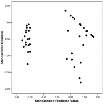
Example 2. Reading accuracy. In the previous example, data are scattered quite randomly along the predicted line, so the linear regression method is appropriate for the fat percentage data. However, this is not a universal truth for proportional data. Un-correctable skewness, heteroscedasticity, and multimodality of the dependent variable are common for data in biomedical research. An example was provided in the paper of Smithson and Verkuilen (2006). The data were supplied by K. Pammer in the School of Psychology at The Australian National University (Pammer & Kevan, 2004). The scores of the reading accuracy, dyslexic status and non-verbal IQ were collected on 44 children. The accuracy scores have been transformed to the interval [0,1] by taking y0 = yb−−aa, where b is the upper bound of the score and ais the lower bound. And theny0 is compressed to the open interval
(0,1) by y00 = [y0(n−1) + 1/2]/n, where n is the sample size. Applying the simple linear regression of the transformed accuracy scores on IQ and dyslexic status can lead to mislead-ing results. Histogram for the scores of the dyslexics and controls are in Figure 1.2. The
Figure 1.2: Histograms of reading accuracy by groups.
accuracy scores are highly skewed among the controls. And the residuals from the linear re-gression (Figure 1.3) indicate violation of the normality assumption. There is heterogeneity of variance between the two groups as well.
Example 3. Energy expenditure. The primary focus of researches and recommen-dations regarding physical activity used to be on sustained vigorous exercise. Such activity is usually obtained through purposeful, programmed behaviors, such as jogging, swimming, or sports participation. With these characteristics, vigorous exercise is relatively easy for respondents to report. Recent physical activity guidelines have emphasized the accumulation of shorter episodes of moderate intensity physical activity. Moderate-intensity activity can occur in many routine daily activities. Interventions to increase physical activity obtained through moderate-intensity daily activities have achieved comparable physiologic outcomes to those that used more vigorous programmed activities. However, monitoring behavior to assess moderate-intensity activities is a challenge because of the need to assess many
activi-Figure 1.3: Residual plot of linear regression for reading accuracy data.
ties of short duration that may occur as part of routine daily functions in varying contexts, e.g., transportation, occupation, household chores, as well as recreation and sport. Refer-ence periods for physical activity behaviors can vary from a week to a lifetime, and may focus on recent behavior, a specific previous period, or may be recorded contemporaneously. Ideally, physical activity assessment includes type of activity and context (specified by ques-tion content or respondent), frequency of behavior, duraques-tion of behavior, and performance intensity. Research pertinent to the assessment of physical activity has lagged behind. In particular, methods to evaluate measurement errors and algorithms to compensate for such errors through the use of statistical models and analytic procedures remain underdeveloped. Physical activities are linked to risk of chronic disease, such as coronary heart disease, non-insulin-dependent diabetes mellitus, and several types of cancer through mounting evi-dence (Pate et al. 1995). And it is found that the total energy expenditure (EE) is associated with gender, age, and ethnicity/race (Britton et al. 2002). For example, men expended sig-nificantly more energy per day than women and the 50 to 64 year olds had lower median EE
than those in the youngest group. However, not only the total EE is of interests, but also the composition of EE is worth investigation. For example the joint consideration of different aspects (e.g., bone-loading versus aerobic exercise) and sources of EE could be examined in relation to cancer outcomes. The contribution of a particular activity’s EE to the popula-tion’s EE can be expressed as the percent of overall population daily EE it accounted for. Here is an example of percent expenditure as part of table of physical activities accounting for 95% of the population daily energy expenditure among 373 participants, New York City, 1999-2000 (from Britton et al., 2002).
Table 1.2: Ranks of physical activities EE by subgroup
rank
Physical activity % of population EE population male Female Puerto Rican Black
Sleeping 18.9 1 1 1 1 1
Sitting quietly 7.46 2 2 2 2 3
Cooking 5.09 3 6 3 4 2
Eating 4.61 4 4 6 5 5
We can see that the rank of percent energy expenditure varies across subgroups by sex and race/ethnicity, which indicates that the demographic characteristics are non-uniformly associated with the various activity domains. Modeling the composition of EE based on the demographic variables and thus link these potential predictors to the related chronic disease outcomes could enable us to better identify the population of high risk and clarify the causal pathway.
Example 4. Nasal aerosol particle size distribution profile. The product quality bioavailability (BA) and bioequivalence (BE) of new drug applications (NDAs) or abbrevi-ated new drug applications (ANDAs) for locally acting drugs in nasal aerosols (metered-dose
inhalers(MDIs)) and nasal sprays (metered-dose spray pumps) are reflective of potency, in that release of the drug substance from drug product and the delivery to the mucosa should be assessed and controlled. BA and BE assessments for locally acting nasal aerosols and sprays are complicated because delivery to the sites of action does not occur primarily after systemic absorption. The topical deposition of droplets and/or drug particles which are absorbed through the nasal mucosa are the main source of local action. So from a product quality perspective, the critical issues are release of drug substance from drug product and delivery to the mucosa. Other factors are of less importance. In the guidance for BA and BE studies for nasal aerosols and nasal sprays for local action released by the United States Food and Drug Administration (FDA, 1999), the recommended approach for solution formulations is to rely on in vitro methods to assess BA and BE.
One of the tests which can characterize in vitro BA and BE for locally acting drugs delivered by nasal aerosol or nasal spray is Droplet and Drug Particle Size Distribution (PSD). To increase nasal deposition and minimize deposition in the lungs and gastrointestinal tract, aerosol droplets should generally have a mass median aerodynamic diameter (MMAD) greater than 10 to 20 microns. As MMAD decreases over the 5-20 micron range, the Task Group Report indicates that reduced nasopharyngeal deposition and increased pulmonary deposition occur. So droplet size distribution measurements are critical to the delivery of drug to nose, and it can be done by multi-stage cascade impactor (CI) based on inertial impaction, an important factor in the deposition of drug in the nasal passage.
Particles entering a CI pass through a plate containing one or more jets of well-defined size. A collection surface located immediately beyond the plate at a well defined separation distance deflects the flow; the inertia of the particles causes them to cross the flow stream, with the result that those with a size greater than a critical value impact on the surface, whereas smaller particles remain airborne. Several stages are arranged in sequence in a CI, such that particles having progressively finer sizes are collected as the aerosol passes through
the instrument (Mitchell et al, 2007). See Figure 1.4 for an illustration of a CI. Suppose there
Figure 1.4: Structure of CI by stages.
are S stages in the CI. LetXs be the deposition in mass unit at stages, wheres= 1,· · ·, S.
Then data can be expressed as S-dimensional vector X = (X1, . . . , Xs). A characterization
of particle/droplet size distribution is required for nasal aerosols. And one possible measure recommended by FDA is P = (p1, . . . , pS), where ps =Xs/PSi=1Xi. Let
PT = (pT1, . . . , pTS) and PR = (pR1, . . . , pRS)
be the profiles of a test product and a reference product, respectively. The profile difference between test and reference products is assessed by the following chi-square type measure
d(T, R) = S X s=1 (pTs −pRs) 2 (pTs +pRs)/2 ,
BE measure is suggested by FDA as RD=E " d(T,R+2R0) d(R, R0) # .
The profile BE is established if the following hypothesis is rejected at the 5% significance level
H0 :RD > θBE.
Note that profiles P’s are compositional data whose components might be correlated in a complicated way.
Chapter 2
Proportional Data Modeling
2.1
Ad hoc methods for modeling proportional data
This section provides a collection of the ad hoc statistical methods typically used in analyzing proportional data in medical fields.
One convenient method to analyze proportional data is by the arc-sine transformationλ= arcsin√p. It is noted that this transformation is appropriate for the proportions obtained from binomial distribution since the transformation produces normal distribution if the count follows a binomial distribution. Suppose X follows a binomial distribution Bin(n, p), then ˆ
p=X/n is the estimated proportion. By the central limit theorem, √n(ˆp−p) converges to N(0, p(1−p)) in distribution. The asymptotic variancep(1−p) is a function of the meanp. The arc-sine transformation is a variance stabilizing transformation. The sequence√n(ˆλ−λ) converges to a standard normal distribution for every p. However, for the percentage data such as % protein or % carbohydrates, which is not derived from the counts, the role of the arc-sine transformation is unjustified.
distribution. Ferrari et al. (2004) proposed a regression model where the response is assumed to be beta distributed. It is useful for situations where the variable of interest is continuous and restricted to the interval (0,1) and is related to other variables through a regression structure. The variableY follows a beta distribution if it has the probability density function
f(y|µ, φ) = Γ(φ)
Γ(µφ)Γ((1−µ)φ)y
µφ−1
(1−y)(1−µ)φ−1, 0< y <1,
where 0< µ <1 and φ >0. Since E(Y) =µ and Var(Y) =µ(1−µ)/(1 +φ), the variance is a function of µand the precision parameter φ. The regression model is specified as
g(µ) =
k
X
i=1
xTi βi
where g(.) is a link function that maps (0,1) into R1 and x
i’s are the covariates. Some
possible choices of the link function are the logit link g(µ) = log{µ/(1−µ)}, the probit link g(µ) = Φ−1(µ), where Φ is the cumulative distribution function (cdf) of the standard normal
random variable, and the complementary log-log linkg(µ) = log{−log{1−µ}}. Parameter estimations are performed by maximum likelihood estimation (MLE) method. Under the usual regularity conditions, the MLE estimates ( ˆβ,φ) are consistent and asymptoticallyˆ normally distributed. And the asymptotic inference can be performed using likelihood ratio, score, or Wald test.
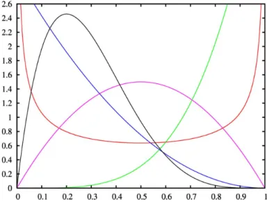
The above described beta regression is very similar to the generalized linear models (McCullagh & Nelder, 1989), except that the parameters β and φ are not orthogonal. The beta distribution is quite flexible as shown in Figure 2.1.
Instead of performing transformation on the data to stabilize the variance before linear regression, the beta regression model accommodates the heterogeneity of variance naturally because the variance of response is a function of the mean: Var(Y) = µ(1−µ)/(1 +φ), and it also allows for a precision parameter φ. Another advantage of this model is that when the logit link is used, the regression parameters can be interpreted in terms of odds ratio.
Figure 2.1: Probability density function of beta distributions.
The beta regression method is further generalized by Smithson and Verkuilen (2006) in the perspective that not only the mean, but also the precision parameter φ is modeled through h(φi) = wTi δ, where h is another link function. Since the precision parameter φ
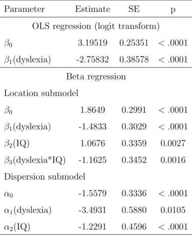
must be positive, the log link is an appropriate choice. MLE method is adopted to estimate δ. The reading accuracy scores can be re-analyzed by the beta regression model with logit link for the location submodel and log link for the dispersion submodel
logit(µ) = β0+β1 D +β2 IQ +β3 D×IQ, log(φ) = α0+α1D +α2 IQ,
where D = 1 for dyslexics, D = 0 for controls, and IQ is thez-score converted from nonverbal IQ. The coefficients, standard errors and significance tests are summarized in Table 2.1.
Table 2.1: OLS and Beta regression for reading accuracy scores Parameter Estimate SE p
OLS regression (logit transform)
β0 3.19519 0.25351 < .0001 β1(dyslexia) -2.75832 0.38578 < .0001 Beta regression Location submodel β0 1.8649 0.2991 < .0001 β1(dyslexia) -1.4833 0.3029 < .0001 β2(IQ) 1.0676 0.3359 0.0027 β3(dyslexia*IQ) -1.1625 0.3452 0.0016 Dispersion submodel α0 -1.5579 0.3336 < .0001 α1(dyslexia) -3.4931 0.5880 0.0105 α2(IQ) -1.2291 0.4596 < .0001
Unlike the OLS model, in the beta regression model IQ score has an independent contri-bution to the reading accuracy. And the significant interaction effect indicates that the posi-tive relationship between IQ and accuracy holds for the nondyslexic group ( ˆβ2 = 1.0676, p=
0.0027) but not for the dyslexic group ( ˆβ2+ ˆβ3 =−0.0949, p= 0.0669), which makes clinical
sense. Dyslexic readers have difficulty reading regardless of their general cognitive ability, whereas cognitive ability predicts reading accuracy for nondyslexics. Moreover, the standard errors in the OLS model are inflated because of its inability to account for the heteroscedas-ticity.
Assumptions on the distribution where the percentages are sampled can be relaxed by using non-parametric methods. One possible non-parametric test that we could adopt for
the proportions is the Wilcoxon rank-sum test. Suppose that we have two sets of proportions sampled from two groups, (p1, . . . , pn1) and (q1, . . . , qn2). And the null hypothesis is that the
distributions of both groups are the same. To get the test statistic, we first arrange all the observations into a single ranked series, and then add up the ranks for the observations which come from the same sample. Denote by R1 and R2 the rank sums of sample 1 and sample 2
respectively. The test statistic is given by either U1 =R1−
n1(n1+ 1)
2 orU2 =R2−
n2(n2+ 1)
2 .
For large samples, U1 (or U2) is asymptotically normally distributed with zero mean.
Non-parametric inferential method makes no assumption about the probability distribution, thus it is more robust to the parametric or semi-parametric methods. However, in cases where a parametric test would be appropriate, non-parametric tests have less power.
The Wilcoxon rank-sum test has another drawback that it can only deals with binary covariates or dichotomized covariates. When it comes to cases of continuous covariates, like the reading accuracy example, we must employ other non-parametric methods like quantile regression. Unlike OLS or GLM, which models the means of the variables of interests, quan-tile regression models the quanquan-tiles of the underlying distributions. Quanquan-tile regression is especially useful with data that are heterogeneous in the sense that the tails and the central location of the conditional distributions vary differently with the covariates. It provides a complete picture of the covariate effect when a set of percentiles is modeled, and so it offers the ability to capture important features of the data that might be missed by models that average over the conditional distribution. Because it makes fewer distributional assumption about the error term in the model beyond the mean 0 constraint, quantile regression offers considerable model robustness. It also offers a degree of data robustness. Unlike OLS regres-sion, it is robust to extreme points in the response direction (outliers). Median regression is an special case for the quantile regression which models the median of the dependent variable Y. For a random sample y1, . . . , yn, it is well known that the sample median minimizes the
sum of absolute deviations median = argminξ∈R
Pn
i=1|yi−ξ|. Median regression estimates
the linear conditional quantile function by solving ˆ β= argminβ∈Rp n X i=1 |yi−xTi β|.
Under mild conditions (Koenker and Bassett, 1982),
√
n( ˆβ−β)→Np(0, ω2(F)Ω−1),
whereω2(F) = 1/f2(F−1(1/2)) and Ω = limn→∞n−1PxixTi . Below we fit a median
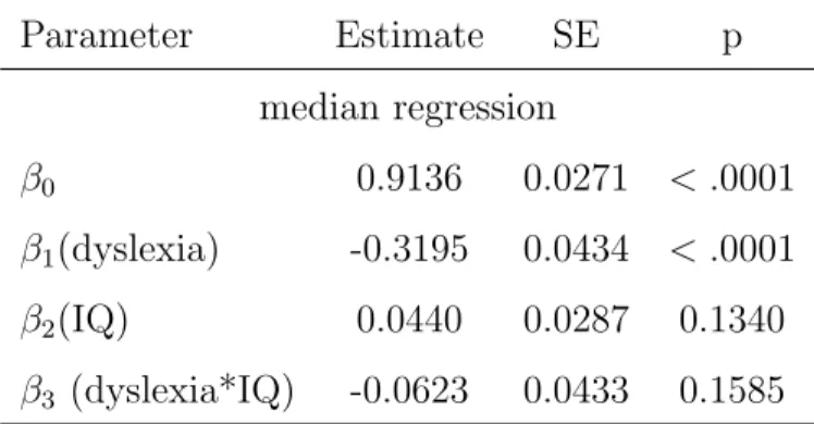
regres-sion using the previous reading scores as responses, dyslexia status, IQ z-scores and their interaction terms as predictors.
y=β0+β1 D +β2 IQ +β3 D×IQ +ε,
where is a median 0 random variable. The coefficients, standard errors and significance tests are summarized in Table 2.2. The significance of IQ and dyslexia-IQ interaction were lost in this median regression analysis, implying that the method might not be statistically efficient.
Table 2.2: Median regression for reading accuracy scores Parameter Estimate SE p median regression β0 0.9136 0.0271 < .0001 β1(dyslexia) -0.3195 0.0434 < .0001 β2(IQ) 0.0440 0.0287 0.1340 β3 (dyslexia*IQ) -0.0623 0.0433 0.1585
2.2
Modeling proportional data using simplex
distri-bution
2.2.1
Simplex distribution
The univariate simplex distribution, introduced by Barndorff-Nielsen and Jørgensen (1991), is a distribution suitable for modeling proportions. It is a special case of theproper dispersion model defined by Jørgensen (1987) as a family of distribution whose probability density functions is
f(y|µ, σ2) = a(σ2)v−12(y) exp
− 1
2σ2d(y;µ)
, (2.2.1)
where µ is the position parameter and σ2 the dispersion parameter, a is a suitable positive function, d is a regular unit deviancesatisfying
d(y;y) = 0 ∀y ∈Ω, (2.2.2)
d(y;y0)>0 ∀y 6=y0 and (2.2.3) ∂2d
∂µ2(µ, µ)>0 ∀µ∈Ω, (2.2.4)
and theunit variance function v of the regular unit devianced is defined as v(µ) = 2
∂2d
∂µ2(µ, µ). (2.2.5)
As a special case of the proper dispersion model, thesimplex distribution S(µ, σ2) with mean
µ∈(0,1) and dispersion parameter σ2 >0 has pdf
f(y|µ, σ2) = {2πσ2[y(1−y)]3}−1/2exp
− 1 2σ2d(y;µ) , (2.2.6) for 0< y <1, where d(y;µ) = (y−µ) 2 y(1−y)µ2(1−µ)2 (2.2.7)
is the unit deviance and v(µ) = µ3(1−µ)3 is the corresponding unit variance function. And the variance of y is provided by Jørgensen (1997) as
µ(1−µ)− √1 2σexp 1 σ2µ2(1−µ)2 Γ 1 2, 1 2σ2µ2(1−µ)2 , where Γ (s, t) is an incomplete gamma function defined by Γ(s, t) = R∞
s x
t−1e−xdx. Figure
2.2 shows the changing patterns of distribution density functions as µ and σ vary. The parameters µand σ have clear interpretations as position and dispersion parameter respec-tively. And also the family of simplex distribution covers a rich class of shapes from highly skewed to those very flat which implies that simplex distribution might be a suitable choice to model the proportional data which are usually skewed and multimodal.
2.2.2
Simplex GLM
Song (2007) utilized the simplex distribution to develop a generalized linear model for the proportional data by MLE. Let yi be the percentage response for theith subject and xi be
the corresponding p-dimensional vector of covariates, i = 1,· · · , n. Assume that yi follows
a simplex distribution with mean µi and dispersion parameter σ2, i.e., yi ∼ S(µi, σ2) and
µi depends on the covariates through the logit link, i.e., logit(µi) = xTi β, where β is a
p-dimensional vector of unknown parameters. The score equation for β is
n X i=1 xiµi(1−µi)ui =0, where ui =− 1 2 ∂d(yi, µi) ∂µi = yi−µi µi(1−µi) d(yi, µi) + 1 µ2 i(1−µi)2 .
Since the score function is not linear in yi by involving the nonlinear function d(yi, µi), it is
0.0 0.2 0.4 0.6 0.8 1.0 0 5 10 15 20 25 µ=0.1 σ 2 = 100 0.0 0.2 0.4 0.6 0.8 1.0 0 1 2 3 4 5 6 µ=0.5 0.0 0.2 0.4 0.6 0.8 1.0 0 5 10 15 20 25 µ=0.9 0.0 0.2 0.4 0.6 0.8 1.0 0 2 4 6 8 12 σ 2 = 20 0.0 0.2 0.4 0.6 0.8 1.0 0.0 0.5 1.0 1.5 0.0 0.2 0.4 0.6 0.8 1.0 0 2 4 6 8 12 0.0 0.2 0.4 0.6 0.8 1.0 0 2 4 6 8 σ 2 = 10 0.0 0.2 0.4 0.6 0.8 1.0 0.0 0.4 0.8 1.2 0.0 0.2 0.4 0.6 0.8 1.0 0 2 4 6 8 0.0 0.2 0.4 0.6 0.8 1.0 0 2 4 6 8 12 x σ 2 = 2 0.0 0.2 0.4 0.6 0.8 1.0 0.0 1.0 2.0 0.0 0.2 0.4 0.6 0.8 1.0 0 2 4 6 8 12 0.0 0.2 0.4 0.6 0.8 1.0 0 5 10 15 σ 2 = 1 0.0 0.2 0.4 0.6 0.8 1.0 0.0 1.0 2.0 3.0 0.0 0.2 0.4 0.6 0.8 1.0 0 5 10 15
requires the calculation of E12∂2(d(yi, µi))/∂2µi , where 1 2 ∂2d(y, µ) ∂2µ = 1 µ(1−µ)+ 1−2µ µ2(1−µ)2(y−µ) d(y;µ) + 1 µ3(1−µ)3 + 1−2µ µ4(1−µ)4(y−µ) − 1 µ(1−µ)(y−µ) ∂d(y, µ) ∂µ − 2(2µ−1) µ4(1−µ)4(y−µ).
To compute the expectation of the score function and Fisher information, we have to know E(d(y, µ)), E(y−µ)d(y;µ)) and E[(y−µ)∂d(y, µ)/∂µ]. The following propositions can be verified (see Song 2007).
Proposition 1. Let y ∼S(µ, σ2). Then,
1. E(d(y, µ)) = σ2;
2. E(y−µ)d(y, µ)) = 0;
3. E((y−µ)∂(d(y, µ))/∂µ) =−2σ2.
Using this proposition, we’ll have
E(ui) = 0, E 1 2 ∂2d(y, µ) ∂µ2 = 3σ 4 µi(1−µi) + σ 2 v(µi) . And the Fisher’s information for β is
I(β) = 1 σ2 n X i=1 1 + 3σ2µ2 i(1−µi)2 µ3 i(1−µi)3 xixTi ,
which is much simpler than its observed counterpart. Therefore, it is appealing to implement the Fisher scoring algorithm to get the MLE.
2.2.3
Comparison between the univariate simplex model and the
logit-normal model
Simplex GLM is computationally intensive. Alternatively, a linear model based on the logit-transformed data logit(yi) (the so called logit-normal model) seems theoretically and
computationally easier. It is of interest to compare the two models to see whether additional computational effort in fitting a univariate simple model is worthwhile. The parameters in a logit-normal model are usually more difficult to interpret. In addition, Song (2007) conducted a simulation study to compare the two models.
Specifically, Song (2007) considered the following univariate simplex model. Let yi, i=
1, . . . ,150,be independently generated from the simplex distributionS(µi, σ2), i= 1, . . . ,150,
where µi is linked to the covariates Ti and Si through
logit(µi) =β0+β1Ti+β2Si.
CovariateTi was randomly generated from a uniform distribution over{−1,0,1}andSi
ran-domly generated from a binomial distribution Bin(7,0.5). The true values of the parameters are set as β0 = 0.5, β1 = −0.5, β2 = 0.5 and σ2 = 400,200,50,0.5. For each combination,
200 data sets were generated and a simplex model and a logit-normal linear model were fit for each data set.
Song (2007) compared the two models in terms of estimation of β0s and their standard errors. Table 2.3 is a summary of the simulations results, including the averaged estimates, sample standard deviation of 200 replicated estimates and averaged estimated standard error based on Fisher’s information.
Table 2.3: Comparison between univariate simplex GLM and logit-normal model
Parameter Simplex model Logit-normal model
True mean sd se mean sd se
σ2 = 0.5 β0(0.5) .4996 .0280 .0254 .5089 .0288 .0263 β1(−0.5) -.5023 .0330 .0308 -.5110 .0345 .0322 β2(0.5) .5015 .0195 .0205 .5101 .0199 .0222 σ2 = 50 β0(0.5) .5062 .0983 .0960 .8057 .1769 .1752 β1(−0.5) -.5068 .1141 .1185 -.7998 .2065 .2148 β2(0.5) .5170 .0860 .0835 .8153 .1366 .1483 σ2 = 200 β0(0.5) .5060 .1145 .1021 1.0162 .2741 .2541 β1(−0.5) -.5262 .1346 .1263 -1.0479 .3218 .3114 β2(0.5) .5238 .0971 .0899 1.0430 .1919 .2150 σ2 = 400 β0(0.5) .5253 .0963 .1032 1.2306 .2767 .2980 β1(−0.5) -.5001 .1486 .1275 -1.1336 .3888 .3652 β2(0.5) .5165 .1000 .0909 .1.1686 .2286 .2521
Based on the above table, Song (2007) concluded that when the data are from a simplex distribution and the dispersion parameter σ2 is large, the performance of the logit-normal model may be questionable in the sense that its estimation is biased and not as efficient as the simplex model. Song (2007) also indicated that when data are simulated from a normal model, the univariate simplex analysis performs nearly as well as the logit-normal linear model, and when data are beta-distributed, the simplex model outperforms the logit-normal linear model.
2.2.4
GEE simplex GLM
Song and Tan (2000) utilized the simplex distribution to model longitudinal proportional responses. Let yij be the proportion response for the ith subject at time j and xij be the
corresponding p-dimensional vector of covariates, j = 1, . . . , ni, i = 1, . . . , K. Assume that
yij follows simplex distribution S(µij, σ2) and µij depends on the covariates through the
logit link logit(µij) =xTijβ, whereβ is the p-dimensional vector of parameters. Define ui =
(ui1,· · · , uini)
T, where u
ij =−12∂d(yij, µij)/∂µij. The Cowder optimality theory (Theorem
3.10 of Song, 2007) implies that the optimal equation in the sense of minimizing estimates’ errors is given by Ψopt(β,α) = K X i=1 DTi Ai[Var(wi)]−1wi =0, where wi = µ3i1(1−µi1)3ui1, . . . , µ3ini(1−µini) 3u ini
is the modified score residual vector, Ai = σ−2diag{v(µij)var(uij)} and DTi = ∂µTi /∂β. Since the variance-covariance matrix
Var(wi) is unknown and longitudinal or clustered observations are likely to be correlated,
Liang and Zeger (1986) suggested replacing the Var(wi) with a working covariance matrix
defined by
where Var(wij) = σ2µ3ij(1−µij)3{1 + 3σ2µ2ij(1− µij)2} and R(α) is an ni ×ni working
correlation matrix indexed by a q dimensional vector of parameters α. The estimating equation is Ψ1(β,α) = K X i=1 DTi AiV−i 1wi =0, (2.2.8)
The dispersion parameter σ2 is consistently estimated by ˆ σ2 = 1 PK i=1ni−p K X i=1 ni X j=1 d(yij; ˆµij). (2.2.9)
The estimating equation for the correlation parameters α is formulated based on the standardized score residuals rij =
uij √
Var(uij)
. We can see that E(rij) = 0, var(rij) = 1, and
E(rijrij0) = corr(uij, uij0) = corr(wij, wij0). Letri = (ri1ri2, ri1ri3,· · · , ri1rin
i, ri2ri3,· · · , rini−1rini)
T,
ηi =E(ri) and Wi is a working covariance matrix, the estimating equation for α is
Ψ2(β,α) = K X i=1 ∂ηTi ∂αW −1 i (ri−ηi) = 0.
Thus, the joint generalized estimating equations for θ= (β,α) are
Ψ(β,α) = Ψ1(β,α) Ψ2(β,α) =0.
Following the standard theory of estimating equations, the estimator ˆθ = ( ˆβ,α) is consistentˆ and K1/2(ˆθ−θ) converges in distribution to a multivariate normal distribution with zero
mean and covariance matrix of the form limK→∞KJ−1(θ), where J(θ) is the Godambe information matrix J(θ) =STV−1S. The sensitivity matrixS is
EΨ0θ(θ) = diag(S1,S2), (2.2.10) with S1 =EΨ0β(θ) = − K X i=1 DTi AiV−i 1AiDi,
and S2 =EΨ0α(θ) = − K X i=1 ∂ηT i ∂α W−i 1 ∂ηi ∂αT , and the variability matrix is
V =EΨ(θ)ΨT(θ).
2.2.5
An illustration study
Song and Tan (2000) gave an example of the application of above simplex GEE model and compared the result with the one based on logit-normal linear model. The longitudinal data used in the example arise from a prospective ophthalmology study, where gas was injected into the eye of 31 patients before surgery and the volume of the gas was recorded as a percentage of the initial gas volume in the eye at follow-up times after the surgery. It is important to estimate the decay rate of the gas over time and see how it is effected by the gas concentration.
First, a linear model was used to fit the logit-transformed responses logit(yij) on time tij
and gas concentration xij
log yij +a 1−yij +a =β0+β1tij +β2xij +eij,
whereais a small number added to avoid zero denominators. The AR(1) working correlation was used in the estimation. A normal-quantile plot of the residuals was used to check the normality assumption. It turned out that the shape of the plot varies significantly over varying values ofaand all these plots showed a S-shaped curve, which indicated the normality assumption is violated.
Song and Tan (2000) then directly model the response using the proposed simplex GEE model
The model was fitted assuming independent, exchangeable, and AR(1) working correlation structures, respectively. The estimates of the coefficients β’s did not differ much with differ-ent choices of working correlation. The quadratic time covariate log2(t) ws significant and dominated the linear term log(t), which matched the trend of the percentages over time. The estimated dispersion parameter was 14.2. The simplex distribution with such large dis-persion parameters has a dominant mass between 0.8 and 1, which is consistent with the fact that over 40% of the responses are in that range.
Chapter 3
Compositional Data Modeling
3.1
Existing methods
Compositional data is a collection of vectors u in the (m−1)-dimensional positive simplex
∇m−1 ={u∈Rm−1 :u
1+· · ·+um−1 <1, ui >0, i= 1, . . . , m−1}.
The analysis of compositional data is originally motivated by data from geological studies. For example, the compositions in terms of sand, silt, and clay percentages of 39 sediment samples at different water depths in an Arctic lake were given by Coakley and Rust (1968). Typical entries of the sedimentation data are
Sediment composition in percentage Water depth (meter) sand silt Clay
77.5 19.5 3.0 10.4
53.4 36.8 9.8 18.7
18.4 50.7 30.9 37.8
10.5 55.4 34.1 49.4
The question of interest here is how the compositional pattern depends on the water depth.
3.1.1
Dirichlet distribution
The Dirichlet distribution, a multivariate generalization of the beta distribution, is defined on the positive simplex and could be used to model compositional data. An (m−1)-dimensional random vector u= (u1,· · · , um−1)∈ ∇m−1 follows a Dirichlet distribution of order m−1 if
it has probability density function
f(u|α) = m Y i=1 uαi−1 i /B(α), where um = 1−Pm −1
i=1 ui, α = (α1,· · · , αm), and B(α) is the multinomial beta function
which can be expressed in terms of the gamma function asB(α) =Qm
i=1Γ(αi)
Γ(Pm
i=1αi).
There are drawbacks using Dirichlet distribution to model compositional data. First, the class of Dirichlet distributions is not rich enough to describe all patterns of correlations be-tween the composition components. For example, the pairwise covariance of the components is of the form cov(ui, uj) = −αiαj/(α2s(αs+ 1)) for i6=j, where αs=Pmi=1αi. This implies
that all the components of a Dirichlet distribution are pairwisely negatively correlated which may not hold for any compositional data. This suggests that the Dirichlet distribution may be too simplistic and restrictive to model general compositional data.
3.1.2
Multivariate logit-normal model
Aitchison and Shen (1980) proposed to model compositional data u by the following logit transformations from ∇m−1 toRm−1
The composition u follows a logit-normal distribution, denoted asLm−1(µ,Σ), if v follows
a multivariate normal distributionNm−1(µ,Σ). The probability density function ofu is
|2πΣ|−12 m Y j=1 uj !−1 exp −1 2(log(u/um)−µ) TΣ−1(log(u/u m)−µ) , u∈ ∇m−1.
The logit-normal distribution enjoys some good properties similar to the multivariate normal distribution. If v is Nm−1(µ,Σ) and B is a c×(m−1) matrix with entries {bij},
then Bv is Nc(Bµ,BΣBT). The corresponding transformation of u following Lm−1(µ,Σ)
is ti = m−1 Y j=1 (uj/um)bij ( 1 + c X i=1 d Y j=1 (uj/um)bij )−1 , i= 1, . . . , c.
That is,t = (t1,· · · , tc) is distributed asLc(Bµ,BΣBT). Using this property and selecting
B = 1 0 . . . 0 0 . .. 0 0 −1 . . . bhh=−1 −1 . .. 0 . . . 0 1 (m−1)×(m−1) ,
we conclude that t = (u1,· · · , th =um,· · · , tm =uh) follows an (m−1)-dimensional
logit-normal distribution with tm now the original uh. This means that the logit-normal form
is preserved no matter which (m−1) of the m positive quantities u1, . . . , um are chosen to
define the simplex of interests.
The logit-normal class Lm−1(µ,Σ) has 12(m−1)(m+ 2) parameters while the Dirichlet
class Dm−1 has onlym parameters. Aitchison (1982) claims that Lm−1(µ,Σ) is much richer
than Dm−1 and any Dirichlet distribution can be closely approximated by a suitable
logit-normal distribution, where the closeness of two distributions p and q is measured by the Kullback-Leibler distance defined as
DKL(p, q) = Z p(y)log p(y) q(y) dy.
In the rest of this section, we briefly present the maximum likelihood estimates un-der the multivariate logit-normal distribution. Let yi = (yi1, yi2, . . . , yim) with Pmk=1yik =
1, i = 1, . . . , n, be the compositional outcome and the logit-transformed outcome vi =
(log(yi1/yim),· · · ,log(yi,m−1/yim)) is linked to the covariates Xi via
vi =XTi β+εi
and εi follows multivariate normal distributionNm−1(0,Σ).
The maximum likelihood estimator of β is the least square estimator, and the MLE of
Σis ˆ Σ= 1 n n X i=1 (vi−XTi β)(vˆ i−XTi β)ˆ T.
3.2
Multivariate Simplex Model
Song’s work suggests that the univariate simplex distribution is flexible and efficient in mod-eling proportional data. It outperforms the logit-normal model when data are truly simplex distributed. For compositional data, as is seen in previous section, the model based on the multivariate logit-normal distribution has an edge over the model based on the Dirichlet distribution. These facts lead us to hypothesize that a multivariate version of the simplex dis-tribution might be a better model for compositional data than the multivariate logit-normal model.
3.2.1
Multivariate simplex distribution
Barndorff-Neilson and Jørgensen(1991) introduced the multivariate simplex distribution on the unit simplex ∇m−1 as the conditional distribution of m independent inverse Gaussian
inverse Gaussian distribution with pdf f(y|χ, ψ) = r χ 2πx3 exp −1 2 χx−1+ψx−2pχψ . (3.2.1) Let y1,· · · , ym be independent random variables such that yi is distributed as N−(χi, ψ).
Let y+ = y1 +· · ·+ ym. Then, y+ is again distributed as inverse Gaussian N−((
√
χ1 +
· · ·√χm)2, ψ). The multivariate simplex distribution, denoted as Sm−1(µ, λ), is the
condi-tional distribution ofy = (y1,· · · , ym) given y+ = 1, whose pdf is
λ 2π m2−1 m Y i=1 yi !−3/2 exp −λ m Y i=1 µi !−2/(m−1) m X i=1 (yi−µi)2/2yi , (3.2.2) where y= (y1,· · · , ym−1)∈ ∇m−1, ym = 1− Pm−1 i=1 yi, and µi = √ χi m X i=1 √ χi, i= 1,· · ·, m,
being the position parameter, and λ= m X i=1 √ χi !2 m Y i=1 µ 2 m−1 i
being the precision parameter. The parameter ψ disappears by conditioning due to the sufficiency for ψ of y+. Denote D(y,µ) = (
Qm
i=1µi)−2/(m−1)
Pm
i=1(yi−µi)2/yi, which is the
deviance function measuring the distance between the observation and its expectation. In the case of m = 2, the pdf (3.2.2) coincides the pdf of the univariate simplex distribution (2.2.6) with λ= 1/σ2 and D(y,µ) = d(y, µ).
3.2.2
Properties of the multivariate simplex distribution
In this section we present some properties of the multivariate simplex distribution to be useful in developing the proposed model and generating data in the simulation study.
Multivariate simplex distributionSm−1(µ, λ) consists of an exponential family with
canon-ical statistic (y1−1,· · ·, ym−1) by expressing (3.2.2) as
a(Θ) m Y i=1 yi !−23 exp ( m X i=1 θi yi ) = m Y i=1 yi !−23 exp ( m X i=1 θi yi −κ(Θ) ) , where Θ = (θ1,· · · , θm) =− 1 2λ m Y i=1 µi !m−−21 (µ21,· · · , µ2m), and
κ(Θ) =−log(a(θ)) = −Σmi=1logp−2θi+ logs(Θ)−
1 2s 2(Θ), s(Θ) = m X i=1 p −2θi,
is the cumulant function of the exponential model. The parameterµandλcould be expressed in terms of coordinates of Θ by µi =s(Θ)−1 p −2θi, λ = ( s(Θ)−1 m Y i=1 p −2θi )m2−1 .
Using the properties of exponential family, E 1 yi = ∂κ ∂θi =− 1 2θi − 1 s(Θ)√−2θi +√s(Θ) −2θi , i= 1,· · · , m, Var 1 yi = ∂ 2κ ∂θ2 i = 1 2θ2 i + 1 2s(Θ)2θ i − 1 s(Θ)(−2θi) 3 2 + 1 2θi + s(Θ) (−2θi) 3 2 , i= 1,· · · , m, and Cov 1 yi , 1 yj = ∂ 2κ ∂θi∂θj =− 1 2s(Θ)2√−2θ i p −2θj −√ 1 −2θi p −2θj , i6=j.
The moment generating function of D(y,µ) is determined as M(t) = (1−2t/λ)(m−1)/2,
implying that λD(y;µ) follows a χ2 distribution withm−1 degrees of freedom.
Consider the derivation of the multivariate simplex distribution in the Section 3.2.1. For any δ > 0, by conditioning on y+ = δ instead of y+ = 1, we obtain a re-scaled simplex
distribution defined on δ∇m−1 with pdf f(y|µ, λ, δ) =δ1/2 λ 2 (m−1)/2 m Y i=1 yi !−3/2 exp −λ 2 m Y i=1 µi !−2/(m−1) m X i=1 (yi−µi)2 2yi .
We denote this distribution as Sm−1(µ, λ, δ). It can be easily shown that if y follows
Sm−1(µ, λ, δ), then
δ−1y∼Sm−1(δ−1µ, δ−(m+1)/(m−1)λ). (3.2.3)
Assume y= (y1, . . . , ym)∼Sm−1(µ, λ). Let ˜y = (y1, . . . , yk) and ´y = (yk+1,· · · , ym) for
some k with 16k < m, and let ˜µ and ´µbe defined similarly. The conditional distribution of ´ygiven ˜yis equivalent to the distribution of ´ygiven ´y+ = 1−y˜+, where ˜y+ =y1+· · ·+yk.
Hence ´y| y˜ also follows a re-scaled multivariate simplex distribution Sm−k−1 1−y˜+ 1−µ˜+ ´ µ, 1−µ˜+ 1−y˜+ 2 λ " Y i (1−y˜+)´µ+ 1−µ˜+ #m−2k−1 ,1−y˜+ , (3.2.4)
where ˜y+ =y1+· · ·+yk. The marginal distribution of ˜y+ = (˜y+,1−y˜+) is
˜ y+ ∼Sk µ˜+, λ m Y i=1 µi !−2/(m−1)" k Y i=1 µi ! (1−µ˜+) #2/k , (3.2.5)
where ˜µ+ = µ1 +· · · +µk,µ˜+ = ( ˜µ,1−µ˜+). Repeating (3.2.5), we have the following
amalgamation property. Letz1 =y1+· · ·+yi1,z2 =yi1+1+· · ·+yi2,. . .,zk=yik−1+1+· · ·+ym,
where 16 i1 < i2 <· · · < ik−1 6 m−1. Then, z = (z1,· · · , zk) also follows a multivariate
simplex distribution.
3.2.3
Score function
The log likelihood function of an (m−1)-dimensional simplex distribution is l(µ, λ;y) = m−1 2 (logλ−log(2π))− 3 2 m X i=1 log(yi)− λ 2 m Y i=1 µi !m−−21 m X i=1 µ2 i yi −1 ! , (3.2.6)
withym = 1−Pm −1 i=1 yi and µm = 1− Pm−1 i=1 µi. DefineQ(y,µ) = Pm i=1µ 2 i/yi−1. The score function u(µ, λ;y) ofγ = (µ1,· · · , µm−1, λ) is ∂l ∂µi =−λ 2 m Y i=1 µi !m−−21 −2 m−1 1 µi − 1 µm Q(y,µ) + 2µi yi −2µm ym , (3.2.7) i= 1,· · · , m−1. ∂l ∂λ = m−1 2λ − 1 2 m Y i=1 µi !m−−21 Q(y,µ). (3.2.8)
Lemma 1. Let y∼Sm−1(µ, λ). Then, E(u(µ, λ;y)) =0.
Proof. We first prove E(∂l/∂µi) = 0. Notice that
E ∂l ∂µi =−λ 2 m Y i=1 µi !m−−21 E − 2 m−1 Q(y,µ) µi +2µi yi −E − 2 m−1 Q(y,µ) µm +2µm ym
is a function ofE(Q(y,µ)) andE(1/yi), i= 1, . . . , m. Plugging in the results in the previous
section, we have E −2 m−1 Q(y,µ) µi + 2µi yi = 2−2/s2(Θ), independent ofi. Thus, E ∂l ∂µi
= 0, i= 1, . . . , m−1. Second, we prove that E ∂l ∂λ = (m−1)/(2λ)−1/2E(D(y;µ)) = 0. because D(y;µ)∼λ−1χ2m−1.
3.2.4
Fisher’s information matrix
We write ∂l/∂µi as a function of canonical statistic y−1 = (1/y1, . . . ,1/ym)
∂l ∂µi = m X k=1 aik 1 yk +ai0, i= 1,· · · , m−1,
where aik = λ(Qm i=1µi) −2/(m−1)h 1 m−1 1 µi − 1 µm µ2 i −µi i , if k =i λ(Qm i=1µi) −2/(m−1)h 1 m−1 1 µi + 1 µm µ2 m+µm i , if k =m λ(Qm i=1µi) −2/(m−1)h 1 m−1 1 µi − 1 µm µ2ki, otherwise.
LetA be the (m−1)×m matrix with entries {aik}, and a0 = (a10, . . . , am−1,0)T. Then,
∂l
∂µ =Ay −1+a
0.
The Fisher’s information matrix forµ is I(µ) = Cov ∂l ∂µ =ACov y−1AT, where Cov (y−1) is given in previous section.
3.2.5
Probability density function plots of 2-dimensional simplex
distribution
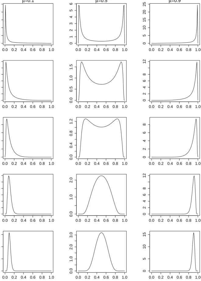
Figure 3.1 provides plots of the probability density functions for simplex distributionS2(µ, λ)
with µ= (0.333,0.333,0.334) and various λ’s.
3.2.6
Multivariate simplex GLM
Suppose the response of the i-th subject yi = (yi,1,· · · , yi,m−1) follows multivariate
sim-plex distribution Sm−1(µi, λ), where µi = (µi,1,· · · , µi,m−1) and i = 1,· · · , n. We use the
multivariate logit link to formulate the systematic component
ηi = logµi,1 µi,m log µi,2 µi,m .. . log µi,m−1 µi,m = XTi 0 0 · · · 0 0 XTi 0 · · · 0 .. . ... . .. ... ... 0 · · · 0 XTi 0 0 · · · 0 0 XTi β1 β2 .. . βm−1 =XTi β,
where µi,m = 1−Pm
−1
j=1 µi,j,ηi = (ηi,1,· · · , ηi,m−1)T, xi = (1, xi,1,· · · , xi,p−1)T, i= 1,· · · , n,
βj = (βj,0, βj,1,· · ·, βj,p−1)T, j = 1,· · · , m−1 and 0= (0,· · · ,0)1×p.
The score function U(β) for the regression parameter β is
n X i=1 ∂li ∂β = n X i=1 ∂ηi ∂β ∂µi ∂ηi ∂li ∂µi = n X i=1 Xi ∂µi,1 ∂ηi,1 · · · ∂µi,m−1 ∂ηi,1 .. . · · · ... ∂µi,1 ∂ηi,m−1 · · · ∂µi,m−1 ∂ηi,m−1 ∂li ∂µi,1 .. . ∂li ∂µi,m−1 , where ∂µi,j/∂ηi,j0 = µi,j(1−µi,j) if j =j0, −µi,jµi,j0 if j 6=j0.
and∂li/∂µi,j is given as (3.2.8),i= 1,· · · , n andj = 1,· · · , m−1. The Fisher’s information
I(β) in terms of β is n X i=1 ∂ηi ∂β ∂µi ∂ηiACov yi −1 AT ∂µi ∂ηi T ∂ηi ∂β T .
We implement the Fisher-scoring algorithm in the search of the MLE ˆβ ˆ
βk+1 = ˆβk+I−1( ˆβk)U( ˆβk).
At each iteration step, the dispersion parameter λ in the above equation is replaced by ˆ
λ= Pnn(m−1)
i=1D(yi,µˆi)
,
which is a consistent estimator of λ. In fact, following the result of Lemma 1 that 1
λ = 1
m−1E(D(yi;µi)),
Pn
i=1D(yi,µi)/n(m − 1) is a consistent estimator of 1/λ, and then by the Continuous
Mapping Theorem n(m−1)/Pn
Chapter 4
Simulation Studies for Multivariate
Simplex Models
As illustrated previously, we are interested in comparing the multivariate simplex model and the logit-normal model. So in this chapter, we assess these two models’ performance when the real data are either multivariate simplex distributed or logit-normal distributed by simulation studies.
4.1
Generating random vectors from multivariate
sim-plex distribution
In order to conduct simulation studies, we need to generate data distributed from multivari-ate simplex distribution and logit-normal distribution. Generating logit-normal distributed random vectors is straightforward but generating data from multivariate simplex distribu-tion is more difficult. In this secdistribu-tion, we propose a method to generate composidistribu-tional data from multivariate simplex distribution by conditioning.
Suppose we would like to generate a random vector y = (y1, y2, . . . , ym−1) from a
multi-variate simplex distribution Sm−1(µ, λ). Denote the conditional distribution function of yi
given (y1, y2, . . . , yi−1) asFi(yi|y1, y2, . . . , yi−1), and denote the marginal distribution function
of yi as Fyi(yi). The algorithm for generating a random vector y with multivariate simplex
distribution Sm−1(µ, λ) is
1. Generate y1 with distribution functionFy1.
2. Generate y2 with distribution functionF2(·|y1).
3. Generate y3 with distribution functionF3(·|y1, y2).
.. .
m−1. Generate ym−1 with distribution functionFm−1(·|y1, y2, . . . , ym−2).
m. Return y= (y1, y2, . . . , ym−1).
By (3.2.5), the marginal distribution Fy1 is
S1 µ1, λ m Y i=1 µi !−2/(m−1) [µ1(1−µ1)]2 .
For any k= 1, . . . , m−2, by (3.2.4) and (3.2.3), ´ y 1−y˜+ ˜ y+∼Sm−k−1( ´ µ 1−µ˜+ , λ4), where λ4 = λ 1−y˜+ m Y i=1 µ−i 2/(m−1) m Y i=k+1 µi2/(m−k−1)·(1−µ˜+)−2/(m−k−1).
Therefore, the conditional distribution of yk+1 given ˜y is
yk+1 1−y˜+ ˜ y∼S1( µk+1 1−µ˜+ , λ♦), (4.1.1)
where λ♦ = λ 1−y˜+ m Y i=1 µ−i 2/(m−1)·µ2k+1(1−µk+1−µ˜+)2(1−µ˜+)−2.
Using the above results on the marginal and conditional distributions of components of Sm−1(µ, λ), we could generate the multivariate simplex distributed random vector by
component as long as we could generate univariate simplex distributed random variable. The R function rsimplex developed by Yee (2012) in the package VGAM will be used to generate univariate simplex data.
4.2
Compare multivariate simplex models with
multi-variate logit-normal models
4.2.1
Case I: multivariate simplex models are the true models
In this section, we examine how the multivariate simplex model and the multivariate logit-normal model perform when the data are generated from the former. For simplicity, we focus on the case when m = 3. Specifically, we generate independent compositional outcomes yi = (yi1, yi2) from S2(µi, λ) with µi related to the covariatexi through
logµi1 µi3 logµi2 µi3 = β10+β11xi β20+β21xi
fori= 1, . . . , n. The covariatexi is a binary variable generated from a Bernoulli distribution
B(0.4), that is, Pr(xi = 1) = 0.4. The true values of the regression parameters are set as
β10= 0, β11 =−0.5,β20 = 0, β21= 0.5 and the dispersion parameter λ = 0.01,0.05,0.1,0.5,
and 1. Sample sizentakes value 100 or 1000. For each setting, 1000 data sets were generated and a multivariate simplex model and a logit-normal model were fit for each data set.
An intuitive thought is to compare which model yields parameter estimates that are closer to the true values. This is the method adopted by Song (2007). Table 4.1 tabulates the estimates of β and its standard deviation, and the estimated standard errors from the asymptotic distribution of ˆβ.
As we can see, in all cases, the estimates based on the multivariate simplex model are closer to the true parameter values than the estimates based on the multivariate logit-normal model, and the standard deviations are smaller than those based on multivariate logit-normal model. The smaller theλ, indicating larger variation in the data, the better the performance of the simplex model. For the slope parameters β11 and β21, the estimates based on
logit-normal model are much further away from the true values than the estimates based on simplex model. As λ gets larger, for example when λ = 1, the difference between the two models gets smaller. As shown in the pdf plots, whenλgets smaller, the data becomes highly skewed toward the edges of the simplex support, causing difficulty in parameter estimation under both models although the simplex model is still better. The above observations are in agreement with the ones made by Song (2007) for the univariate case.
Unfortunately, the above comparison is not fair because the β’s in the two models are different. In the multivariate simplex model we assume
log E(yi1) E(yi3) =β10+β11xi, log E(yi2) E(yi3) =β20+β21xi,
while in the multivariate logit-normal model we assume E log yi1 yi3 =β10∗ +β11∗ xi, E log yi2 yi3 =β20∗ +β21∗ xi.
Since the left-hand sides of the two sets equations are not equal, we know that generally βij 6= βij∗ for i = 1,2 and j = 0,1. So although the simulation results we discussed earlier
T able 4.1: Comparisons on parameter estimation when data are m ultiv ariate simplex distributed β10 (0) β11 ( − 0 . 5) β20 (0) β21 (0 . 5) λ n mean sd se mean sd se mean sd se mean sd se 0.01 100 -0.0053 0.1442 0.1381 -0.4958 0.2227 0.2166 -0.0068 0.1446 0.1381 0.5192 0.2318 0.2220 a -0.0102 0.3477 0.3386 -0.9525 0.5431 0.5368 -0.0039 0.3495 0.3260 0.9353 0.5226 0.5170 1000 0.0027 0.0429 0.0436 -0.5036 0.0659 0.0682 0.0009 0.0415 0.0436 0.4967 0.0684 0.0698 0.0142 0.1080 0.1078 -0.9858 0.1696 0.1704 0.0089 0.1048 0.1041 0.9072 0.1593 0.1646 0.05 100 -0.0009 0.1251 0.1255 -0.5109 0.1997 0.1981 0.0051 0.1287 0.1254 0.4909 0.1903 0.1958 0.0067 0.2119 0.2093 -0.7682 0.3458 0.3318 0.0182 0.2154 0.1982 0.6618 0.2939 0.3143 1000 0.0052 0.0384 0.0397 -0.5084 0.0594 0.0625 0.0062 0.0378 0.0397 0.4887 0.0616 0.0619 0.0124 0.0627 0.0670 -0.7645 0.1015 0.1059 0.0137 0.0616 0.0632 0.6656 0.0965 0.0999 0.10 100 0.0031 0.1138 0.1136 -0.5126 0.1806 0.1804 0.0058 0.1182 0.1136 0.4912 0.1707 0.1736 0.0098 0.1614 0.1627 -0.6844 0.2589 0.2579 0.0155 0.1688 0.1524 0.5969 0.2319 0.2417 1000 0.0060 0.0347 0.0361 -0.5111 0.0558 0.0571 0.0065 0.0352 0.0360 0.4880 0.0558 0.0550 0.0096 0.0490 0.0521 -0.6834 0.0832 0.0824 0.0117 0.0492 0.0488 0.5991 0.0757 0.0771 0.50 100 0.0042 0.0740 0.0729 -0.5072 0.1213 0.1180 0.0024 0.0754 0.0729 0.4987 0.1082 0.1066 0.0055 0.0825 0.0829 -0.5586 0.1358 0.1313 0.0029 0.0839 0.0760 0.5300 0.1187 0.1206 1000 0.0028 0.0238 0.0232 -0.5056 0.0381 0.0375 0.0028 0.0233 0.0232 0.4961 0.0348 0.0339 0.0032 0.0267 0.0265 -0.5575 0.0432 0.0418 0.0032 0.0259 0.0244 0.5280 0.0385 0.0385 1.00 100 0.0031 0.0556 0.0554 -0.5038 0.0924 0.0902 0.0019 0.0569 0.0554 0.5012 0.0834 0.0800 0.0036 0.0588 0.0599 -0.5317 0.0986 0.0949 0.0020 0.0600 0.0548 0.5182 0.0874 0.0870 1000 0.0027 0.0187 0.0177 -0.5039 0.0288 0.0287 0.0022 0.0184 0.0177 0.4975 0.0251 0.0255 0.0028 0.0198 0.0192 -0.5318 0.0306 0.0303 0.0023 0.0195 0.0176 0.5145 0.0265 0.0278 a Shaded ro ws are results b as ed on m ultiv ariate simplex mo del; un sh aded ro ws are based on m ultiv ariate logit-normal
in this section suggests that the multivariate simplex model does a decent job, it does not necessarily prove that the multivariate logit-normal model is inferior.
We propose three methods to achieve a fairer comparison. The first method is based on mean square error (MSE). We note that although the β’s are different for the two models, they share one common set of parameter µ for any fixed covariate. Therefore, it is fair to compare the MSE of the estimators in estimating the parameter µ.
From the simulation setting, we know the true µ’s in group x= 0 and x= 1, µ0 = (µ01, µ02, µ03) = (0.3333,0.3333,0.3333),
µ1 = (µ11, µ12, µ13) = (0.1863,0.5065,0.3072).
Under the simplex model,µ0 and µ1 are estimated as
c
µ0 = (edβ10, edβ20,1)/(eβd10+edβ20+ 1),
c
µ1 = (edβ10+dβ11, eβd20+dβ21,1)/(edβ10+dβ11+edβ20+dβ21+ 1).
Under the logit-normal model, estimators µf0 and µf1 have no closed forms but can be es-timated based on ˆβ∗ and ˆσ2 in the logit-normal model. The MSE of µc0 is defined as E(µc0−µ0)T(µc0−µ0) and is estimated based on 1000 simulation runs. The MSE of µf0,
c
µ1, and µf1 can be similarly defined and estimated. The estimated MSE’s based on the two models are summarized in Table 4.2.
Table 4.2: Comparing the estimated MSE when data are multivari-ate simplex distributed
λ n= 100 n = 1000 0.01 0.0421 0.0505 0.0125 0.0153a 0.1002 0.1870 0.0319 0.1717 0.05 0.0367 0.0434 0.0113 0.0132 0.0621 0.0990 0.0188 0.0854 0.10 0.0341 0.0382 0.0104 0.0120 0.0488 0.0709 0.0148 0.0568 0.50 0.0217 0.0227 0.0070 0.0072 0.0244 0.0289 0.0078 0.0181 1.00 0.0165 0.0178 0.0054 0.0053 0.0175 0.0207 0.0057 0.0103
aShaded rows are results based on multivariate simplex model; unshaded
rows based on logit-normal model
As shown in Table 4.2, the simplex model produces better estimators of mean composition µthan the logit-normal model disregard the sample size or the value ofλ. And the advantage of simplex model increases asλdecreases. For examples, in the case ofλ= 0.01 andn= 1000, the estimated MSE of µ1 under the logit-normal model is 9 times larger than the one under the simplex model.
The second method we propose is to assess the power of the two models in testing certain common hypothesis. In our simulation setting, the null hypothesis of no group effect H0 :µ0 =µ1 can be tested in both models. Under the simplex model, it is equivalent to
while under the logit-normal model, it is equivalent to H0 :β11∗ =β
∗
21 = 0.
Denote the estimated covariance matrix of βc1 = (βc11,βc21) as Σc1 based on the simplex
model, then underH0,T =βc1
T
c
Σ1
−1
c
β1 follows asymptoticallyχ2 distribution with 2 degrees
of freedom. So the asymptotic test of size 0.05 rejects theH0whenT >5.9915. The power of
this test is estimated using 1000 simulations. The power of the test under the logit-normal model is estimated similarly. In addition, we also conducted the matching simulation to estimate the type I error rate under each model (Table 4.3).
Table 4.3: Comparisons on powers and type I errors when data are multivariate simplex distributed (alternative: β= (0,−0.3,0,0.3))
n= 100
λ Power Type I error 0.01 0.710 0.063a 0.482 0.060 0.05 0.774 0.057 0.662 0.066 0.10 0.845 0.056 0.762 0.060 0.50 0.997 0.044 0.994 0.048 1.00 1.000 0.059 1.000 0.059
aShaded rows are results based on multivariate simplex model, and unshaded
The estimated type one error rate under the two models are similar disregard the value of λ and both are slightly inflated, probably due to inadequate sample size. The χ2-test based on the simplex model is more powerful than the test based on the logit-normal model, particularly when λ is small.
Finally, as the third method, we propose to compare the two models by a criterion pro-posed by Takeuchi (1976) in estimating the Kullback-Leibler distance between the working model and the true model. This criterion is known as Takeuchi Information Criterion (TIC) and is defined as TIC = 2tr( ˆQ−1Ωˆ)−2l(ˆθ), where ˆ Q=−1 n n X i=1 Hl(θ|yi,xi) θ=ˆθ and Hl(θ|yi,xi) = ∂ 2
∂θ∂θ0l(θ|yi,xi) is the Hessian matrix of l(θ|yi,xi) and
ˆ Ω= 1 n n X i=1 ∂ ∂θl(θ|yi,xi) ∂ ∂θl(θ|yi,xi) T θ=ˆθ .
TIC is a generalization of AIC which does not require that the assumed models contain the true model.
To obtain TIC, we need to calculateHl(θ|yi,xi),i= 1,· · ·, n. For simplicity, we denote
l(θ|y,x) as l(θ) in the derivation. When the multivariate simplex model is the assumed model, θ = (β, λ) and Hl(θ) = Hl(β) ∂∂β2∂λl ∂2l ∂β∂λ T ∂2l ∂λ2 .
In the last row/column,
∂2l ∂β∂λ = ∂η ∂β ∂µ ∂η ∂2l ∂µ∂λ,
where ∂η/∂β =X and ∂µ/∂η is given previously. The i-th component of ∂2l/∂µ∂λ is
∂2l ∂µi∂λ =−1 2 m Y i=1 µi !m−−21 " −2 m−1 1 µi − 1 µm m X i=1 µ2 i yi −1 ! + 2µi yi − 2µm ym # ,