Discussion Papers in Economics
No. 2000/62
Dynamics of Output Growth, Consumption and Physical Capital
in Two-Sector Models of Endogenous Growth
by
Department of Economics and Related Studies University of York
No. 2006/20
Data Driven Likelihood Ratio Tests for Goodness-to-Fit
with Estimated Parameters
by
Patrick Marsh
Data Driven Likelihood Ratio Tests for
Goodness-of-Fit with Estimated Parameters
Patrick Marsh
Department of Economics
University of York
Heslington, York
YO10 5DD
tel. +44 1904 433084
fax +44 1904 433759
e-mail: [email protected]
3
rdOctober 2006
Abstract
This paper generalizes the goodness of fit tests of Claeskens and Hjort (2004) and Marsh (2006) to the case where the hypothesis specifies only family of distributions. Data driven versions of these tests are based upon the Akaike and Bayesian selection criteria. The asymptotic distributions of these tests are shown to be standard, unlike those based upon the empirical distribution function. Moreover, numerical evidence suggests that under the null hypothesis performance is very similar to tests such as the Kolmogorov-Smirnov or Anderson-Darling. However, in terms of power under the alternative, the proposed tests seem to have a consistent and significant advantage.
1
Introduction
Recently two papers, Claeskens and Hjort (2004) and Marsh (2006) have introduced new nonparametric likelihood ratio goodness-of-fit tests. Those tests are essentially based upon Portnoy’s (1988) test applied in the context of an exponential series density estimator. The given tests are then the likelihood ratios of that nonparametric estimate to either a specified parametric density, in Claeskens and Hjort (2004), or the entropy minimizing approximate density, in Marsh (2006). There, as here, the choice of dimension of the approximate density is data driven via the selection criteria of Akaike (1974) and Schwarz (1978).
This paper extends the application of this testing principle to the general case in which only the general form of a family of distributions is hypothesized, with the parameters of that family unspecified. The most commonly used tests in this circumstance are those based upon the empirical distribution function (edf), such as the Kolmogorov-Smirnov (KS) and Cramér-von Mises (CM) procedures. However, it is well known that tests based on the edf are generally not asymptotically pivotal.
Indeed, as is clear from the analysis of Stephens (1976) and more recently Babu and Rao (2004), the asymptotic distribution of such tests may depend not only upon the hypothesized family of distributions, but also upon the particular parameters of that family. For example, simply to cover all permutations in the Gaussian family four sets of critical values are required, see Stephens (1974, 1976). Further critical values are required for other commonly tested families such as the Gamma (see Pettitt (1978)), the special cases of the Exponential with unknown mean (Lilliefors (1969)) and also with unknown mean and scale (Spinelli and Stephens (1987)).
The test considered in this paper is shown to be, under standard regularity condi-tions, asymptotically pivotal. That is the asymptotic distribution is the same within and across different hypothesized families. Moreover the asymptotics involved are standard. When appropriately standardized, with respect to the dimension of the approximating exponential, the test is asymptotically standard normal. Thus the
asymptotic distribution applies in all relevant cases, unlike that for edf based sta-tistics. It is also straightforward to establish that the test is consistent against any
fixed alternative. The paper also contains an exhaustive numerical study in which it is shown that the size properties of a version of the new test are very similar to those tests based on the edf. However, for cases involving both the Gaussian and Exponential null hypotheses the new test has a significant relative power advantage.
2
Preliminaries
Suppose that our sample y= {yi} n
i=1are i.i.d. copies of a random variable Y having
distribution
Pr[Y ≤y] =F(y),
and we wish to test the goodness-offit hypothesis
H0 :F(y) =F(y;β), (1)
whereF(., .)is specified up to the unknownk×1vectorβ.Letβˆndenote the maximum likelihood estimator (mle) for β based upon the sample y.
To proceed consider the (possibly composite) function h = h(y;β) : R×Rk → (0,1) and suppose that the following assumption holds:
Assumption 1 :
i) The mle is uniformly consistent and √
n(ˆβn−β) =Op(1) (2)
ii) Let Hi(β) =∂h(Yi;β)/∂β and let B be a ball of radius ε/√n for ε >0, then
lim n→∞supβ∈B|
Hi(β)|≤c < ∞ for all i= 1, .., n (3)
On the basis of Assumption 1, if we define
xi =h(yi; ˆβn),
then from a mean value expansion forh(Yi, .)
h(yi; ˆβn) =h(yi;β) + ˆβn−β Hi(β∗i),
for each mean valueβ∗i lying on a line segment joining βˆn andβ. We can write
xi =hi +ei,
where xi is as above, hi = h(yi;β) is an i.i.d. random variable, having density q(h),
say, and from (2) and (3) of Assumption 1
ei =ei(F, h,β∗i) =Op(n−1/2),
so the ei are degenerate random variables depending upon the distribution F, the
functionh and the valueβ∗.By constructionh∈(0,1),so that the random variables
xi, hi andei are bounded as in
xi, hi ∈(0,1) ; ei ∈(−1,1). (4)
To proceed we shall define three vectors of raw sample moments up to and includ-ing themth lying in the sample space Φ
⊂Rm, with ¯ x=n−1 n i=1 xji m j=1 , ¯h=n−1 n i=1 hji m j=1 and e¯=n−1 n i=1 eji m j=1 . (5) Analogously we can also define the population moments corresponding to these ran-dom variables as ξ = ξj m j=1 ; ξj = n i=1E[(xi) j ] n ≤ ∞ η = ηj m j=1 ; ηj =E[(hi) j ]≤ ∞ ε = {εj}mj=1 ; εj = n i=1E[(εi) j ] n ≤ ∞, (6)
3
The Density Estimator
The properties of the exponential series density estimator werefirst detailed by Crain (1974), and refined and extended by Barron and Sheu (1991). Suppose that we have
n observations on the i.i.d. hi (for the purposes of this exposition we will simply
assume that the density q(h),defined on (0,1),satisfies the conditions of Barron and Sheu (1991)). The exponential series density estimator of the density q(h) is the maximum likelihood estimator in the (infinite) exponential family,
ph(θ) = exp m
j=1
θjφj(h)−ψm(θ) , (7) where Θ is the m dimensional parameter space, the φj(.) are linearly independent
functions spanning Rm and the cumulant functionψm(θ) is given by ψm(θ) = ln 1 0 exp m j=1 θjφj(h) dh.
For the sampleh= (h1, .., hn), the density estimator is defined by
ph(ˆθ) = lim m,n→∞, m/n→0θ∈supΘ⊂Rm exp m j=1 θj n i=1 φj(hi)−nψm(θ) . (8)
Although there are a number of different choices for the functions φj(.) for simplicity
we will assume that they are polynomials. The difference between the set-up here and that of the papers by Crain (1974) and Barron and Sheu (1991) is that we don’t observe the hi, but instead the xi. We will also explicitly choose a polynomial basis
with
φj(h) =hj.
As Marsh (2006) details, choosing polynomials over say trigonometric series has little numerical effect, in the known parameter case. Since, as far as the estimator itself is concerned, the effect of estimating nuisance parameters has only a small impact upon its numerical accuracy, according to evidence presented below, the same is true in this case also.
To apply the exponential series density estimator, note that the mle ˆθ given in (7) can be written as the solution to a set of m equations, as in
1
0
hjph ˆθ dh= ¯h ; j = 1, .., m. (9)
Analogously, and since the law of large numbers impliesn−1 n i=1h j i →p η0j,then we can define a value θ0 by 1 0 hjph(θ0)dh=η0 ; j = 1, .., m, (10) with η0 = η0j m
j=1 and ph(θ0) is the minimum entropy estimator for p(h) in the
exponential family. Finally, since in fact we observe {xi} n
1, then we define the value
˜ θ by
1
0
hjph ˜θ dh = ¯x. (11)
Importantly, given the values¯h, η andx¯ inRm the parameter valuesˆθ,θ
0 and˜θ, are
uniquely determined via the convexity of the exponential likelihood, see Barron and Sheu (1991).
To detail the asymptotic properties of the estimated densityph ˜θ , suppose that
we have chosen h so that the log-density lp(h) = log[p(h)] has r − 1 absolutely continuous derivatives and that its rth derivative, drlp(h)/dhr is square integrable, i.e. so that lp(h) ∈ Wr
2, the Sobolev space of functions on [0,1]. Also define the
relative entropy for two densities p1 and p2 by
D[p1|p2] = 1 0 ln p1(h) p2(h) p(h)dh, then:
Theorem 1 Let ˜θ denote the estimated exponential parameter determined by (11) and suppose that the conditions in Assumption 1 are met, then
Theorem 1, proved in Appendix I, demonstrates that in terms of the density estimator itself the effect of observing{xi}
n
1 rather than{hi} n
1 is asymptotically
neg-ligible, provided that the conditions of Assumption 1 are met. The rate of convergence of the estimator in the simpler case is at least of orderOp n−
2r
1+2r whenm is chosen
optimally so thatm ∝n1+21r.It should not be surprising that the rate of convergence
is unaffected when parameters are replaced by√n uniformly consistent estimators. In the following section the details of the proposed nonparametric likelihood ratio test will be given along with it’s asymptotic distributions under both the null and alternative.
4
The Likelihood Ratio Test
As in the simpler goodness-of-fit case the proposed test is the likelihood ratio test of Portnoy (1988) applied via the density estimator of Crain (1974) and Barron and Sheu (1991). That is, we replace the goodness of fit hypothesis, with one within the (infinite) exponential family (7) i.e.,
H0 :F(y) =F(y;β)⇒H0 :h∼ lim
m→∞P(θ0), (12)
where ph(θ0) = dP(θ0) and θ0 is the solution to (10). It is important to note that
P(θ0) represents the distribution of the transformed observations x=h(y,β).
How-ever, given observations on{xi}n1 rather than the unobserved {hi}n1 Portnoy’s (1988)
test becomes Λm = 2 log px ˜θ px(θ0) = 2n ˜θ−θ0 x¯− ψm ˜θ −ψm(θ0) , (13)
where ˜θ is the solution to (11).
For every alternative distribution for Y there is a unique alternative distribution forhon(0,1)and associated with that distribution will be another consistent density
estimator given by say, ph(θ1). In practice, of course, θ1 will neither be known nor
specified. None-the-less, as with analogous tests in the parametric exponential family, (12) will be rejected for large values of Λm.
The following Theorem, again proved in the appendix gives the asymptotic dis-tribution of the likelihood ratio test statistic both under the null hypothesis (12) and also demonstrates consistency against fixed alternatives.
Theorem 2 Suppose that we construct {xi} n
i=1 as described above and that the
con-ditions required in Assumption 1 are met, then
(i) Under the null hypothesis H0 :h∼limm→∞P(θ0),
lim m,n→∞;m=o(n1/3)
Λm−m
√
2m ∼N(0,1) +op(1). (14)
(ii) Under any complementary alternative H1 :h ∼Q=P(θ0), then for any critical
value kα of sizeα<1 lim m,n→∞;m=o(n1/3) Pr Λm−m √ 2m ≥kα = 1. (15)
Theorem 1 applies for any distribution of Y satisfying Assumption 1 and any function h(y;β) which has a density satisfying the conditions of Barron and Shue (1991). Consequently, the asymptotic distribution of the test is the same both across and within families of distributions. This is not so for those tests based on the edf.
As with the simplest case considered in Claeskens and Hjort (2004) and Marsh (2006) it is possible to demonstrate the existence of power against local alternatives of the form H0 : lim m→∞h∼P(θ1) ; θ1 =θ0+c √ m n , c c =O(1).
However, since in this more general case the precise parameter values are irrelevant ascribing significance to such alternatives is difficult. More important will be the comparative numerical properties of the test, as described in the following section.
Before proceeding, as with the tests in both Portnoy (1988) and Marsh (2006), an approximation based upon (14), but utilizing the Chi-square distribution, as in,
lim
m,n→∞;m=o(n1/3) Λm ∼χ
2(m),
will prove a more relevant approximation in finite samples. Moreover, in practical applications the remaining unresolved issue remaining is the choice of m.
Here we will employ the data driven model selection criteria of Akaike (1974) and Schwarz (1978). To implement these, define the set of integersM={1,2, ...,m¯},and let the estimated dimensions based upon these criteria bemˆA and mˆB, respectively,
which satisfy ˆ mA = arg max m∈M logpx ˜ θ −m ˆ mB = arg max m∈M logpx ˜ θ −mlogn . (16) As with the simpler case either criteria will deliver a consistent density estimator in the sense that if we allow m¯ to grow but satisfying m¯ =o(n1/3), then both mˆ
A and ˆ
mB will diverge. Although in a finite familymˆA will over-fit, this is not possible in
this, asymptotically, infinite family.
5
Numerical Properties
5.1
Properties of the density estimator with estimated
para-meters
Before detailing the goodness-of-fit test in this circumstance we can enumerate pre-cisely the effect that having to estimate unknown parameters has on the series density estimator of Crain (1974). The Kullback-Leibler distance (or relative entropy) from the true density q(h) to the estimated densityph(˜θ)may be fully decomposed as
While thefirst term in (17) may be evaluated explicitly, the last two instead need to be simulated. To proceed consider two experiments,
(i): Y ∼Exp(1) and (ii): Y ∼N(0,1),
and define hi = 3 F(yi;β) ; xi = 3 F(yi; ˆβ), (18)
where F(y,β) is the distribution function of either case (i) or (ii) and βˆ is the max-imum likelihood estimator of the parameters of that distribution on the basis of the sample {xi}n1. Choosing the cube root in (18) implies that the density of h is
q(h) = 3h2.Given this density for any dimensionmthe unique vectorθ
0 can be found
via (10). From that density the distanceD[p(h)| ph(θ0)]can be explicitly calculated,
the values for which are given in Table 1a. Notice that from a purely numerical per-spective there is very little to be gained from choosing dimensions greater than say
m= 5.
Given samples {hi}n1 and {xi}n1 the respective estimators ˆθ and ˜θ can be
deter-mined from (9) and (11). From the associated density estimators the quantities
D[ph(θ0)| ph(ˆθ)]andD[ph(ˆθ)| ph(˜θ)]can then be calculated. Replicating these 5000
times over both experiments, for four samples sizes of n = 50,100,200,400 and for dimensions of m = 1,2,3,4,5, these distances can be numerically evaluated via the Monte Carlo sample averages of the replicated distances.
These values are presented in Tables 1b (for experiment (i)) and 1c (for (ii)). From Table 1 it is clear that the overwhelmingly significant contribution to entropy, in (17), is D[ph(θ0)| ph(ˆθ)] which measures our ability to estimate the approximate density
ph(θ). Both our ability to approximatep(h)with ph(θ) and the effect to of having to
estimateβ, i.e. using ˜θ rather than ˆθ has a relatively small numerical impact. Thus we may concentrate on providing tests with good statistical properties, i.e. size and power, rather than on the basis of the density estimator itself.
5.2
Size and power properties
In this subsection we shall contrast the finite sample numerical behaviour of the proposed tests based on (13) with those commonly used tests based upon the edf, specifically the KS, CM and Anderson-Darling (AD) tests. These tests are given in either Stephens (1976) or Conover (1999), along with the relevant critical values for all the cases considered here. All of the experiments in this section are based upon the following procedure. The variables{yi}
n
i is generated from a particular distribution,
F(y;β), while samples lying in(0,1)are then constructed from
xi =
3
F(yi; ˆβ),
so that the relevant density is q(h) = 3h2. For a given m, the test statistic Λm is
constructed as described above.
The first set of experiments (based upon 5000 replications and for sample sizes of
n= 100,200,400) concern testing the respective null hypotheses,
H0a : Y ∼Exp[µa], H0b : Y ∼N(µb,σ2),
where µa, µb and σ2 are to be estimated. Here we shall first consider the impact
of choosing different values of m for the approximation. Data were generated using specified values of µa = 1, µb = 0 and σ2 = 1. Tables 2a and 2b give the rejection
frequencies of asymptotic critical values, at both the 5% and10% significance level, based upon theχ2(m)approximation forΛm and based upon tabulated values for the
KS, CM and AD tests. Naturally, different critical values are required for the latter three tests for each of the hypotheses. For hypothesis Ha
0 the values of m = 6,9,12
were chosen while forH0b, m= 6,9,12,15are used.
Two salient points are worth highlighting from Table 2. First it is clear that there are versions of the new test which have very similar size properties to those of the commonly used tests. Second is that to achieve that, the dimension m needs to be
quite large. This is particularly so for the second hypothesis, which involves an extra parameter to be estimated. Indeed for these cases, on the sole basis of finite sample size, it is necessary that m is larger than for the simpler hypotheses considered in Claeskens and Hjort (2004) and Marsh (2006). Commensurate with that is that the approximation is acceptable only for large sample sizes.
From the numerical work of Marsh (2006) and also that to be presented below, both of the data driven selection criteria in (16) tend to favour model dimensions significantly below those delivering acceptable finite sample size performance. Con-sequently, we shall also employ a numerical correction to the resulting statisticsΛmˆA
andΛmBˆ , based upon the principle of Bartlett correction. For a given familyF(y;β)
and sample sizen we can construct an estimator of the mean of Λm via re-sampling
from y˜i ∼ F(y; ˆβ) where βˆ is the estimator obtained from {yi}n1. Resampling say R
times and constructing {Λm,r}Rr=1we define, for any m, υm,R= 1
R
R
r
Λm,r,
so that as n → ∞, βˆ →p β and as R → ∞, limmυm,R →p limm,nE[Λm] = m.
Consequently, we can construct a numerical Bartlett-type correction, giving
m Λm υR −1
√
2m →d N(0,1),
and with a Chi-square approximation
lim m,n→∞;m=o(n1/3) ¯ Λm = mΛm υR ∼χ 2(m). (19)
It is important to note that no higher-order claim is being made for the approximation in (19). Moreover, the resampling scheme proposed is not a Bootstrap. Specifically
υR need only be calculated once within any family F(y;β), for each m. Thus the computational burden is very low compared to a scheme which would resample for each replication of a simulation study. Although such schemes have been suggested, for example in Janssen, Swanepoel and Veraverbeke (2005), they were not actually
applied. Moreover, the evidence here suggests that such schemes, and the computa-tional cost involved, are not necessary in order to get acceptable behaviour under the null hypothesis.
Consequently, all further experiments are performed on the basis of choosing the dimension m via (16), optimizing over M = {1,2,3,4} and correcting the resulting statistics via (19) with R = 250. For each family, each correction factor υm,R took between 1 and 2 minutes to compute on a Pentium IV 3.0Ghz. The experiments presented in Tables 3a and 3b are entirely analogous those presented in Tables 2a and 2b, excepting that the sample sizes are now n = 25,50 and 100. Tables 4a and 4b repeat these experiments but with data generated by Exp[5] and N[1,2]
random variables, respectively. Once again the tables indicate that the new test, albeit with this numerical Bartlett-type correction, has size broadly comparable with those commonly used tests. In fact for small samples perhaps the new tests performs slightly better, particularly so compared to the KS test. In addition there is nothing to choose between either of the dimension selection criteria.
The final set of experiments concern the relative power of all of the tests. First we shall test
H0 :Y ∼Exp[1] vs. H1 :Y ∼Γ(v,1),
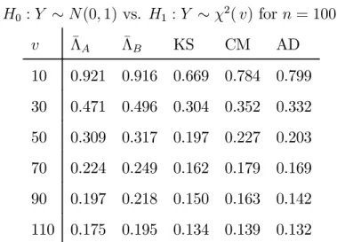
where Γ(v,1) denotes a Gamma random variable. Values for values of v ranging from −1.44 to 0.56 were used, with the null hypothesis implying that v = 1. Fixing the sample size at 100, simulated critical values were taken from the experiments used to generate Table 2a. Then those experiments were repeated, but with the data generated under the alternative hypothesis. The rejection frequencies of those simulated critical values are recorded in Table 5. Similar experiments were conducted for tests of H0 :Y ∼N(0,1) vs. Ha 1 :Y ∼χ2(v)−v H1b :Y ∼t(v) , where χ2(v)
−v and t(v) are centered Chi-square and Student-t random variables, respectively. Rejection frequencies under the alternatives are presented in Tables 6a
and 6b, respectively, for ranges of values ofv.
Under these alternatives there are now significant differences in the performances of the tests. While there is still nothing to choose between the dimension selection criteria, either produces a new test which is significantly more powerful than any of those based upon the empirical distribution function.
6
Conclusions
This paper has extended the nonparametric likelihood ratio goodness-of-fit tests of Claeskens and Hjort (2004) and Marsh (2006) to cover all cases involving estimated parameters. Specifically it has been demonstrated that having to estimate unknown parameters does not affect the rate of convergence of either the density estimator of Crain (1974) and Barron and Sheu (1991), nor of the associated likelihood ratio test of Portnoy (1988). Moreover it is therefore straightforward to so that the new test has an asymptotic distribution which depends upon neither the family being tested, nor the particular member of that family. Thus the test has significant theoretical advantages over those based upon the empirical distribution function.
Numerical evidence suggests that the impact of having to estimate parameters on the density estimator is quite negligible. In terms of the associated new test, initially it was found that the dimension of the model needed to be quite large in order that asymptotic critical values had usable finite sample properties. In order to deliver a more practical procedure data driven dimension selection criteria were employed. Utilizing a very simple and efficient numerical correction practical versions of the new test were demonstrated to have very competitive performance under different null hypotheses. Moreover, under relevant alternatives the new tests were shown to be significantly more powerful.
References
Akaike, H. (1974). A new look at the statistical model identification. System
identi-fication and time-series analysis. IEEE Trans. Automatic Control AC-19, 716—723 Anderson, T.W. (1962). On the distribution of the two-sample Cramér-von Mises criterion. Annals of Mathematical Statistics, 33, 1148-1159.
Anderson, T.W. and D.A. Darling (1952). Asymptotic theory of certain ‘goodness-of-fit’ criteria based on stochastic processes. Annals of Mathematical Statistics, 23, 193-212.
Babu, G. and C.R. Rao (2004). Goodness-of-fit tests when parameters are estimated. Sankhya, 66, 63—74.
Barron, A.R. and C-H. Sheu (1991). Approximation of density functions by sequences of exponential families. Annals of Statistics, 19, 1347-1369.
Claeskens, G. and N.L. Hjort (2004). Goodness of fit via nonparametric likelihood ratios. Scandinavian Journal of Statistics, 31, 487-513.
Conover, W.J. (1999). Practical Nonparametric Statistics, John Wiley and Sons, New York.
Crain, B.R. (1974). Estimation of distributions using orthogonal expansions. Annals of Statistics, 2, 454—463.
Janssen, P., J. Swanepoel and N. Veraverbeke (2005). Bootstrapping modified goodness-of-fit statistics with estimated parameters. Statistics and Probability Letters, 111— 121.
Lilliefors, H.W. (1969). On the Kolmogorov-Smirnov test for the exponential dis-tribution with mean unknown. Journal of the American Statistical Association, 64, 387-389.
Marsh, P.W.N. (2006). Goodness offit tests via exponential series density estimation. Journal of Computational Statistics and Data Analysis, to appear.
Pettitt, A. N. (1978). Generalized Cramér-von Mises statistics for the gamma distri-bution. Biometrika, 65, 232—235.
Portnoy, S. (1988). Asymptotic behaviour of likelihood methods for exponential families when the number of parameters tends to infinity. Annals of Statistics, 16, 356-366.
Schwarz, G. (1978). Estimating the dimension of a model. Annals of Statistics, 6, 461-464.
Spinelli, J.J. and M.A. Stephens (1987). Tests for exponentiality when origin and scale parameters are unknown. Technometrics, 29, 471—476.
Stephens, M.A. (1976). Asymptotic results for goodness-of-fit statistics with unknown parameters. Annals of Statistics, 4, 357—369.
Stephens, M.A. (1974). EDF statistics for Goodness of fit and some comparisons. Journal of the American Statistical Association, 69, 730-736.
Appendix I: Proofs
In order to avoid any ambiguity throughout this appendix the order of magnitude symbol O(.)is defined by an,m=O(bn,m)⇐⇒ lim m,n→∞ ; m3/n→0 an,m bn,m ≤ c1 <∞,
and analogously for the probabilistic versions Op(.) and op(.). If the quantity
un-der scrutiny does not depend upon the dimension m then the condition m3/n
→ 0
becomes redundant.
Proof of Theorem 1:
Consider the vectors given in (5)
¯ x = 1 n n i=1 xi, ..., n i=1 xmi ¯ h = 1 n n i=1 hi, ..., n i=1 hmi ,
and the Euclidean distance between them
¯ x−¯h = 1 n n i=1 (xi−hi), ..., n i=1 (xmi −hmi ) .
Taking a typical element, the jth, and noting x i =hi+ei 1 n n i=1 xji −hji = 1 n n i=1 j s=0 j! s!(j−s!)h j−s i e s i −h j i = 1 n n i=1 j s=1 j! s!(j−s!)h j−s i e s i.
Since hi =Op(1)and hi ∈(0,1) whileei =Op(n−1/2) andei ∈(−1,1) then
hji−s =Op(1) and esi =Op(n−s/2) and so j s=1 j! s!(j−s!)h j−s i e s i =Op(n−1/2) for all j, and hence 1 n n i=1 xji −hji = 1 n n i=1 j s=1 j! s!(j −s!)h j−s i e s i =Op(n−1/2).
Consequently and from the definition of Euclidean distance we have,
¯ x−¯h = m j=1 1 n n i=1 xji −hji 2 =Op m n . (20)
Considering now the population moment vectorη,then from the triangle inequal-ity we have
|x¯−η|≤ h¯−η + ¯x−¯h =Op
m
n , (21)
which follows from (20) and the same order of magnitude applies for thefirst distance, see Barron and Sheu (1991).
Extending the decomposition of the Kullback-Leibler divergence of Barron and Sheu (1991) we obtain,
D[p(h)|ph(˜θ)] =D[p(x)|ph(θ0)] +D[ph(θ0)|ph(ˆθ)] +D[ph(ˆθ)|ph(˜θ)]. (22)
From Barron and Sheu (1991) the first two terms are, respectively, O(m−2r) and
Op(m/n). Application of Lemma 5 in Barron and Sheu (1991), which holds for any
two values in Rm, uniquely defined by equations as in (9) and (11) implies
O(D[ph(ˆθ)|ph(˜θ)]) =Op ¯h−x¯
2
=Op
m n ,
and hence O(D[p(h)|ph(˜θ)]) = O(D[p(x)|ph(θ0)) +Op m n = O(m−2r) +Op m n , as required. Proof of Theorem 2:
Part (i): To proceed we have defined
Λm = 2n ˜θ−θ0 x¯− ψm ˜θ −ψm(θ0) ,
where ˜θ solves (11), or alternatively
ψm ˜θ =
∂ψm ˜θ ∂θ
θ=˜θ
= ¯x. (23)
Similarly the valueθ0 is defined by
ψm(θ0) =η0 =E(¯h). (24)
Since the exponential log-likelihood is strictly convex then the mapping
θ(η) :ψm(θ) =η
is one-to-one between the parameter spaceΘ and sample spaceΦand application of both (5.6) of Lemma 5 in Barron and Sheu (1991) and also (21) gives
O(|˜θ−θ0|) =O(|x¯−η0|) =Op
m
n . (25)
As a consequence of both (25) and (21) we have that
O(|˜θ−θ0|) =O |ˆθ−θ0| and O(|x¯−η0|) =O |¯h−η0| .
Now let U =V −Eθ0[V], V ∼ pv(θ0), then the moment conditions (2.4) and (3.2)
of Portnoy (1988) are trivially satisfied since here the elements of V = {vj} m j=1 are
proofs of Theorem 3.1 and 3.2 apply for any two pairs of values in ˜θ,θ0 and(¯x,η0)
given the orders of error satisfy (25).
As there without loss of generality we may assume that the exponential family is parameterized such that
ψm(θ0) =η0 =Eθ0[¯h] = 0 and ψm(θ0) =V arθ0[¯h] =Im, (26)
that is it ish¯which is assumed to be standardized notx.¯ None-the-less using (23) and exploiting (26) we have expansions analogous to (3.5) and (3.6) of Portnoy (1988),
|˜θ−θ0|2 = ˜θ−θ0 x¯− 1 2Eθ0 ˜θ−θ0 U 2 +Op m2 n2 ˜ θ−θ0 x¯ = |x¯0|2− − 1 2Eθ0 ˜θ−θ0 U 2 ¯ x U +Op m2 n2 .
Then arguments identical to those giving Theorem 3.1 of Portnoy (1988) yields,
|˜θ−θ0−x¯|=Op m n , and consequently Λm = 2n ˜θ−θ0 x¯− ψm ˜θ −ψm(θ0) = n |x¯|2 −|θ˜−θ0−x¯|2+ 1 6Eθ0 ˜θ−θ0 U 3 +Op m2 n , and so λm = Λ√m−m 2m = n|x¯|2 −m √ 2m +op(1) = n|h¯+ ¯e| 2 −m √ 2m +op(1) ≤ n|h¯| 2 −m √ 2m + n|e¯|2 √ 2m +op(1) = n|h¯| 2 −m √ 2m +op(1),
the latter following since the elementsei are degenerate random variables asn→ ∞.
central limit theorem as in Portnoy given immediately the asymptotic distribution.
Part (ii): Suppose that under the fixed alternative the density of ¯h is qA(h) and
letθ1 be the unique solution to 1 0 hjph(θ1)dh= 1 0 hjqA(h)dh ; j = 1, .., m.
Now |θ0−θ1| = O(√m), while the mle is consistent for θ1 in that ˜θ−θ1 =
Op m/n . Writing, n ˜θ−θ0 x¯= √ n m j=1 (˜θj−θ0j) 1 √n n i=1 xji,
where we have put ˜θ = ˜θ1, ..˜θm and θ0 = (θ01, ..,θ0m), and noting that since the
xji are i.i.d., then for each j
1 √ n n i=1 xji =Op(1), and consequently n ˜θ−θ0 x¯=Op m √ n . (27)
Furthermore, from the definition of the exponential density ψm(θ0) is O(1), while
ψm(˜θ) is Op(1), and hence
n ψm ˜θ −ψm(θ0) =Op(n). (28)
Together (27) and (28) imply that under anyfixed alternative
Λm =Op m √ n+n , and hence lim m,n→∞;m=o(n1/3) Pr Λm−m √ 2m ≥kα = 1.
Appendix II Tables
Table 1a: Kullback-Leibler distances
m 1 2 3 4 5 6 7
D[q(h)|ph(θ0)] .0186 .0115 .0028 .0023 .0008 .0007 .0007
Table 1b: Monte Carlo Kullback-Leibler distances forY ∼Exp[1]
i)D ph(θ0)|ph(ˆθ) n 50 100 200 400 m 1 .0213 .0198 .0192 .0188 2 .0183 .0145 .0129 .0122 3 .0161 .0085 .0056 .0042 4 .0222 .0105 .0062 .0041 5 .0320 .0130 .0064 .0035 ii)D ph(ˆθ)|ph(˜θ) n 50 100 200 400 m 1 .0010 .0008 .0005 .0003 2 .0023 .0014 .0011 .0005 3 .0036 .0015 .0011 .0004 4 .0040 .0018 .0010 .0006 5 .0049 .0019 .0012 .0004
Table 1c: Monte Carlo Kullback-Leibler distances forY ∼N(0,1)
i)D ph(θ0)|ph(ˆθ) n 50 100 200 400 m 1 .0187 .0186 .0184 .0184 2 .0141 .0127 .0121 .0118 3 .0104 .0065 .0046 .0037 4 .0149 .0082 .0051 .0036 5 .0233 .0099 .0052 .0029 ii) D ph(ˆθ)|ph(˜θ) n 50 100 200 400 m 1 .0043 .0016 .0013 .0007 2 .0060 .0025 .0014 .0006 3 .0084 .0032 .0017 .0009 4 .0099 .0038 .0020 .0010 5 .0133 .0046 .0021 .0011
Table 2a: Monte Carlo rejection frequencies under Ha 0 :Y ∼Exp[1] size 0.10 0.05 n 100 200 400 100 200 400 Λ6 0.112 0.096 0.102 0.062 0.058 0.049 Λ9 0.105 0.103 0.985 0.054 0.049 0.047 Λ12 0.109 0.098 0.101 0.057 0.051 0.050 KS 0.081 0.092 0.103 0.041 0.049 0.051 CM 0.095 0.095 0.096 0.051 0.051 0.049 AD 0.093 0.095 0.100 0.050 0.051 0.049
Table 2b: Monte Carlo rejection frequencies under
Hb 0 :Y ∼N(0,1) size 0.10 0.05 n 100 200 400 100 200 400 Λ6 0.062 0.067 0.072 0.031 0.035 0.038 Λ9 0.068 0.072 0.079 0.037 0.040 0.041 Λ12 0.081 0.086 0.095 0.041 0.045 0.047 Λ15 0.095 0.096 0.099 0.043 0.047 0.049 KS 0.076 0.088 0.099 0.036 0.042 0.044 CM 0.105 0.099 0.097 0.055 0.052 0.049 AD 0.101 0.097 0.098 0.053 0.047 0.048
Table 3a: Monte Carlo rejection frequencies under H0 :Y ∼Exp(1) size 0.10 0.05 0.01 n 25 50 100 25 50 100 25 50 100 ¯ ΛA 0.098 0.099 0.102 0.049 0.052 0.052 0.008 0.007 0.011 ¯ ΛB 0.097 0.093 0.096 0.046 0.044 0.050 0.008 0.008 0.011 KS 0.051 0.063 0.081 0.026 0.032 0.041 0.005 0.007 0.010 CM 0.098 0.108 0.095 0.051 0.056 0.051 0.014 0.012 0.012 AD 0.092 0.091 0.093 0.042 0.046 0.050 0.011 0.008 0.011
Table 3b: Monte Carlo rejection frequencies under
H0 :Y ∼N(0,1) size 0.10 0.05 0.01 n 25 50 100 25 50 100 25 50 100 ¯ ΛA 0.094 0.098 0.097 0.055 0.056 0.053 0.013 0.014 0.013 ¯ ΛB 0.093 0.096 0.096 0.047 0.053 0.049 0.014 0.012 0.010 KS 0.059 0.069 0.076 0.027 0.031 0.036 0.006 0.008 0.008 CM 0.127 0.114 0.108 0.068 0.059 0.055 0.017 0.015 0.011 AD 0.086 0.096 0.101 0.047 0.048 0.053 0.007 0.010 0.009
Table 4a: Monte Carlo rejection frequencies under
H0 :Y ∼Exp[5] size 0.10 0.05 0.01 n 25 50 100 25 50 100 25 50 100 ¯ ΛA 0.103 0.103 0.102 0.053 0.054 0.054 0.013 0.013 0.012 ¯ ΛB 0.104 0.096 0.102 0.051 0.047 0.052 0.012 0.008 0.012 KS 0.051 0.070 0.078 0.028 0.031 0.040 0.006 0.010 0.009 CM 0.099 0.107 0.098 0.055 0.051 0.050 0.015 0.011 0.012 AD 0.094 0.096 0.096 0.047 0.046 0.050 0.013 0.011 0.010
Table 4b: Monte Carlo rejection frequencies under H0 :Y ∼N(1,2) size 0.10 0.05 0.01 n 25 50 100 25 50 100 25 50 100 ¯ ΛA 0.096 0.097 0.096 0.055 0.054 0.055 0.015 0.014 0.012 ¯ ΛB 0.091 0.095 0.099 0.048 0.045 0.050 0.011 0.012 0.009 KS 0.053 0.068 0.083 0.026 0.031 0.039 0.006 0.007 0.010 CM 0.125 0.111 0.105 0.061 0.058 0.055 0.016 0.012 0.012 AD 0.090 0.096 0.104 0.044 0.047 0.052 0.009 0.011 0.011
Table 5: Rejection frequencies at 5%level for tests of
H0 :Y ∼Exp(1)vs. H1 :Y ∼Γ(v,1)for n= 100. v Λ¯A Λ¯B KS CM AD 1.44 0.754 0.778 0.484 0.588 0.697 1.36 0.624 0.662 0.336 0.424 0.544 1.28 0.475 0.501 0.227 0.271 0.372 1.20 0.322 0.331 0.124 0.154 0.210 1.12 0.169 0.167 0.066 0.079 0.095 1.04 0.098 0.093 0.050 0.051 0.053 0.96 0.100 0.098 0.056 0.067 0.067 0.88 0.207 0.205 0.145 0.163 0.176 0.80 0.408 0.429 0.299 0.351 0.401 0.72 0.686 0.720 0.523 0.615 0.695 0.64 0.893 0.928 0.802 0.869 0.903 0.56 0.991 0.995 0.961 0.980 0.992
Table 6a: Rejection frequencies at 5%level for tests of H0 :Y ∼N(0,1) vs. H1 :Y ∼χ2(v) for n= 100. v Λ¯A Λ¯B KS CM AD 10 0.921 0.916 0.669 0.784 0.799 30 0.471 0.496 0.304 0.352 0.332 50 0.309 0.317 0.197 0.227 0.203 70 0.224 0.249 0.162 0.179 0.169 90 0.197 0.218 0.150 0.163 0.142 110 0.175 0.195 0.134 0.139 0.132
Table 6b: Rejection frequencies at 5%level for tests of
H0 :Y ∼N(0,1) vs. H1 :Y ∼t(v)for n= 100. v λA¯ λB¯ KS CM AD 2 0.997 0.987 0.955 0.977 0.981 4 0.676 0.659 0.475 0.599 0.648 6 0.445 0.386 0.246 0.328 0.374 8 0.298 0.260 0.152 0.193 0.217 10 0.234 0.209 0.113 0.143 0.166 12 0.187 0.175 0.097 0.112 0.134