Strategy for multivariate Identification of diferentially expressed genes in microarray data

(1)

Strategy for Multivariate Identification of Di

↵

erentially

Expressed Genes in Microarray Data

Juan Pablo Acosta

Industrial Engineer

Code: 1.077.032.887

Universidad Nacional de Colombia

Faculty of Sciences

Statistics Department

Bogot´

a, D.C.

(2)

(3)

Strategy for Multivariate Identification of Di

↵

erentially

Expressed Genes in Microarray Data

Juan Pablo Acosta

Industrial Engineer

Code: 1.077.032.887

Thesis to qualify for the degree

Master of Statistics

Advisor

Liliana L´

opez–Kleine, Ph.D.

Mathematics

Research line

Statistics

Universidad Nacional de Colombia

Faculty of Sciences

Statistics Department

Bogot´

a, D.C.

(4)

(5)

Title in English

Strategy for Multivariate Identification of Di↵erentially Expressed Genes in Microarray Data.

T´ıtulo en espa˜nol

Estrategia para la Identificaci´on Multivariada de Genes Diferencialmente Expresados en

Datos de Expresi´on G´enica.

Abstract: Microarray technology has become one of the most important tools in

under-standing genetic expression in biological processes. As microarrays contain measurements of thousands of genes’ expression levels across multiple conditions, identification of di↵erentially expressed genes will necessarily involve data mining or large scale multiple testing procedures. To the date, advances in this regard have either been multivariate but descriptive, or inferential but univariate.

In this work, we present a new multivariate inferential analysis method for detecting

di↵erentially expressed genes in microarray data. It estimates the positive false discovery

rate (pF DR) using artificial components close to the data’s principal components, but

with an exact interpretation in terms of di↵erential gene expression. Our method works best under very common assumptions and gives way to a new understanding of genetic di↵erential expression in microarray data. We provide a methodology to analyse time course microarray experiments and some guidelines for assessing whether the required assumptions hold. We illustrate our method on two publicly available microarray data sets.

Resumen: Los microarreglos de ADN se han convertido en una de las herramientas

más importantes para entender la expresión genética en procesos biológicos. Como

cada microarreglo contiene mediciones del nivel de expressi´on de miles de genes en

múltiples condiciones, la identificación de genes diferencialmente expresados involucrará

necesariamente miner´ıa de datos o pruebas de hip´otesis m´ultiples a gran escala. Hasta

hoy, avances en este campo han sido o bien multivariados pero descriptivos, o bien inferenciales pero univariados.

En este trabajo, presentamos un nuevo m´etodo inferencial y multivariado para identificar

genes diferencialmente expresados en microarreglos de ADN. Estimamos la tasa positiva

de falsos positivos(pF DR) utilizando componentes artificiales cercanos a los componentes

principales de los datos, pero con una interpretación exacta en términos de expresión

g´enica diferencial. Nuestro m´etodo funciona mejor bajo algunos supuestos muy comunes

y da lugar a un nuevo entendimiento de la expresi´on diferencial en datos de microarreglos.

Planteamos una metodolog´ıa para analizar microarreglos con m´ultiples puntos en el

tiempo y damos gu´ıas heur´ısticas para determinar si los supuestos necesarios se cumplen en una determinada base de datos. Ilustramos nuestro m´etodo con dos bases de datos

p´ublicas de microarreglos de ADN.

Keywords: Microarrays, false discovery rate, principal components analysis, bootstrap.

Palabras clave: Microarreglos de ADN, tasa de falsos positivos, an´alisis en componentes

(6)

(7)

Acceptation Note

Thesis Work

AP

Jury

Jos´e Rafael Tovar Cuevas

Jury

Leonardo Trujillo Oyola

Advisor

Liliana L´opez–Kleine

(8)

(9)

Acknowledgements

Special thanks go to Silvia Restrepo, Thibaut Jombart, Rosa Monta˜no and Francisco

Torres for valuable comments. To Liliana for her guidance and encouragement. To my family for reminding me that fun is just as important as work. And to the Consulado Popular for granting me so many free hours to get this done.

(10)

(11)

List of Tables

2.1 Possible outcomes when testingn hypothesis simultaneously. . . 16

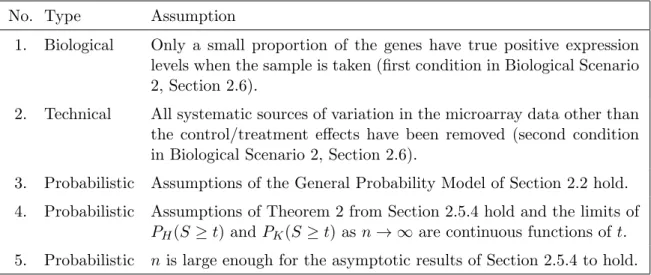
3.1 Biological, technical and probabilistic assumptions. . . 28

3.2 Data 60 hai from tomato plants inoculated with P. infestans. . . 32

3.3 Data 48 hai from Arabidopsis thaliana inoculated with A. tumefaciens. . . . 33

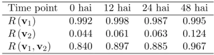
4.1 Inertia ratios for the PI data set. . . 36

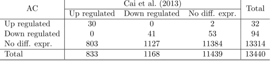
4.2 Comparison with Cai et al. (2013) for PI microarray data set 60 hai. . . 40

4.3 Inertia ratios for the AT data set. . . 41

4.4 Comparison with Ditt et al. (2006) for AT microarray data set 48 hai. . . 44

4.5 Heuristic guidelines for assessing Biological Scenario 2. . . 45

A.1 Down regulated genes in the PI data set 60 hai. . . 51

A.2 Up regulated genes in the PI data set 36 hai. . . 55

A.3 Up regulated genes in the PI data set 60 hai. . . 56

(14)

(15)

List of Figures

2.1 Scanned image of a microarray after hybridization. . . 4

4.1 Inertia ratios R(v2) for the PI microarray data set. . . 36

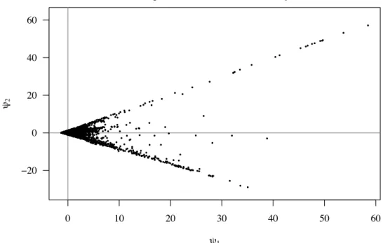
4.2 Artificial components for the PI microarray data set 60 hai. . . 36

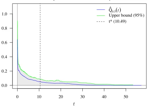
4.3 Estimated pF DR for the PI microarray data set 60 hai. . . 37

4.4 Di↵erentially expressed genes in the PI microarray data set 60 hai. . . 37

4.5 Active vs supplementary time points analysis for the PI microarray data set. 38 4.6 Group conformation through time for the PI microarray data set. . . 39

4.7 Comparison with Cai et al. (2013) for PI microarray data 60 hai. . . 40

4.8 Inertia ratios R(v2) for the AT microarray data set. . . 42

4.9 Artificial components for the AT microarray data set 48 hai. . . 42

4.10 EstimatedpF DR for the AT microarray data set 48 hai. . . 43

4.11 Di↵erentially expressed genes in the AT microarray data set 48 hai. . . 43

4.12 Comparison with Ditt et al. (2006) for AT microarray data 48 hai. . . 44

(16)

(17)

CHAPTER

1

Introduction

Microarray technology has become one of the most important tools in understanding gene expression in biological processes (Yuan & Kendziorski, 2006). Since its development in the 1990s, an enormous amount of data has become available and new statistical methods are needed to cope with its particular nature and to approach genomic problems in a sound statistical manner (Simon et al., 2003). This work focuses on the identification of di↵erentially expressed genes in multiple slide microarray experiments.

As microarrays contain measurements of thousands of gene expression levels across multiple biological conditions, statistical analysis of a microarray experiment necessarily involve data mining or large scale multiple testing procedures. To the date, advances in this regard have either been multivariate but descriptive, or inferential but univariate.

Multivariate approaches developed until now include cluster analysis (Alizadeh et al., 2000; Ross et al., 2000), condition-related directions in the data’s principal

com-ponent space (Ospina & L´opez-Kleine, 2013), permutation validated principal

compo-nents analysis (Landgrebe et al., 2002) and discriminant analysis on principal compocompo-nents (Jombart et al., 2010). However, the statistical significance of the clusters or sets of genes identified as di↵erentially expressed remains an open question –partly because the nature of the data does not easily allow distributional assumptions, and partly because unsupervised classification methods are not guaranteed to identify clusters that actually correspond to di↵erentially expressed genes.

On the other hand, inferential approaches developed so far are based either on para-metric models as ANOVA (Kerr et al., 2000) and Hidden Markov Models (Yuan & Kendziorski, 2006), or in non–parametric multiple testing procedures controlling the

family wise error rate (Sha↵er, 1995; Benjamini & Hochberg, 1995; Benjamini &

Yeku-tieli, 2001; Dudoit et al., 2002) or the false discovery rate (Efron et al., 2001; Tusher

et al., 2001; Storey & Tibshirani, 2001; Storey, 2002; Storey, 2003; Taylor et al., 2005). These methods, however, rely on a gene–by–gene approach in which the multivariate structure of the data is not taken into account.

Thus, multivariate–descriptive and univariate–inferential methods are the two pieces still to be assembled into an integral strategy for the identification of di↵erentially ex-pressed genes in microarray experiments.

(18)

In this work, we present a new strategy that combines a gene–by–gene multiple testing procedure and a multivariate descriptive approach into a multivariate inferential method suitable for microarray data. It is based mainly on the work of Storey & Tibshirani (2001)

for the estimation of thepF DRand on the construction of two artificial components –close

to the data’s principal components, but with an exact interpretation in terms of overall and di↵erential gene expression.

Our method works best under some very common biological and technical assumptions and gives way to a new understanding of gene di↵erential expression. We also provide a methodology to analyse time course microarray experiments and some guidelines for assessing whether the biological and technical assumptions required are likely to hold in a given data set.

We applied our method in two real microarray data sets previously analysed by Cai et al. (2013) and Ditt et al. (2006), respectively. In the first data set, appropriate biological and technical conditions were met and our method proved to be more useful than tradi-tional approaches in that it identified new di↵erentially expressed genes, it o↵ered valuable insights regarding the time course behaviour of the di↵erential expression process, and it avoided wrongly classifying non–expressed genes as di↵erentially expressed. In the second data set, based on the results of our method, we were able to determine that the required biological and technical conditions were not met and thus to conclude that, in such cases, more traditional methods should be preferred.

As a rule, univariate oriented methods identified much more genes as being di↵eren-tially expressed. These discrepancies arise from di↵erences in the biological assumptions that underlie each method and the corresponding implied definitions of di↵erential ex-pression, and, thus, are not indicative of any method’s greater power as a multiple testing procedure. Moreover, when the aim of the study is to perform an intervention upon di↵er-entially expressed genes, our method may prove very valuable as it prevents it from being done upon genes with no expression whatsoever.

As our method constitutes a first multivariate inferential approach to identifying dif-ferentially expressed genes in microarray data, many questions remain open for further investigation. These include statistical assessments of the extent to which our method’s required probabilistic, biological and technical assumptions hold, extensions for when this is not the case, and further applications in biological studies.

This work is constructed as follows. In Chapter 2 we present the theoretical founda-tions that constitute the cornerstones of our methodology, including the basic aspects of microarray experiments, principal components analysis, bootstrap and permutation esti-mation methods, multiple testing procedures and Type I Error measures. In Chapter 3 we present our method for the identification of di↵erentially expressed genes in microarray experiments along with some additional assessments, and introduce two real microarray data sets. In Chapter 4 we apply our method to those data sets and compare our results with previous studies. In Chapter 5 we present our conclusions and outline some open questions and future perspectives.

(19)

CHAPTER

2

Theoretical Framework

In this chapter, we present the theoretical foundations that underlie our methodology. We begin by introducing the basics of gene expression and microarray technology to better understand the nature of microarray data sets, and propose a general probability model for representing this type of data. Then, we introduce the basis of Principal Component Analysis (PCA) and show how to derive a gold–standard for assessing factors or com-ponents that capture desirable features when identifying di↵erentially expressed genes in microarray experiments. Next, we give a brief overview of bootstrap estimation methods and permutation tests. Finally, we reformulate the problem of identifying di↵erentially expressed genes as one of multiple hypothesis testing and present some measures to con-trol Type I Error and false positives in the process. Estimation of those measures is also considered.

As it will be seen, the methods presented in this chapter (included those from Benjamini & Yekutieli, 2001; Tusher et al., 2001; Dudoit et al., 2002; Storey et al., 2004; Dudoit & Van Der Laan, 2008) begin by adopting a gene–by–gene single hypothesis testing approach by means of univariate test statistics and, afterwards, correct for multiple testing. Because the experimental units of a microarray experiment are the replicates (the genes being the variables measured over each replicate), this gene–by–gene approach implies a univariate point of view in which important features of the data remain unaccounted for. In Chapter 3, we propose a method that preserves the multivariate scale of the data by applying the

multiple hypothesis testing procedure for control of thepF DR presented towards the end

of this chapter using a test statistic similar to the principal components in a PCA.

2.1 Background on DNA expression and microarrays

1 _{Gene expression is the process by which di↵erent proteins are synthesized within a cell.}

It consists of the transcription of a gene or a segment of DNA into a complementary

segment (or transcript) of mRNA and its subsequent translation into a protein specific

for that gene. Each DNA segment is a double-stranded polymer composed of four basic molecular units or nucleotides –adenine (A), cytosine (C), guanine (G) and thymine (T)– that follow a unique pairing pattern. When the transcription stage takes place, the two

1_{This section is based on Dudoit et al. (2002) and Simon et al. (2003).} 3

(20)

strands in the DNA segment split and a corresponding segment of mRNA is made by copying one of the strands and replacing the T nucleotide by a uracil (U) base. In the translation stage, this mRNA segment travels to a ribosome in the cytoplasm and directs the synthesis of a molecule of the corresponding protein.

Microarray technology aims at measuring the expression levels of each gene in the genome of a given organism by ways of quantifying the number of mRNA transcripts contained in the cytoplasm of a sample of cells. Because, in theory, there is a one to one correspondence between proteins, mRNA transcripts and its parent genes, and because a single transcript produces a single molecule of its respective protein, mRNA abundance in the transcription stage is assumed to constitute a good measure of gene expression in terms of protein production.

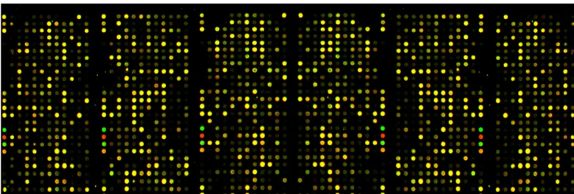
A microarray consists of thousands of genes’ single strands printed on a microscope slide in a high density array (see Figure 2.1). Each spot on the microarray corresponds to a

single gene or expressed sequence tag (EST) and contains many copies of the gene orprobes

printed within. In a microarray experiment, two mRNA samples are reverse transcribed into complementary single strands of DNA (or cDNA) and labeled using fluorescent dyes (usually red and green). The samples are mixed in equal proportions and placed on the array. Then, a competitive hybridization takes place in which transcripts attach themselves to matching probes printed on the microarray. Finally, the microarray is scanned and the red and green intensities are stored in a high resolution image file (see Figure 2.1) from which each gene’s relative amount of mRNA is obtained.

Figure 2.1. Scanned image of a microarray after hybridization.

Taken fromhttp://www.bionivid.com.

Several designs for microarray experiments –in which the number of microarrays and the relations between the treatment/control conditions and the reference/target samples vary– are available (see Simon et al., 2003, Chapter 3). We focus on multiple–slide ex-periments. The basic output of these experiments are the target samples’ intensities in the scanned images after hybridization. If a di↵erent microarray is used for each indi-vidual, a common reference mRNA sample (usually pooled from the control replicates) can be compared against a each individual’s target sample in each microarray. In this case, another output of the experiment consists of the target vs reference samples’ inten-sity ratios. If more than one microarray per individual is available, dye swaps and more elaborate settings are frequently used (Simon et al., 2003).

Because of the technical complexities of microarray experiments –that involve microar-ray printing, mRNA sampling and hybridization, image analysis, etc.–, there are many

(21)

2.2. GENERAL PROBABILITY MODEL FOR MICROARRAY DATA 5 potential sources of systematic variation that may have to be dealt with via quality con-trol and normalization procedures before any further analysis. Rigorous treatment of such procedures, however, is beyond the scope of this work and we will assume here on that normalization procedures, if needed, have been applied as a previous step to our method

for the identification of di↵erentially expressed genes2.

2.2 General probability model for microarray data

We will assume the following probabilistic model holds for microarray data. Denotenthe

number of genes andp=p1+p2the number of replicates, withp1 replicates for treatment

and p2 for control, respectively. Let Xij be the random variable in a general probability

space (⌦,_F, P) that represents the expression level of gene i at replicate j as measured

in microarray experiments, with realization xij and cumulative distribution functionFij.

Then, the column random vectorX_·j represents all the gene expression levels for replicate

j whereas the row random vector X_i· represents the expression levels for gene i across

all replicates; as before, x_·j, F·j, xi· and Fi· denote the realizations and the cumulative

distribution functions of the corresponding random vectors. Finally, define the random

matrix X as (X_·1, . . . , X·p) with realization X = (x·1, . . . , x·p), and joint cumulative

distribution functionF.

In order to provide a general framework for gene expression data, we make the following assumptions:

1. The random column vectors X_·1, . . . , X·p are mutually independent.

2. Let F_·j denote the joint cumulative distribution function of X·j for j = 1, . . . , p.

Then, F_·1 = · · · = F·p1 = FT r and F·p1+1 = · · · = F·p1+p2 = FC, where treatment

and control distributions, FT r and FC, may be di↵erent. This implies Fi1 =· · · =

Fip1 =FiT r and Fi(p1+1)=· · ·=Fip=FiC, for i= 1, . . . , n.

3. The random row vectors X1·, . . . , Xn· are not mutually independent, nor are they

identically distributed.

The first assumption simply states that the replicates are mutually independent, which arises naturally due to experimental conditions. The second imposes identical joint and marginal distributions for treatment replicates and for control replicates separately, but not necessarily equal for all replicates. For this assumption to be plausible, we will assume that the data has been standardized column–wise so that each column has, at least, zero mean and unit variance. The third assumption copes with the fact that di↵erent genes have di↵erent metabolic functions and therefore express themselves in a di↵erent way at di↵erent moments. Also, given that genes usually work in groups (Dudoit & Van Der Laan, 2008), dependence between some of the genes’ expression levels is expected and, so, is included in the model.

Note that this model is very general and that, given the nature of microarray data, further assumptions concerning the dependence structure of the genes or the funcional form of the distributions would be difficult to sustain. In this setup, it will be convenient

to think of the genes as the individuals and the replicates as thevariables of the analysis

(measured over each individual). 2_{See Section 2.6 for more on this subject.}

(22)

2.3 Principal Components Analysis

One of the main objectives of our methodology is to capture and take advantage of the multivariate nature of microarray data throughout the entire analysis. This is not only limited to the correlation structures between genes, already captured by some univariate– approach methods (Benjamini & Hochberg, 1995; Benjamini & Yekutieli, 2001; Tusher et al., 2001; Storey, 2002; Storey & Tibshirani, 2003; Taylor et al., 2005), but also to preserve the relative scale of expression levels among all genes and, so, to be able to an-swer questions like which genes have higher (lower) expression levels, what does ‘higher’ means in terms of the expression levels in a given microarray data set, which di↵erences in expression levels are sufficiently large in this scale, etc. For this, we find that Principal Components Analysis (PCA) is extremely useful. In order to maintain the general prob-ability model for gene expression data of section 2.2 without adding further probabilistic assumptions, we focus on the descriptive stream of standardized PCA and follow Lebart et al. (1995) in its presentation.

2.3.1 PCA mechanics

LetW be an⇥pdata matrix with elementswij representingpmeasurements or variables

for n individuals. One of the aims of PCA is to find the axes or directions in Rp that

capture most of the variability inW. For these directions to capture actual variability and

not variability due to scale and location, the first step is to standardize W column–wise.

LetX ben_⇥p matrix with elements

xij =

wij w¯·j

se(w_·j)

, i= 1, . . . , n, j= 1, . . . , p, (2.1)

where ¯w_·j = n 1Pn_i₌₁wij and se(w·j) = n 1Pn_i₌₁(wij w¯·j)2. Now, every column of

X has zero mean and unit variance. Note that this makes Assumption 2 of the General

Probability Model from Section 2.2 plausible.

Following Lebart et al. (1995), we will capture the variability in X in terms of the

inertia of the rows of X upon each column3_{. For this, let} _d _{be a convenient metric on}

Rp _{represented by the} _p_⇥_p _{symmetric matrix} _D _{with elements} _d

j in the diagonal and

zero otherwise, such that the distance between two vectors x and y in Rp is d(x,y) =

[Pp_j₌₁dj(xj yj)2]1/2. Also, let the n⇥n symmetric matrix Mbe the weights’ matrix,

with elements mi in the diagonal and zero otherwise, mi representing the weight of the

i-th row of X.

BecauseXis standardized column–wise, its center of gravity is the origin and the total

inertia ofX with respect to the origin may be calculated as

In= n X i=1 mid2(xi·,0) = n X i=1 mi p X j=1 djx2ij =tr X0MXD ,

where xi· is the i-th row of X,X0 is X transposed and d2(xi·,0) represents the squared

distance between xi· and the origin under the metric d.

3_{This constitutes the “individuals’ cloud analysis” part of the PCA as explained by Lebart et al. (1995).}

The dual part of the PCA, the “variables’ cloud analysis”, will not be needed farther on and, thus, will be omitted from our presentation. We refer the interested reader to Section 1.2 of Lebart et al. (1995).

(23)

2.3. PRINCIPAL COMPONENTS ANALYSIS 7

Now, let u ₂ _Rp _{be a unitary vector representing any direction in the metric space}

(Rp, d). The coordinates of the orthogonal projections of the n individuals upon the

directionu are

'=XDu, where u0Du= 1, (2.2)

and the inertia projected on u is

In(u) ='0M'=u0DX0MXDu. (2.3)

Note that, 'is centered, but does not necessarily have unit variance.

PCA consists of finding the set of orthogonal unitary vectors in (Rp, d),

{u1, . . . , uk}, k  p, that maximizes the inertia projected upon them. Because

{u1, . . . , uk}is an orthogonal set, the inertia projected on the space generated by them is

justIn(u1, . . . , uk) =In(u1)+· · ·+In(uk). Now, define the firstkPrincipal Components

of X,_{u1, . . . ,uk}, as the solution to the following succesive maximization problems:

Maxu1 : u01DX0MXDu1 s.t. u01Du1= 1, (2.4)

Maxus:s=2, ..., k : u0sDX0MXDus s.t. u0sDur =

⇢

1, s=r

0, s₆=r , r = 1, . . . , s.

Maximization via Lagrange Multipliers yields the solution

X0MXDus= sus, s= 1, . . . , k. (2.5)

Then, it is easy to see that 1, . . . , k and u1, . . . , uk are the first k eigenvalues and

correspondingkeigenvectors ofX0MXD. Also, premultiplying (2.5) byu0_sDand replacing

into (2.3) and (2.4), we getIn(us) = s, s= 1, . . . , k.

Should we have supplementary rows of data in a (n+_⇥_{p) matrix}_W+_{(like individuals}

that where not included in the first analysis or the centers of gravity of groups of indi-viduals), the way to standardize them and project them onto the principal components of the previous PCA is:

x+_ij = w + ij w¯·j se(w_·j) , '+_s =X+Dus, (2.6) fori= 1, . . . , n+, j= 1, . . . , pand s= 1, . . . , k.

Finally, to give a familiar statistical meaning to the previous results, we set D =Ip,

the identity (p⇥p) matrix, and mi = 1/n so that M=n 1In. Then, as the columns in

X have zero mean and unit variance, X0MXD=n 1_X0_X_{is the correlation matrix of} _X

and the total inertia In = tr(n 1X0X) =p. Moreover, s and us, s= 1, . . . , k, are the

eigenvalues and eigenvectors of the correlation matrix of X and the iniertia projected on

any us, s= 1, . . . , k, takes the form of the variance of's from (2.2), that is:

In(us) = s ='0s ✓ 1 nIn ◆ '_s = 1 n n X i=1 '2_is = Var('_s), s= 1, . . . , k.

(24)

2.3.2 A word on interpretation

Because the principal components are the eigenvectors of the standardized data’s

corre-lation matrix, they are entirely determined by X. Moreover, us, s= 1, . . . , k, are also

a solution of (2.4), so the principal components will vary between data sets and their interpretation will be difficult more often than not.

As will be the case in Chapter 3, for detecting di↵erentially expressed genes in a microarray experiment, we need factors or directions that capture two very specific char-acteristics of the data: a gene’s overall expression level and the extent to which it is di↵erentially expressed, both measured with respect to all of the genes’ expression levels. By the nature of PCA, there is no guarantee for a set of microarray data that any of its principal components will capture any of those two features of gene expression.

However, the principal components of the data do provide with a practical gold– standard in terms of captured variability for comparing directions that do refer to a specific set of characteristics (as overall expression levels and di↵erential expression) in a given

microarray data set. For example, letv₂Rpbe an unitary vector in (Rp, d) di↵erent from

the principal components of X. The inertia projected onto v, In(v), can be computed

from (2.3). Define the inertia ratio ofv as

R(v) = In(v)

In(u1)

= In(v)

1

. (2.7)

If a large part of the variability inX relates to direction v,R(v) will be close to one, for

1 is the maximum inertia that can be projected onto any single direction.

Also, if we have access to the same variables measured at di↵erent time points, say,

X(1), . . . , X(L), a practical way to compare the amount of information or variability

cap-tured by a set of orthogonal directions _{v1, . . . , vk} between time points (without

addi-tional probabilistic assumptions) is to compare the ratios

R(l)(v1, . . . , vk) = In(l)(v1, . . . , vk) In(l)_{(u1, . . . ,} _u k) = In (l)_{(v1, . . . ,} _v k) (l) 1 +· · ·+ (l) k , forl= 1, . . . , L. (2.8)

2.4 Bootstrap

In this section we present the basics of the bootstrap estimation method introduced by Efron (1979), following the presentation made by Efron & Tibshirani (1993). The useful-ness of this method in identifying di↵erentially expressed genes will become clear when simulating null distributions and dealing with multiple hypothesis testing farther on. We address bootstrap methods regarding point estimation, confidence intervals and hypoth-esis testing. For simplicity, throughout this section, we use a di↵erent notation from the one in the General Probability Model of Section 2.2.

2.4.1 Bootstrap estimates: One sample case

Suppose we have a data set x = (x1, x2, . . . , xn) that has been generated by random

sampling from a probability distributionF; that is,xis a realization of the random vector

(25)

2.4. BOOTSTRAP 9

Tibshirani (1993)’s notation, we denote this byF _!x. Now suppose there is a parameter

of interest ✓=t(F) and an estimator of✓, say ˆ✓(X) =s(X) for some measurable function

s, with realization or estimate ˆ✓(x) =s(x) and distribution G=F s 1.

Let =t0(G) be a parameter of interest fromG(usual examples are the variance, the

bias or the mean squared error of ˆ✓(X)) to which we may refer to as a “level 2” parameter

of interest (Athreya & Lahiri, 2006). Also, let ˆ = s0(y) be a good estimation of for

any distribution G, should we have access to observations y = (y1, . . . , yn) G. In

theory, we could calculate from F or estimate it from x, but, unless F is known and s

is very simple, there usually is no mathematical formula for this. The bootstrap o↵ers an

alternative way of estimating for which F and Gdo not need to be known.

Let ˜F be the empirical distribution of x, where ˜F is the probability measure that

assigns probability 1/n to each xi in x. In other words, if a random variable X ⇠ F,˜

then P_F˜(X =x) = #{xi =x}/n. The plug-in estimates of ✓ and are ˜✓(x) =t( ˜F) and

˜ = t0( ˜G) = t0( ˜F s 1_{), respectively}4_{. Note that, although computation of ˜}_✓ ₌ _{t( ˜}_F_{) is}

usually straightforward, in general there is no explicit way of calculating ˜ 5.

Given x, define a bootstrap sample ofx or, equivalently, a bootstrap sample from ˜F,

as x⇤ = (xi1, . . . , xin), where (i1, i2, . . . , in) is a random sample of size n drawn with

replacement from _{1,2, . . . , n_}. Note that, by construction, ˜F _! x⇤. Define a bootstrap

replication of ˆ✓(x) as ˆ✓⇤ =s(x⇤). The calculation of the bootstrap estimate of givenx,

ˆ_B_{, is presented in Algorithm 2.4.1.}

Algorithm 2.4.1: Computation of bootstrap estimates in the one sample case.

1. Draw a large number B of independent bootstrap samples from x,x⇤₁, . . . ,x⇤_B.

2. Calculate B bootstrap replications of ˆ✓(x), ˆ✓⇤₁, . . . , ✓ˆ⇤_B, from the bootstrap

sam-ples in the previous step.

3. Estimate as ˆB =s0(ˆ✓⇤1, . . . ,✓ˆB⇤).

When can be expressed as the expected value of a function f of ˆ✓(X) and F (like

the bias EF(ˆ✓ ✓), or the distribution functionEF(I{✓ˆx}) whereI{·}is the indicator

function), step 3 in Algorithm 2.4.1 can be reformulated as

30. Estimate as ˆB =B 1PBb=1f(ˆ✓b⇤).

In such case (Hall, 1992, p. 288), ˆB is an unbiased consistent estimator of ˜, given

x 6_{. That is:}

E_F˜( ˆB) = ˜ and lim

B!1

ˆ

B = ˜,

where the randomness in ˆB given x comes from the random sampling from x. In other

words, the bootstrap estimate ˆB is itself an estimate of ˜, whose accuracy increases

with B. Also, note that in the special case = t0(G) = G, the bootstrap estimate of

4_{It can be proven that ˜}_F_{is a sufficient statistic for}_F _{(Efron & Tibshirani, 1993, p.32) and that ˜}_✓_{and ˜}

are consistent estimators for✓and (Bickel & Doksum, 2001, p. 302). In this sense, the plug-in estimate t( ˜F) is a very good choice for estimatingt(F) if n is large and there is no parametrical assumptions or additional information aboutF other than the datax.

5_{For example, for} _X

⇠ F, estimating E(X) with the sample mean, if = V ar( ¯X), we know that =V ar(X)/n, and ˜ = 1

n

Pn i=1

(xi x¯)2

n . This may be very difficult forsother than the mean.

(26)

the distribution of ˆ✓ given x becomes the empirical distribution of the bootstrap sample ˆ

✓₁⇤, . . . , ✓ˆ⇤_B, ˜GB.

Summarizing, for large B, the bootstrap estimate ˆB is a good approximation of the

plug-in estimate ˜, which, in turn, is a very good estimate of , when no information is

available about F other than the samplex. Note, however, that, even as B ! 1, there

remains uncertainty in ˆB as we are still estimatingF by ˜F and limB!1 ˆB remains the

plug-in estimate of .

2.4.2 Bootstrap confidence intervals

There are multiple ways of computing approximate confidence intervals for a parameter

of interest ✓ using bootstrap methods7. Here, we briefly present two such methods and

some of their properties.

2.4.2.1 Percentile intervals

In normal theory, the bounds of the usual (1 ↵) confidence interval for the mean, ¯x±

z₁ _↵_/₂p

n, are also estimates of the↵/2 and 1 ↵/2 percentiles of ¯X’s distribution. This

property arises from the facts that ¯Xis an unbiased estimator ofµ, that Var( ¯X) is known

and constant for all values of µ, and that pn( ¯X µ)/ is a pivotal statistic (i.e. its

distribution does not depend on unknown parameters). The same principle can be applied to bootstrap estimates as follows.

Under the previous assumptions of unbiasedness and constant variance for ˆ✓ with

respect to✓, a (1 ↵) confidence interval for✓would be [G 1(↵/2), G 1(1 ↵/2)], where

G 1(↵) is the↵percentile of ˆ✓’s distribution. Gbeing unknown, one can approximate such

interval by ways of the bootstrap estimate ofG. Then, forBlarge enough, an approximate

(1 ↵) confidence interval for✓ can be computed as

[✓lo,✓up] =

h

ˆ

✓⇤(B⇥↵/2),✓ˆ⇤(B⇥(1 ↵/2))i (2.9)

where ˆ✓⇤(B⇥↵)denotes the↵percentile of the bootstrap replications ˆ✓⇤(1), . . . , ✓ˆ⇤(B). Note

that ˆ✓⇤(B⇥↵) is the actual ↵ percentile of ˜GB and, by means of the plugin principle, it is

itself an estimate of the ↵ percentile of ˆ✓’s distribution G.

A practical advantage of the percentile interval in (2.9) is that it is

transformation-respecting: ifmis a monotone function defined in the parameter space (Efron & Tibshirani,

1993, p. 175-177), the percentile interval form(✓) is just [m(✓lo), m(✓up)].

Despite the previous properties, use of the percentile intervals is not justified when ˆ✓

is biased for ✓ or when Var(ˆ✓) depends on the true value of ✓. Moreover, the percentile

interval (2.9) is only first order accurate, that is

P⇣✓ˆ⇤(B⇥↵/2) ✓✓ˆ⇤(B⇥(1 ↵/2))⌘= 1 ↵+O(n 1/2).

These limitations are what motivates the construction of BCa intervals presented in the next section.

7_{For a more theoretical treatment of such intervals and their asymptotic properties, the reader is referred}

(27)

2.4. BOOTSTRAP 11

2.4.2.2 BCa intervals

In these section, we outline the construction of BCa intervals for upper confidence bounds. The extension for lower confidence bounds and two-sided confidence intervals is straight-forward and is therefore omitted.

Construction of BCa intervals for✓(BCa standing for “bias corrected and accelerated”)

is based on the following model (Efron & Tibshirani, 1993, p. 326). Suppose there exists

an increasing functionm such that, for =m(✓) and ˆ =m(ˆ✓),

ˆ

⇠N( z0,1), = ₀[1 +a( 0)] (2.10)

where ₀ denotes the standard error of ˆ when = 0, for some 0. Here, z0 is the

bias of ˆ with respect to and arepresents the rate of change of ˆ’s standard error with

respect to changes in .

If (2.10) holds exactly, an exact upper 1 ↵ confidence bound for is

[1 ↵] = ˆ + ˆ

z0+z1 ↵

1 a(z0+z1 ↵)

,

wherez↵is the↵percentile of a standard normal distribution. LetGdenote the cumulative

distribution function of ˆ✓and recall thatmis increasing; the exact upper 1 ↵confidence

bound for ✓is then

✓[1 ↵] =G 1 ✓  z0+ z0+z1 ↵ 1 a(z0+z1 ↵) ◆ , (2.11)

where is the standard normal cumulative distribution function8_{. Note that the function}

m need not be known and that BCa intervals are also transformation-respecting.

When (2.10) does not hold exactly, the error in the approximation will typically be of

order O(n 1), which implies that BCa intervals constructed as in (2.11) are second order

accurate (Efron & Tibshirani, 1993, p. 325-326), that is,P(✓_✓[1 ↵]) = 1 ↵+O(n 1_).

Moreover, BCa intervals are also second order correct (DiCiccio & Efron, 1996).

In practice, we obtain approximate upper confidence bounds for✓ replacingG,z0 and

aby their estimates ˜G, ˆz0 and ˆa, according to Efron (1987) and Efron & Tibshirani (1993,

Chapters 14 and 22). First, we estimate Gwith ˜G_⇡G˜B, for large B. For z0, note that

if (2.10) holds, then ˆ has the same distribution as + (Z z0), where Z ⇠N(0,1).

Then,

P(ˆ✓_✓) =P( ˆ_ ) =P(Z _z0) = (z0).

Then,z0 = 1[P(ˆ✓✓)] and a bootstrap estimate for z0 is

ˆ z0= 1 #_{✓ˆ_b⇤<✓ˆ_} B ! . (2.12)

(28)

For the constanta, Efron (1987) shows that a good estimate is ˆ a= Pn i=1(ˆ✓jack ✓ˆ(i))3 6hPn_i₌₁(ˆ✓jack ✓ˆ(i))2 i3/2, (2.13)

where ˆ✓₍_i₎ = s(x1, . . . , xi 1, xi+1, . . . , xn) is the i-th jackknife value of ˆ✓ and ˆ✓jack =

n 1Pn_i₌₁✓ˆ(i).

2.4.3 Permutation and bootstrap hypothesis tests: Two sample case

In this section we describe two nonparametric procedures for hypothesis testing in the two sample case. Although here we deal mainly with a single hypothesis being tested, the value of these two methods for detecting di↵erentially expressed genes lies on the fact that they provide a useful way of estimating a test statistic’s null distribution under the

general probability model of section 2.2. The general framework is as follows9.

LetX= (X1, . . . , Xp) a random vector with realization x= (x1, . . . , xp), whose first

p1 components are a random sample from a probability distributionF1, say the treatment

group, and whose last p2 components are a random sample from a (possibly di↵erent)

probability distribution F2, say the control group, where p= p1+p2. Note that X may

represent the behaviour of a single gene (a random row vector) in the general probability

model in Section 2.2. Now, our interest may lie in determining whether F1 = F2 or

whether bothF1 and F2 share a common feature, i.e., t(F1) =t(F2), for some function t.

We concentrate on the former.

Define a test statistic s(X) ₂ R, where s is a measurable function, such that large

values ofs(x) are evidence against the null hypothesisH :F1 =F2, and in favour of some

alternative hypothesisK. Now, for a fixed rejection region [t,1), define the decision rule

t such that

t(x) =

⇢

1, s(x)2[t,1) ! We reject H,

0, s(x)₂/ [t,₁) _! We don’t reject H. (2.14)

The significance level of the test t is defined as ↵t = PH( t(X) = 1) and depends on

the rejection region we choose. Here, PH is the probability measure on (⌦,F) when

H is true. For fixed x, the achieved significance level (ASL) or p–value of the test is

ASL= inft{↵t: t(x) = 1}. As↵tis decreasing int, when↵tis also continuous, theASL

may be computed as

ASL=↵_s₍_x₎=PH s(x)(X) = 1 =PH(s(X) s(x)) = 1 GH(s(x)), (2.15)

whereGH denotess(X)’s cumulative distribution function underH. Note that ASL↵t

iif t(x) = 1 iif s(x) t. SoASL(X) =↵s(X) is, itself, a test statistic. Now the question

arises of how to estimate a test statistic’s null distribution without further parametric assumptions.

(29)

2.4. BOOTSTRAP 13

2.4.3.1 Permutation tests

10_{In permutation tests, we need the order representation of the data. Let}_g_{= (g1, . . . , g}

p)

be a vector consisting ofp1ones andp2twos, such thatgi = 1 ifxibelongs to the treatment

group, and gi = 2 if xi belongs to the control group. If H is true, then X1, . . . , Xp are

exchangeable and the vector g has probability 1/ _pp₁ of taking any of its possible _pp₁

values11.

Now, write s(x) = s(x,g) as a function of both x and g and define a permutation

replication of s(x,g) as s⇤ = s(x,g⇤), where g⇤ is any one of the _pp

1 possible vectors

consisting ofp1 ones andp2 twos, keeping xfixed. In other words, g⇤ is a random sample

of size ptaken without replacement from g.

Under H,s(x,g⇤) is a random variable with _pp

1 possible values, each occurring with

probability 1/ _pp₁ , and with realizations(x,g). We define the permutation distribution of

s⇤,Gperm, as the distribution that assigns probability 1/ _pp₁ to each possible permutation

replication of s(x,g). Then, the permutation ASL is defined as

ASLperm=P(s(x,g⇤) s(x,g)) = #{s(x,g

⇤₎ _s_(x,_g)_}

p p1

, (2.16)

wherex remains fixed and the random element isg⇤.

To relate theASLpermto the test’sASLin (2.15), it can be shown (Efron & Tibshirani,

1993, p. 210) that for any 0<↵ <1,

PH(ASLperm<↵)⇡↵,

where the approximation is due only to the discreteness ofGperm. It follows that for small

values of ↵ (as is usually the case) and relatively large values ofp ( 10), by rejecting H

when ASLperm↵, one (approximately) achieves the desired test’s significance level.

In practice, for large p, ASLperm can be approximated by Monte Carlo Methods as

in Algorithm 2.4.2. Note that this is equivalent to computing the bootstrap estimate in

Algorithm 2.4.1, with f(s(x,g)) = I_{s(x,g⇤) s(x,g)_} in step 30, and taking samples

without replacement (instead of bootstrap samples) in step 1. As with bootstrap estimates, [

ASLperm is unbiased and consistent for ASLperm asB ! 1.

Algorithm 2.4.2: Estimation of the ASLpermin permutation tests.

1. Draw a large number B of independent samplesg⇤₁, . . . , g_B⇤ fromGperm.

2. Compute the corresponding permutation replications of s(x,g), s⇤₁, . . . , s⇤_B,

wheres⇤_b =s(x,g⇤_b), b= 1, . . . , B.

3. EstimateASLperm asASL[perm= #{s⇤b s(x,g)}/B.

10_{We follow closely the presentation of the subject in Chapter 15, Efron & Tibshirani (1993).} 11_{This is the “Permutation Lemma” in (Efron & Tibshirani, 1993, p. 207).}

(30)

2.4.3.2 Bootstrap hypothesis tests

12_{In permutation tests, we estimated} _G

H by Gperm, that is, maintaining x fixed and

varying the group vector g. The approach in bootstrap hypothesis tests is somewhat

di↵erent in that it estimatesGH using the plug-in principle. IfH is true, thenx1, . . . , xp

where generated from a common distribution, say,FH, whose plug-in estimate, ˜FH, assigns

1/(p1+p2) probability to each single element inx. Then, underH and keepinggfixed, we

can compute a bootstrap version of the test’sASLusing the plug-in estimate ofs(X,g)’s

cumulative distribution function ˜GH as follows:

ASLboot =PH(s(x⇤,g) s(x,g)) = 1 G˜H(s(x,g)), (2.17)

where x and g are fixed and x⇤ F˜H is a bootstrap sample of x. Here, ASLboot is the

plug-in estimate of the test’s ASLin (2.15).

In practice, we estimate ASLboot with Monte Carlo methods as shown in Algorithm

2.4.3. Once again, ASL[boot is unbiased and consistent for ASLboot as B ! 1, and

consistent for ASLasp_{! 1}and B _{! 1}. It follows that for large values ofp andB, by

rejectingHwhenASLboot↵one (approximately) achieves the desired test’s significance

level.

Algorithm 2.4.3: Estimation of the ASLboot in bootstrap tests.

1. Draw a large number B of independent bootstrap samples fromx,x⇤₁, . . . , x⇤_B.

2. Compute the corresponding bootstrap replications of s(x,g), s⇤₁, . . . , s⇤_B, where

s⇤_b =s(x⇤_b,g), b= 1, . . . , B.

3. EstimateASLboot asASL[boot = #{s⇤_b s(x,g)}/B.

2.4.3.3 Selection of the test statistic

The choice of the test statistic to be used in the previous hypothesis tests depends mainly

on the test’s alternative hypothesisK. If we keep the general hypothesis K:F16=F2, the

power of a given test will increase if the two distributions di↵er in some feature that the

test statistic captures well. For instance, if the true distributions F1 and F2 di↵er only in

their expected value and s(x) = ¯x1 x¯2, the test will have good power of detecting the

alternative. However, ifF1andF2have equal means but unequal variances, the probability

of detectingK using s(x) would be very low (Efron & Tibshirani, 1993, Chapter 15).

For the detection of di↵erentially expressed genes in microarray experiments, one is usually more interested in detecting di↵erences in mean expression levels between treat-ment and control, than in detecting di↵erences in variances or in other functionals of the distributions (Dudoit & Van Der Laan, 2008). We then want a test statistic that captures

di↵erences in the mean expression levels so that ifH is rejected, we know (up to a certain

significance level) that gene’s expression levels following F1 and F2 di↵er at least in their

expected values. Such considerations will be addressed in Chapter 3.

(31)

2.5. MULTIPLE HYPOTHESIS TESTING 15

2.5 Multiple hypothesis testing

When identifying di↵erentially expressed genes in microarray data, one necessarily en-counters simultaneous multiple hypothesis tests: the null hypotheses being those of no di↵erential expression for each one of the thousands of genes under study. Generalizations of the single hypothesis test paradigm have become necessary and di↵erent approaches have been taken in this regard.

In this section, we present two such approaches13: one controlling the family–wise

error rate (FWER), the other based on the false discovery rate (FDR). We discuss the advantages and limitations of each in the context of genetic di↵erential expression. In what follows, we return to the notations and assumptions of the general probability model from Section 2.2.

2.5.1 Some definitions

Lets assume we want to test if a single gene, say genei, is di↵erentially expressed between

treatment and control conditions. Now the null hypothesis would be that of no di↵erential

expression and we can express it as Hi : FiT r = FiC versus an alternative hypothesis

Ki :µiT r6=µiC, where di↵erences in treatment and control expected values are supposed

to imply di↵erential expression14.

Let s(Xi·) be a statistic with realization s(xi·) and cumulative distribution function

Gi, for which large values imply strong evidence againstHi and in favour of Ki. Also, let

t be a decision rule such that

t(xi·) = ⇢

1, s(xi·)2[t,1) ! We rejectHi,

0, s(x_i·)₂/[t,₁) _! We don’t reject Hi. (2.18)

As usual, a Type I Error consists in rejecting Hi when it is true, and a Type II Error

consists in not rejectingHi whenKi is true. Finally, the significance of the test using tis

↵t=P(“Type I Error”) =PHi(s(Xi·) t) = 1 GiHi(t),

wherePHi and GiHi refer to the probability measure in (⌦,F) and the cumulative

distri-bution function of s(X_i·) whenHi is true. In the single hypothesis paradigm, one sets a

desired significance level↵⇤ and chooses tso that ↵t↵⇤.

When detecting di↵erentially expressed genes, we deal with testing H1, . . . , Hn

si-multaneously. Let _G = _{1, . . . , n_} be the set of genes and _H = _{i ₂ _G : Hi is true},

with cardinality n0, be the set of genes for which the null hypothesis is true, i.e., the

set of non di↵erentially expressed genes. Also, for fixed t and rejection region [t,₁), let

Rt = {i2 G :s(Xi·) t}, with cardinality R(t) = R, be the set of genes for which the

null hypothesis is rejected, and let Vt ={i 2G :s(Xi·) t, Hi is true} =Rt\H, with

cardinality V(t) =V, be the set of false positives, that is, the set of genes for which the

null hypothesis is rejected despite being true. Note that R and V are random variables

with realizations r = #{i 2 G : s(xi·) t} and v = #{i 2 G : s(xi·) t, Hi is true},

13_{For a recount of other approaches to multiple hypothesis testing and a thorough theoretical treatment}

see Dudoit & Van Der Laan (2008).

(32)

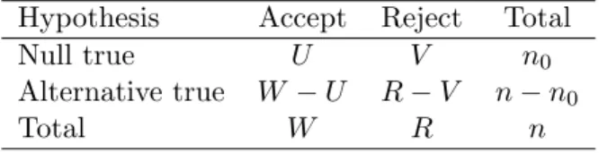
respectively. The possible outcomes of testingH1, . . . , Hnfor fixedtare depicted in Table

2.1. Here, W =n R and U =n0 V.

Table 2.1. Possible outcomes when testingnhypothesis simultaneously.

Hypothesis Accept Reject Total

Null true U V n0

Alternative true W U R V n n0

Total W R n

Adapted from Storey (2002).

Now, the ideal (though generally unattainable) outcome in multiple hypothesis tests

is W _⌘ U and V _⌘ 0, so that all true alternative hypothesis are detected (no Type II

Errors) and no true null hypothesis are rejected (no Type I Errors). When detecting di↵erentially expressed genes, one is more concerned with false positives, hence priority is given to control of Type I Errors. Type II Error reduction may then be achieved by a judicious choice of the test statistic (Efron & Tibshirani, 1993, p. 211).

2.5.1.1 Family-Wise Error Rate

The family-wise error rate (F W ER) is the most stringent measure for controlling Type I Errors in multiple hypothesis tests. It is defined as (Dudoit et al., 2002):

F W ER=P(“At least one Type I Error”) =P(V 1). (2.19)

Most methods that controlF W ER when detecting di↵erentially expressed genes test

for Hi : E(X1) = E(X2) versus Ki : E(X1) 6= E(X2), where X1 ⇠ F1 and X2 ⇠ F2,

and use Welch t-statistics and their p–values to derive ‘adjusted p–values’ as their test statistics (Dudoit et al., 2002). The best known (though most stringent) of such methods is the Bonferroni procedure:

Letpibe the (unadjusted) p–value of thei-th gene’s single hypothesis test using Welch

t-statistic, fori= 1, . . . , n. Define the adjusted p–values ˜pi = min{npi,1} and reject the

null hypothesis for those genes with ˜pi↵⇤. For this procedure, F W ER↵⇤.

There are two downsides with this approach. First, it is too conservative: for very large

n(as is usually the case in microarray experiments) very few, if any, null hypotheses will be

rejected. Second, for small p, one has to know (or make some strong assumptions about)

the Welch t-statistics’ exact joint distributions to compute the adjusted and unadjusted p–values.

To achieve more power, several modifications have been made to the Bonferroni

Pro-cedure, among which is worth mentioning the Westfall & Young (1993)step-down miniP

adjusted p–value and step-down maxT adjusted p–value procedures, for they take into

account the dependence structures among the genes15_.

As to the second downside, Dudoit et al. (2002) extend Westfall & Young (1993) proce-dures by estimating the adjusted and unadjusted p–values with permutation distributions, 15_{When independence among the tests is a reasonable assumption, the reader is referred to the multiple}

(33)

2.5. MULTIPLE HYPOTHESIS TESTING 17 just as permutation tests in Section 2.4.3.1. Dudoit & Van Der Laan (2008) extend this idea by estimating adjusted and unadjusted p–values with bootstrap achieved significance levels as in Section 2.4.3.2.

Despite such improvements, methods that control F W ER remain too conservative

and, loose power as n increases. Additionally, in the context of identifying di↵erentially

expressed genes, control of the F W ER produces a somewhat inappropriate measure of

Type I Error. Given a group of genes identified as di↵erentially expressed, more than the probability of whether any Type I Error was made (F W ER), real interest lies in the number of falsely rejected hypothesis and the proportion of false positives among the group of identified genes (Storey, 2002).

2.5.1.2 False Discovery Rate (FDR)

The previous considerations led to the definition of the false discovery rate (F DR) by Benjamini & Hochberg (1995) as the expected proportion of falsely rejected null

hypoth-esis. For this, define the random variable Q=V /R ifR >0 and Q= 0 otherwise. Then,

theF DR is computed as F DR=E(Q) =E ✓ V R R >0 ◆ P(R >0), (2.20)

where the expectation is taken under the true distributionP instead of the complete null

distributionPH,Hbeing the complete null hypothesisTni=1Hi. Two important properties

arise from this definition:

1. IfH is true (all null hypothesis are true), thenF DR=F W ER. In this case,V =R

soF DR=E(1)P(R >0) =P(V 1) =F W ER.

2. If H is not true (not all null hypothesis are true), then F DR _ F W ER. In this

caseV R soI{V 1} Q. Taking expectations on both sides, we get F W ER=

P(V 1) E(Q) =F DR.

In general, then, F DR _ F W ER so while controlling F W ER amounts to controlling

F DR, the reverse is not true, and, thus, controlling only the F DR results in less strict

procedures and increased power (Benjamini & Hochberg, 1995).

Benjamini & Hochberg (1995) proposed a procedure for controlling the F DR that

consists of fixing a desired F DR level ↵⇤ and determining a suitable rejection region

based on the test statistics’ p–values. More specifically, let p[1] p[2] · · ·p[n] be the

ordered p–values of the test statistics for testing H[1], . . . , H[n], respectively. Now, reject

H_[_i_] for i= 1, . . . , k, where k is the largest integer for which np_[_k_] _k↵⇤. They proved

that if the test statistics are independent, then for the above procedure F DR  ↵⇤ for

every nH = 0,1, . . . , n16. Benjamini & Yekutieli (2001) extended this procedure to the

case when the test statistics present positive regression dependence.

In practice, the statistics’ distributions are unknown, and, thus, the p–values and the

cuto↵khave to be estimated from the data. In this sense, Benjamini & Hochberg (1995)’s

procedure amounts to fixing a desiredF DRlevel and estimating a rejection region

(deter-mined by ˆk) that approximately achieves the desired F DR. Storey & Tibshirani (2001),

(34)

Storey (2002) and Storey & Tibshirani (2003) applied this approach to the identification of di↵erentially expressed genes, estimating the statistics’ distributions and corresponding p–values via permutation and bootstrap distributions and extended it for general statistics other than p–values.

Despite the advantages of Benjamini & Hochberg (1995)’s F DRover theF W ER, the

F DRstill presents some downsides for identifying di↵erentially expressed genes (Storey &

Tibshirani, 2001; Storey, 2002; Storey, 2003). First, ifHis true, every rejected hypothesis

Hi constitutes a Type I Error and one would expect the F DR to be 1 instead of being

equal to the F W ER. Second, being an expectation, controlling the F DR only controls

the ratioV /Rin the long run and the actual ratiov/rmay well be above the desired level

↵⇤. Third, if after performing the test one or more null hypothesis were rejected, that is,

conditioning onR >0, the expected proportion of false positives is only being controlled

at level↵⇤/P(R >0).

2.5.1.3 Positive False Discovery Rate (pFDR)

The positive false discovery rate (pF DR) was introduced by Storey (2002) as a

modifica-tion to Benjamini & Hochberg (1995)’s F DR, motivated by the previous considerations.

It consists of the expected proportion of false positives conditioning onR >0: that is,

pF DR=E ✓ V R R >0 ◆ . (2.21)

Some properties arise from this definition:

1. For t such that17 _P_(s(X

i·) t) >0, i = 1, . . . , n, limn!1P(R > 0) = 1. Then,

for large n, there is little harm in assuming R > 0. Also, limn!1F DR = pF DR

(Storey et al., 2004).

2. If after performing multiple tests no null hypothesis was rejected, then there is no possibility of making a Type I Error and, therefore, the expected proportion of false

positives (conditioning on R > 0 or not) is of no interest and doesn’t have to be

defined for this particular case (Storey, 2003).

3. Note that pF DR F DR, so controlling the pF DR implies control of the F DR.

4. If all null hypothesis are true (V =R), thenpF DR= 1, as desired.

Therefore, pF DR is a more appropriate measure than F DR and F W ER for controlling

Type I Errors in multiple hypothesis testing when nis large (Storey & Tibshirani, 2001;

Storey, 2002; Storey, 2003; Storey & Tibshirani, 2003).

The last property, however, makes it impossible to apply the usual multiple hypothesis

testing paradigm to control thepF DR. Indeed, if H is true, thenpF DR _⌘ 1 and there

is no rejection region such thatpF DR _ ↵⇤ <1 (Storey, 2003). As a result, to perform

multiple tests controlling thepF DR, Storey (2002) proposed to choose a rejection region

and, then, estimate itspF DR; instead of fixing a desiredpF DR and estimating a suitable

rejection region. Storey et al. (2004) proved that in terms of the control for F DR and

pF DR, both types of procedures are asymptotically equivalent.

(35)

As the F DR, thepF DR is also an expectation and, therefore, controlling the pF DR

only controls the ratio V /R in the long run, while the actual realization v/r may exceed

the desired level ↵⇤. Hence, Storey & Tibshirani (2001) recommend to compute upper

confidence bounds for pF DR to asses the possible magnitude of the discrepancy.

Fortu-nately (Storey, 2003, Theorem 4), under some general conditions, the F DR, the pF DR

and the realizedv/max_{r,1_}converge to the same limit as n_{! 1}; so, for large n, these

discrepancies will be small. The remainder of this chapter focuses on estimation and

multiple hypothesis testing when controlling for the pF DR.

2.5.2 Estimation of the pFDR under independence

Storey & Tibshirani (2001) proposed a well behaved finite sample estimator for thepF DR,

given a rejection region [t,₁) and when s(Xi·) are independent and have identical null

distributions. The following Theorem from Storey (2003) is required:

Theorem 1. Suppose n identical hypothesis tests are performed with the statistics Si =

s(X_i·), i = 1, . . . , n, and rejection region [t,₁). Assume that (Si, Hi) are iid random

variables with Si|Hi ⇠(1 Hi)G0+HiG1 for some null distribution G0 and alternative

distribution G1, andHi ⇠Bernoulli(⇡1), for i= 1, . . . , n. Then

pF DR(t) =P(H= 0_|S t), (2.22)

where ⇡0= 1 ⇡1 is the implicit prior probability used in the above posterior probability.

Here, the null hypothesis for gene i being true depends on the random variable Hi

being zero. From (2.22), we obtain

pF DR(t) = ⇡0P(S t|H= 0) P(S t) = ⇡0PH(S t) P(S t) = ⇡0↵t P(S t), (2.23)

where↵tis the significance of a single test using [t,1) as rejection region. For largenand

under some general conditions (see Theorem 2 in Storey & Tibshirani (2001)), (2.23) holds

approximately, even when theHi are not random and the test statisticsSi are dependent

in finite blocks.

The formula (2.23) gives a natural way of estimatingpF DR(t) when the tests statistics

are independent and have the same null distribution. The plug-in estimator ofP(S t)

is R(t)/n.

On the other hand, ↵t = PH(S t) = 1 GH(t), where GH can be approximated

by Gpermor ˜GB via permutation or bootstrap methods from Sections 2.4.3.1 and 2.4.3.2.

More specifically, forBbootstrap or permutation replications (s⇤₁_b, . . . , s⇤_nb), b= 1, . . . , B,

the estimate of↵t is ˆ ↵t= 1 B B X b=1 #i=1,...,n{s⇤_ib t} n = 1 n " 1 B B X b=1 r_b⇤(t) # = EˆH(R(t)) n , wherer⇤_b(t) = #{s⇤_ib t:i= 1, . . . , n}.

Regarding ⇡0, let ↵ = [t↵,1) be the rejection region for which the significance of a

single test PH(S(Xi·) t↵) =↵, and note that { ↵} is a nested set of rejection regions,

(36)

the tests to have a p–value in the interval ( ,1], and, therefore, we also expect n0(1 )

of the test statistics to fall outside . Note also that, for n large enough, ⇡0 = n0/n.

Then, for a well chosen , we can estimate⇡0 as (Storey, 2002):

ˆ ⇡0( ) = #_{Si < t } n(1 ) = n R(t ) n(1 ) = W(t ) n(1 ).

Although identifying exactly for a given may not be straight forward, we can use

t =G_H1(1 ) to estimate t using the bootstrap or permutation estimates of GH, ˜GB

and Gperm.

Storey & Tibshirani (2001) proved that ˆ⇡0( ) is conservatively biased for 0 < <1

and that there is a tradeo↵between bias and variance as varies: increases in produce

larger variances but smaller bias. Storey (2002) proposed a method for finding the value

of that minimizes ˆ⇡0( )’s mean squared error for independent test statistics and Storey

& Tibshirani (2001) generalized it for dependent test statistics. However, to ease the computational burden of our method, we will follow Storey et al. (2004), Taylor et al.

(2005) and Li & Tibshirani (2013) in setting = 0.5.

Replacing into (2.23), we obtain the following estimator for pF DR (Storey, 2002):

ˆ Q (t↵) = ˆ ⇡0↵ˆ ˆ P(S t↵) = ⇡ˆ0EˆH(R(t↵)) R(t↵) . (2.24)

Storey (2002) proved that E( ˆQ (t)) pF DR(t) for all t2R, and⇡0, so ˆQ (t) o↵ers

strong conservative control of thepF DRfor finite samples. Also, if conditions of Theorem

1 hold, ˆQ (t) is a maximum likelihood estimator of

⇡0+⇡1[1 g( )]/(1 )

⇡0

pF DR(t) pF DR, (2.25)

whereg( ) =PK(S t ) 18 (Storey, 2002, Theorem 5). As a result, ˆQ (t) is a consistent

estimator for the left value of (2.25) and is, therefore, consistently conservative for the

pF DR. The steps for computing ˆQ ( ) are depicted in Algorithm 2.5.1, adapted from

Storey & Tibshirani (2001) and Storey (2002).

For small sample sizes, R(t) can be zero with positive probability and (2.24) needs

some modifications to be well defined (Storey & Tibshirani, 2001; Storey, 2002). On

the contrary, if n is large (as it tends to be the case in microarray experiments) under

conditions of Theorem 1 and for non trivial tests19_{, we can safely assume}_P_{(R(t) = 0) = 0.}

18_If_K_{is composite, then}_g_{is formed as an appropriate mixture of alternative distributions (Storey, 2002).} 19_Choosing_t_{so that}_P₍_S _t₎_>_{0. As a result, lim}

(37)

Algorithm 2.5.1: Estimation of thepF DR when testing nhypothesis simultaneously,

for fixed [t,1) and .

1. For large B, compute the bootstrap or permutation replications of

s(x1_·), . . . , s(xn·), obtainings⇤1b, . . . , s⇤nb forb= 1, . . . , B. 2. Compute ˆEH(R(t)) as ˆ EH(R(t)) = 1 B B X b=1 r_b⇤(t), wherer⇤_b(t) = #_{s⇤_ib t:i= 1, . . . , n_}.

3. Set [t ,₁) as rejection region witht as the (1 )-th percentile of the bootstrap

or permutation replications of step 1. Estimate ⇡0 by

ˆ ⇡0( ) = w(t ) n(1 ), wherew(t ) = #{s(x_i·)< t :i= 1, . . . , n}. 4. EstimatepF DR (t) as ˆ Q (t) = ⇡ˆ0EˆH(R(t)) r(t) , wherer(t) = #_{s(xi·) t:i= 1, . . . , n}.

Adapted from Storey & Tibshirani (2001) and Storey (2002).

2.5.3 The q–value

In addition to the pF DR, Storey (2002) proposed theq–value as the analogue of the p–

value when controlling thepF DRin multiple hypothesis testing. For an observed statistic

s(xi·), the q–value is defined as the minimum pF DR that can occur when rejecting all

hypothesis for which s(xi0_·) s(xi·), i0 = 1, . . . , n. More specifically:

q–value(s(xi·)) = inf_t {pF DR(t) :s(xi·) t}. (2.26)

Also, under the conditions of Theorem 1, Storey (2003) shows that

q–value(s(xi·)) =P(H = 0|S s(xi·)),

so the q–value can be interpreted as the posterior probability of making a Type I Error

when testing nhypothesis with rejection region [s(xi·),1).

As ˆQ (t) is not necessarily decreasing in t, we estimate the q–values following

(38)

Algorithm 2.5.2: Estimation of the q–values for testingnhypothesis simultaneously.

1. Let s[1]  s[2]  · · ·  s[n] be the ordered statistics for s[i] = s(x[i]·), for i =

1, . . . , n.

2. Set ˆq(s_[1]) = ˆQ (s_[1]).

3. Set ˆq(s[i]) = min{Qˆ (s[i]),q(sˆ [i 1])}fori= 2, . . . , n.

Adapted from Storey (2002).

2.5.4 A word on dependence

When the test statistics are not independent, the following theorem from Storey & Tib-shirani (2001, Theorem 2) is required:

Theorem 2. Suppose that

Vn(t) #_Hn ! PH(S t) and Rn(t) Vn(t) n #_Hn ! PK(S t),

in probability for some rejection region [t,1) with P(S t)>0. Then

lim

n!1pF DRn(t) =

⇡0PH(S t)

P(S t) ,

where pF DRn(t) is the pF DR of [t,1) resulting from the first n statistics.

If the conditions in Theorem 2 hold, we also have (Storey & Tibshirani, 2001) lim n!1 ˆ Q (t) = ⇡0+⇡1[1 g( )]/(1 ) ⇡0 pF DR(t) pF DR(t),

whereg( ) is a single test’s power when using [t ,₁) as rejection region20. Hence, ˆQ (t)

is still conservatively consistent. Also (Storey, 2003, Theorem 4),

lim n!1 Vn(t) max_{1, Rn(t)} ⇡0PH(S t) P(S t) = 0, almost surely.

Therefore, for largen, thepF DRand the actual (realized) ratiov/max{1, r}are very close

and control of the former amounts to control of the latter. More specifically, ifPH(S t)

and PK(S t) in the conditions of Theorem 2 above are continuous functions oft, then,

for every <1, lim inf n!1 t n ˆ Q (t) pF DR(t)o 0, lim inf n!1 t ⇢ ˆ Q (t) Vn(t) max{1, Rn(t)} 0, (2.27)

with probability 1 (Storey et al., 2004, Theorem 6). This means that, for n large, the

previous results hold for all tsimultaneously. Thus ˆQ (t) is conservatively consistent for

the pF DR and for the realized v/max{1, r}, for all rejection regions of the form [t,1),

20_{Again, if} _K _{is composite, then} _g _{is formed as an appropriate mixture of alternative distributions}

Strategy for multivariate Identification of diferentially expressed genes in microarray data

Strategy for Multivariate Identification of Di

↵

erentially

Expressed Genes in Microarray Data

Juan Pablo Acosta

Universidad Nacional de Colombia

Faculty of Sciences

Statistics Department

Bogot´

a, D.C.

Strategy for Multivariate Identification of Di

↵

erentially

Expressed Genes in Microarray Data

Juan Pablo Acosta

Thesis to qualify for the degree

Advisor

Liliana L´

opez–Kleine, Ph.D.

Research line

Universidad Nacional de Colombia

Faculty of Sciences

Statistics Department

Bogot´

a, D.C.

Acceptation Note

Acknowledgements

Contents

List of Tables

List of Figures

CHAPTER

1

Introduction

CHAPTER

2

Theoretical Framework

2.1

Background on DNA expression and microarrays

2.2

General probability model for microarray data

2.3

Principal Components Analysis

2.4

Bootstrap

2.5

Multiple hypothesis testing