Fast Algorithms for Linear and Kernel SVM+
Wen Li
1Dengxin Dai
1Mingkui Tan
2Dong Xu
3Luc Van Gool
1,4 1Computer Vision Laboratory, ETH Z¨urich, Switzerland
2
School of Computer Science, University of Adelaide, Australia
3
School of Electrical and Information Engineering, University of Sydney, Australia
4VISICS, ESAT/PSI, KU Leuven, Belgium
Abstract
The SVM+ approach has shown excellent performance in visual recognition tasks for exploiting privileged infor-mation in the training data. In this paper, we propose two efficient algorithms for solving the linear and kernel SVM+, respectively. For linear SVM+, we absorb the bias term into the weight vector, and formulate a new optimization problem with simpler constraints in the dual form. Then, we develop an efficient dual coordinate descent algorithm to solve the new optimization problem. For kernel SVM+, we further apply theℓ2-loss, which leads to a simpler
op-timization problem in the dual form with only half of dual variables when compared with the dual form of the original SVM+ method. More interestingly, we show that our new dual problem can be efficiently solved by using the SMO algorithm of the one-class SVM problem. Comprehensive experiments on three datasets clearly demonstrate that our proposed algorithms achieve significant speed-up than the state-of-the-art solvers for linear and kernel SVM+.
1. Introduction
Many computer vision tasks contain privileged informa-tion that only exists in the training data, and not available during the test stage. For example, the training images of many datasets for image recognition are annotated with privileged information such as attributes,object bounding boxes, textual descriptions, depth information. Although the raw test images in the real-world applications are not associated with such information, it has been demonstrated that such information is useful for learning classifiers with better recognition performance [5,11,20,29,32,33,35].
This problem is known as the Learning Using Privi-leged Information (LUPI)problem [32]. Different from the traditional learning paradigm, where the training data and the test data have the same representation, LUPI leverages training data containing additional information that is only available during the training process, not in the testing
pro-cess. Such additional information in the training data is re-ferred to as privileged information or hidden information.
Following the LUPI paradigm, Vapnik and Vashist [32] proposed an SVM-like algorithm called SVM+, in which they replace the slack variables in the standard SVM with a slack function defined in the privileged feature space. Through the slack function, the additional privileged in-formation is used to model the loss function, which guides the hyperplane learning in the main feature space. In trast, the slack variables in the standard SVM are only con-strained to non-negative values, which is often less effective than the slack function in SVM+.
Although SVM+ can be formulated as a quadratic pro-gramming problem in the dual form similarly as the stan-dard SVM, it is still non-trivial to efficiently solve it, be-cause the introduction of the slack function leads to more constraints, and makes the number of dual variables dou-bled. While an SMO-style algorithm was developed in [26], the working set selection method is complicated, and the algorithm is also slow in practice. Moreover, it is unclear how to apply it to linear SVM+ without calculating the ker-nel matrix, which is becoming more crucial, due to rapidly increasing data in real-world applications.
In this paper, we propose two efficient algorithms for solving linear SVM+ and kernel SVM+, respectively. In particular, inspired by linear SVM [16], we augment the feature vector with an additional constant element, and ab-sorb the bias term in the decision function into the weight vector, which leads to a dual form with simpler constraints. The new linear SVM+ formulation can be efficiently solved by using the dual coordinate descent method, in a similar way to linear SVM. For kernel SVM+, we further propose to apply theℓ2-loss, which leads to a simpler optimization
problem in the dual form with only half of dual variables when compared with the original SVM+. More interest-ingly, we show that the resultant dual form is in analogy to one-class SVM, which can thus be efficiently solved us-ing the efficient sequential minimal optimization (SMO) al-gorithm [28] with the existing state-of-the-art SVM solvers
such as LIBSVM [10,1].
We implement our algorithms for linear and kernel SVM+ based on LIBLINEAR [9] and LIBSVM [1], respec-tively. We conduct extensive experiments on three tasks: digit recognition on the MNIST+ dataset [32], scene recog-nition on the Scene-15 dataset [22], and web image retrieval on the NUS-WIDE dataset [4]. The results demonstrate that our proposed algorithms achieve significant speed-up than the state-of-the-art solvers for solving the linear and kernel SVM+ problems.
2. Related Work
Learning Using Privileged Information (LUPI), as a new learning paradigm, was first proposed by Vapnik and Vashist [32], therein with the SVM+ algorithm. After that, many variants of SVM+ have been proposed for solving dif-ferent tasks [24,12, 34,29, 33,23]. In [24], Liang and Cherkassky developed a multi-task learning approach based on SVM+. In [17], a multi-task multi-class extension of SVM+ was proposed. Fouadet al.[12] designed a two-step approach for metric learning, and Xuet al.[34] formulated a convex formulation for metric learning using privileged information based on the information theory metric learning (ITML) method. Sharmanskaet al.[29] proposed the Rank Transfer method for utilizing privileged information, and demonstrated the effectiveness of privileged information in various computer vision tasks. In [23], Liet al. extended SVM+ to the multi-instance learning scenario for image re-trieval and object recognition by learning using web data. In [33], Wanget al.proposed a classifier learning algorithm for utilizing privileged information. In [11], Feyereislet al. extended structure SVM to exploiting privileged informa-tion for object localizainforma-tion.
Vapnik and Vashist also showed that SVM+ has a faster convergence rate than the standard SVM method under cer-tain conditions [32]. A more thorough theoretic study of SVM+ can be found in [27]. In [31], two mechanisms for LUPI are further explained. Lapinet al.[21] also discov-ered the relationship between SVM+ and weighted SVM, while Liet al.[23] discussed the connection of the unsuper-vised domain adaptation method and SVM+.
One closely related work is [26], in which an SMO-style algorithm was developed for the SVM+ problem. However, as the two sets of dual variables introduced for the con-straints related to the main and privileged features in the primal form are tangled together in the constraints of dual problem, it is non-trivial to design the working set selection method for the SMO algorithm, and leads to a complicated algorithm that is less efficient in practice. Moreover, it is also unclear that how to apply the the SMO-style algorithm for solving the linear SVM+ problem without calculating the kernel matrix. In contrast, in this paper, by absorbing the bias term into the weight vector of the SVM+ classifier, we
arrive at an optimization problem with simpler constraints in the dual form. Thus, the conventional dual coordinate descent algorithm can be applied to efficiently solve linear SVM+. Moreover, for the SVM+ form, we further apply the
ℓ2-loss and obtain a smaller dual problem with only a half of
dual variables of the original SVM+ formulation. The new dual form shares a similar formulation with one-class SVM, and thus can be solved by using the SMO algorithm imple-mented in the existing SVM solvers such as LIBSVM [1] without developing any new specific SMO algorithm. We demonstrate that our proposed two algorithms are more ef-ficient than the SMO-style algorithm in [26].
We are also aware that there are some works proposed for solving the tasks in which training and test data contains different information, which are less related to SVM+ [2,3, 5,7,13,14,15,20,30,35].
3. Learning Using Privileged Information
In the following, we denote a vector (resp., matrix) with a lower (resp., upper) case letter in boldface. For example,arepresents a vector, andAa matrix. The transpose of a vector or matrix is denoted by using the superscript′. We use 0n,1n ∈ Rn to represent the column vector with n zeros and ones, respectively. We also simply use0and1
instead of0nand1n, when the dimensionality is obvious. Moreover,a◦b(resp.,A◦B) denotes the element-wise product between two vectors (resp., matrices).
In the Learning Using Privileged Information (LUPI) paradigm [32], the training samples contain additional in-formation that is not available in the test stage. Formally, we represent the training data as{(xi,x˜i, yi)|i= 1, . . . , n}, wherenis the total number of training samples,xi ∈ RD is the main feature vector of the i-th training sample with
D being the feature dimensionality, ˜x ∈ RD˜ is the corre-sponding privileged feature vector withD˜ being its dimen-sion. The goal of LUPI is to learn a decision functionf(x)
for classifying any test samplex∈RDin the main feature space.
In [32], an SVM based approach calledSVM+was pro-posed. Similar to SVM, the decision function in SVM+ is represented as f(x) = w′ϕ(x) +b, where ϕ(·)is a fea-ture mapping induced by the kernel on training data,w is the weight vector, andbis the bias term. The objective of SVM+ can be written as,
min ˜ w,˜b,w,b 1 2 ( ∥w∥2+γ∥w˜∥2)+C n ∑ i=1 ξ( ˜w,˜b, ψ(˜xi)) (1) s.t. yi(w′ϕ(xi) +b)≥1−ξ( ˜w,˜b, ψ(˜xi)), (2) ξ( ˜w,˜b, ψ(˜xi))≥0, (3)
whereξ( ˜w,˜b, ψ(˜xi)) = ˜w′ψ(˜x) + ˜b is the slack function defined in the privileged feature space, ψ(·)is the feature mapping function for the privileged features, andw˜ and˜b
are respectively the weight vector and bias term for the slack function. It can be observed that SVM+ replaces the slack variables in the standard SVM formulation with the slack functionξ( ˜w,˜b, ψ(˜xi)). As a result, the loss occurred by the training samplesxican be regularized by the privileged informationx˜i, therefore the hyperplane of SVM+ classifier can be tuned by using the privileged information during the training process.
Let us introduce two sets of dual valuables{αi|n i=1}and
{ζi|n
i=1}for the constraints in (2) and (3), respectively, and
also denote two vectorsα= [α1, . . . , αn]′ ∈Rnandζ =
[ζ1, . . . , ζn]′∈Rn. We arrive at the dual form of SVM+,
min (ζ,α)∈A 1 2(α◦y) ′K(α◦y)−1′α (4) +1 2γ(α+ζ−C1) ′K˜(α+ζ−C1), whereA={(ζ,α)|y′α= 0,1′(α+ζ−C1) = 0,α ≥ 0,ζ ≥ 0} is the feasible set of(α,ζ),K ∈ Rn×n is the kernel matrix based on the main training features with each element beingKij = ϕ(xi)′ϕ(xj), andK˜ ∈ Rn×n is the kernel matrix based on the privileged features with each el-ement beingK˜ij =ψ(˜xi)′ψ(˜xj). After solving the above problem, the weight vectorswandw˜ can be reconstructed based on the Karush-Kuhn-Tucker (KKT) conditions as,
w = n ∑ i=1 αiyiϕ(xi), (5) ˜ w = 1 γ n ∑ i=1 (αi+ζi−C)ψ(˜xi). (6)
Although the dual problem in (4) is a quadratic pro-gramming problem, solving it with the existing optimiza-tion toolboxes is certainly undesirable for real-world visual recognition tasks. However, it is non-trivial to develop effi-cient algorithm like the SMO algorithm for solving the stan-dard SVM. The main difficulty comes from the constraint
1′(α+ζ−C1) = 0, in which two sets of dual variables are tangled together, which makes the working set selection method become complicated [26].
4. Dual Coordinate Descent Algorithm for
Solving Linear SVM+
In this section, we present the dual coordinate descent method for solving the linear SVM+. In particular, we ab-sorb the bias term into the weight vectorwby appending a constant entry of1to each feature vector,i.e.,x←[x′,1]′, andw ← [w′, b]′ for the main features, andx˜ ← [˜x′,1]′, andw˜ ← [ ˜w′,˜b]′ for privileged information. For ease of presentation, we still usew andx(resp., w˜, ˜x) to repre-sent the weight vector and feature vector for the main (resp., privileged) features.
Now, the objective of linear SVM+ can be reformulated as follows, min ˜ w,w 1 2 ( ∥w∥2+γ∥w˜∥2)+C n ∑ i=1 ˜ w′˜x (7) s.t. yiw′xi≥1−w˜′x˜, ˜ w′x˜i ≥0, and its dual form can be written as,
min (ζ,α)∈A 1 2(α◦y) ′K(α◦y)−1′α (8) + 1 2γ(α+ζ−C1) ′K˜(α+ζ−C1),
where the feasible set becomesA = {(ζ,α)|α ≥0,ζ ≥ 0},K ∈Rn×n is the linear kernel matrix of main features defined asKij = x′ixj, andK˜ ∈ Rn×n is the linear ker-nel matrix of privileged features defined as K˜ij = ˜x′i˜x′j. Compared to the dual form of the original SVM+ formula-tion (4), the objective function remains the same, but we do not have the constraintsy′α = 0,1′(α+ζ−C1) = 0
in (8), after absorbing of the bias terms in (7). The weight vectors w andw˜ can be represented using the dual vari-ables in the same way as in (5) and (6) without using the feature mapping functions (i.e., we can setϕ(xi) =xiand
ψ(˜xi) = ˜xi. Let us define Q = [ K◦(yy′) + 1 γK˜ 1 γK˜ 1 γK˜ 1 γK˜ ] ∈ R2n×2n, β = [α′,ζ′]′ ∈ R2n, e = [(1 + C γK1˜ )′,( C γK1˜ )′]′∈R
2n, the problem in (8) can be rewrit-ten in a more concise form as,
min β 1 2β ′Qβ−e′β (9) s.t. β≥0.
Now we develop a coordinate descent algorithm for the problem in (9) similarly as that for linear SVM [16]. In the dual coordinate descent algorithm, we iteratively update one entry ofβeach time. This process is repeated until the stopping criterion is reached.
In particular, let us denotef(β) =1
2β′Qβ−e′β, and we
propose to update thei-th entry asβi ←βi+d, wheredis a scalar variable that needs to be solved. By definingδ(i)= [0, . . . ,0,1,0, . . . ,0]as the vector with all zeros except the
i-th entry being one, the subproblem for solvingdcan be formulated as
min
d f(β+dδ
(i)) s.t. β+dδ(i)≥0, (10)
which has an analytic solution as follows,
d= max(−βi,−∇i
f(β) Qii
whereQii is the(i, i)-th entry of the matrixQin (9), and ∇if(β)is the gradient off(β)w.r.t.βi.
Now we discuss how to efficiently calculate the right-hand side of (11). The scalar Qii can be pre-computed efficiently, so the major problem is the calculation of ∇if(β). In particular, the gradient off(β) can be writ-ten as∇f(β) =Qβ−e. Then, for any given indexi, the gradient off(β)w.r.t.βican be calculate as,
∇if(β) = (Qβ)i−ei=
2n ∑ j=1
Qijβj−ei, (12)
whereQijis the(i, j)-th element of the matrixQ, andeiis thei-th element of the vectore.
We discuss the detailed calculations in two cases. Let us denote a matrixH=K◦yy′∈Rn×n. For∀i= 1, . . . , n, we have 2n ∑ j=1 Qijβj= n ∑ j=1 Hijαj+ 1 γ n ∑ j=1 ˜ Kijαj+ 1 γ n ∑ j=1 ˜ Kijζj
whereHijis the(i, j)-th element of the matrixH. We also haveei = 1 +Cγ
∑n
j=1K˜ij. By applying the KKT condi-tionsw.r.t.wandw˜ in (5) and (6), the gradient offw.r.t.βi in (12) can be written as,
∇if(β)i =yiw′xi−1 + ˜w′x˜i, ∀1≤i≤n (13) which takesO(D+ ˜D)time complexity, and it can be fur-ther speed-up if the feature vectorsxandx˜are sparse.
Similarly, for∀i=n+ 1, . . . ,2n, we have
2n ∑ j=1 Qijβj = 1 γ n ∑ j=1 ˜ Kijαj+ 1 γ n ∑ j=1 ˜ Kijζj, andei= Cγ ∑n
j=1K˜ij. By using the KKT condition forw˜ in (6), the gradient in (12) can be written as,
∇if(β)i= ˜w′x˜i, ∀n+ 1≤i≤2n, (14) which takes O( ˜D)time complexity only, and can also be further speed-up if the feature vectorx˜is sparse. This com-pletes the calculation of (11).
After solvingd, we update thei-th dual variableβi by using βi ← βi +d. Considering only one dual variable is modified each time, the weight vectors can be updated efficiently at each iteration. Note that we have αi = βi when1 ≤ i ≤n, and ζi−n = βi, whenn+ 1 ≤ i ≤ n. Based on (5) and (6), the updating rules forwandw˜ can be written as
w ← w+dyixi, if1≤i≤n (15)
˜
w ← w˜ + 1
γdx˜i, if1≤i≤2n (16)
Algorithm 1Dual coordinate descent algorithm for solving the linear SVM+ problem in (7)
Input: {(xi,x˜i, yi)|ni=1},C, andγ.
1: Initializew=0, andw˜ =−Cγ ∑ni=1x˜i.
2: SetQii = x′ixi for1 ≤ i ≤ n, andQii = ˜x′ix˜i for
n+ 1≤i≤2n. 3: repeat
4: Randomly pick an indexi. 5: if1≤i≤nthen
6: Calculate∇if(β)using (13). 7: else
8: Calculate∇if(β)using (14).
9: end if
10: Calculatedusing (11) based onQiiand∇if(β). 11: if1≤i≤nthen
12: Updatewusing (15).
13: end if
14: Updatew˜ using (16).
15: untilThe convergence criterion is reached.
Output: Weight vectorswandw˜.
We summarize our dual coordinate descent algorithm for solving linear SVM+ in Algorithm1. We first initialize the weight vectors asw=0D, andw˜ =−Cγ ∑ni=1x˜i(i.e., the solution ofwandw˜ whenα=0andζ=0). Then, each time, we randomly pick up an indexi, and solved(i.e., the change ofβi) using (11). In particular, when1 ≤ i ≤ n, we calculate the gradient∇if(β)using (13), and update the weight vectorswandw˜ using (15) and (16), respectively; whenn+ 1 ≤ i ≤2n, we calculate the gradient∇if(β)
using (14) and update the weight vectorw˜ only using (16). The above process is repeated until the objective converges. Actually, the problem in (9) can be treated as a special form of the linear SVM problem discussed in [16], so the conver-gence of our algorithm follows that of the dual coordinate descent algorithm for linear SVM. We implement our algo-rithm based on the LIBLINEAR software [9].
5. SMO Algorithm for Solving Kernel SVM+
In this section, we develop an efficient algorithm for solving kernel SVM+ based on the ρ-SVM formulation. Similar to linear SVM+, we also augment the feature vec-tor in the nonlinear feature space, so we can absorb the bias term into the weight vector,i.e.,ϕ(xi) ←[ϕ(xi)′,1]′ andw ← [w′, b]′ for the main features (resp.,ψ(˜xi) ←[ψ(˜xi)′,1]′ andw˜ ←[ ˜w′,˜b]′for the privileged features)1. For ease of presentation, we still use ϕ(xi) andw to
de-1Usually we do not know the explicit form ofϕ(·), but the inner
prod-uct of the augmented features can be simply calculated by adding one,i.e., ϕ(xi)′ϕ(xj)←ϕ(xi)′ϕ(xj) + 1, so the kernel matrix based on the aug-mented features can be calculated byK←K+11′. The same approach can be applied to the privileged features.
note the nonlinear feature and weight vector for the main features (resp.,ψ(˜xi)andw˜ for privileged features) below. Specifically, after using the augmented features, the de-cision function can be represented asf(x) =w′ϕ(x). We use the squared hinge loss forρ-SVM, which leads to theℓ2
lossρ-SVM formulation as follows,
min w,b,ρ 1 2∥w∥ 2+1 2C n ∑ i=1 ξi2−ρ (17) s.t. yi(w′ϕ(xi))≥ρ−ξi.
By replacing each slack variableξiwith the slack func-tionξ(˜xi) = ˜w′ψ(˜xi), we arrive at the primal form ofℓ2
-SVM+ as follows, min ˜ w,w,ρ 1 2 ( ∥w∥2+γ∥w˜∥2)+1 2C n ∑ i=1 ( ˜w′ψ(˜xi)) 2 −ρ s.t. yi(w′ϕ(xi))≥ρ−w˜′ψ(˜xi). (18) Now we derive the dual form of ourℓ2-SVM+
formula-tion in (18). By introducing dual variablesα1, . . . , αn for the constraints in (18), we write its Lagrangian as follows,
L= 1 2 ( ∥w∥2+γ∥w˜∥2)+1 2C n ∑ i=1 ( ˜w′ψ(˜xi)) 2 −ρ (19) − n ∑ i=1 αi(yi(w′ϕ(xi))−ρ+ ˜w′ψ(˜xi)),
Let us denote a vector α = [α1, . . . , αn]′. By setting the derivatives of (19)w.r.t.to the primal variablesw,w˜, ρ
to zeros, we obtain the constraintα′1 = 1as well as two KKT conditions forwandw˜ as,
w = n ∑ i=1 αiyiϕ(xi), (20) ˜ w = n ∑ i=1 αi(γI+CPP′)− 1 ψ(˜xi), (21)
whereP= [ψ(˜x1), . . . , ψ(˜xn)]is the data matrix of privi-leged features in the nonlinear feature space.
Substituting the two equations in (20) and (21) into the Lagrangian in (19), we arrive at the dual form of (18),
min α 1 2α ′(H+G)α (22) s.t. 1′α= 1, α≥0, whereG = P′(γI+CPP′)−1P,H = K◦(yy′), and
K is the kernel matrix of augmented main features with
Kij = ϕ(xi)′ϕ(xj)being its (i, j)-th element. Based on the equation(γI+CPP′)−1P=P(γI+CP′P)−1, we have G = P′P(γI+CP′P)−1 = ˜K ( γI+CK˜ )−1 ,
Algorithm 2Algorithm for solving theℓ2-SVM+ problem
in (18) Input: K,K˜ ∈Rn×n,C, andγ. 1: CalculateG=C1I−C1 ( I+CγK˜ )−1 . 2: SetQ=H+G, andν = 1/n.
3: Obtainαby solving the problem in (23) with the one-class SVM solver in LIBSVM.
Output: Dual variable vectorα.
whereK˜ is the kernel matrix of augmented privileged fea-tures with K˜ij = ψ(xi)′ψ(xj)being its(i, j)-th element. By further applying the Woodbury Identity, we obtainG=
1 CI− 1 C ( I+CγK˜ )−1 .
Note the problem in (22) is a quadratic programming problem with the number of dual variables beingn, which is only half number of variables in the dual form of the orig-inal SVM+ method in (4). Moreover, the constraints in (22) are also simpler, so it can be solved by using the efficient SMO algorithm. Actually, the problem in (22) shares a sim-ilar form with one-class SVM in the LIBSVM software [1]. In particular, we write the dual form of one-class SVM as follows (Eqn. (8) in [1]), min α 1 2α ′Qα (23) s.t. 1′α=νn, 0≤α≤1,
whereQis the kernel matrix in one-class SVM,νis a pre-defined parameter,nis total the number of training samples. Note the constraints α ≥ 0and1′α = 1in (22) imply
0≤α≤1. By settingQ= (H+G)andν= n1, the dual problem ofℓ2-SVM+ in (22) can be converted to the
opti-mization problem in (23). Therefore, we ignore the details of the SMO algorithm here, and employ the SMO imple-mentation in LIBSVM to solve ourℓ2-SVM+ problem.
The detailed algorithm for solvingℓ2-SVM+ is described
in Algorithm2. We first calculate the matrix Gusing the kernel matrix of privileged features. Then we call the one-SVM solver in LIBone-SVM to obtain the dual variable vector
α. Finally, the decision function can be written asf(x) =
∑n
i=1αiyiϕ(xi)′ϕ(x), wherexis the test sample, andϕ(·)
is the augmented nonlinear feature vector.
Although in our algorithm a matrix inverse operator is involved when calculating the matrixG, the size ofGis onlyn×n, and the subsequent QP problem is also only withndual variables. With the excellent implementation of matrix inverse function such as that in MATLAB, and the SMO implementation in LIBSVM, our algorithm is much faster than the existing SVM+ solver [26] in practice.
Moreover, in some scenarios such as multi-instance learning using privileged information [25], it often needs to
iteratively solve the SVM+ problem. In this case, after cal-culating the matrix inverse, we only need to iteratively solve the one-class SVM, which is much more efficient than the traditional method which needs to iteratively optimize a QP problem for solving the SVM+ problem (see Section6.2).
6. Experiments
In this section, we evaluate the efficiency of our proposed two algorithms for linear and kernel SVM+, and compare them with the existing SVM+ solvers for the image clas-sification and web image retrieval tasks. Considering we solve two variants of SVM+ instead of the original SVM+ formulation, we also report the classification/retrieval per-formance for comparisons.
6.1. Image Classification
We conduct the experiments for two image recognition tasks: digit recognition and scene recognition.
Datasets: In the digit classification task, Vapnik and Vashist [32] have shown that the additional textual descrip-tions in training data are helpful for learning a better clas-sifier. We employ the benchmark MNIST+ dataset used in [32,26] for classifying the images as two digits “5” and “8”. The dataset is constructed by using a subset of the MNIST dataset containing the images of the digits “5” and “8”. It is split into a training set of100images (50images with digit “5”, and 50 images with digit “8”), a validation set of4,002
images, and a test set of1,866images. All the images are resized into 10×10 pixels, and the 100-d vector of raw pixels is used as the main feature vector for each image. Each training image is additionally supplied with a poetic description (see [32] for the examples), which is converted into a21-d textual feature vector, and used as the privileged information in SVM+.
For the scene recognition task, we employ the Scene-15 dataset[22], which contains4,485 images of15different scenes. We split the data into three sets: 300images as the training set, 40% images as the test set, and the rest as the validation set. We downsample all the images by factor3, because small images are preferred in real-world applica-tions for saving the storage of visual data at test time. The CNN features [19] are extracted with the CAFFE frame-work [18], which has shown good performance in various visual recognition tasks. During training, the CNN fea-tures extracted from the original images are treated as privi-leged information, and the CNN features extracted from the downsampled images as the main features. The experimen-tal setting is inspired by [6], where high-resolution images yield superior performance than low-resolution images for standard vision tasks. PCA is applied on two types of fea-tures to obtain 100-d compact representations.
Baselines: In our experiments, we consider two settings, the linear case and the nonlinear case. In the linear case,
there is no solver specifically designed for linear SVM+. So we mainly compare our method with the following two baselines,
• LIBLINEAR: The standard linear SVM without us-ing privileged information implemented in LIBLIN-EAR [9]. We include it as a baseline for investigating the effectiveness of our linear SVM+ formulation. • gSMO: The SMO-style algorithm for solving SVM+
in the dual form, which is proposed in [26]. We use the released C++ implementation from the authors. Note that the gSMO method was designed for solving ker-nel SVM+, but it can still take the feature vectors as the input. So we also include it as a baseline for the linear case. For the nonlinear case, the Gaussian kernel is used for all the methods, in which the bandwidth parameter is set as the mean of distances between all training samples by default. Besides the aforementioned gSMO method, we also com-pare our ℓ2-SVM+ method with the existing
state-of-the-art solvers of SVM+, and also include the standard SVM solved by LIBSVM as a baseline for investigating the effec-tiveness of SVM+.
• SVM: The standard SVM without using privileged in-formation, whihc is solved by using LIBSVM [9]. We include it as a baseline for investigating the effective-ness of ourℓ2-loss SVM+ formulation.
• CVX-SVM+: An implementation based on the CVX optimization toolbox provided in [24]. It directly solves the quadratic programming problem in (4) us-ing the QP solver in CVX.
• MAT-SVM+: We additionally include the QP solver implemented in MATLAB R2014b as a baseline, and employ it to solve the QP problem in (4).
For all methods, the tradeoff parameters are determined based on the validation set. One-vs-all strategy is used on the Scene-15 dataset, which contains 15 classes. The classi-fication accuracy on the test set is reported for performance evaluation. The training time of all methods is measured on a workstation with Intel i7-3770K [email protected].
6.1.1 Experiments on Linear SVM+
Experimental results: The classification accuracies and training time of all methods on two datasets are summa-rized in Table1. In terms of the classification accuracy, we observe that both our linear SVM+ algorithm and gSMO achieve better results than the baseline linear SVM method, which demonstrates the effectiveness of exploiting the po-etic description as privileged information for improving the image based digit recognition task. Our method achieves slight better results than the gSMO method, possibly be-cause we use a new variant of SVM+, and our dual coordi-nate descent algorithm guarantees the optimal solution.
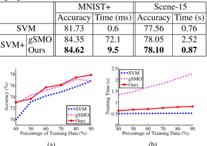
Table 1. Accuracies (%) and training time of all methods on the MNIST+ and Scene-15 datasets in linear case. Our results are highlighted in boldface.
MNIST+ Scene-15 Accuracy Time (ms) Accuracy Time (s) SVM 81.73 0.6 77.56 0.76 SVM+ gSMO 84.35 72.1 78.05 2.52 Ours 84.62 9.5 78.10 0.87 40 50 60 70 80 90 70 72 74 76 78
Percentage of Training Data (%)
Accuracy (%) SVM gSMO Ours (a) 40 50 60 70 80 90 0 0.5 1 1.5 2 2.5
Percentage of Training Data (%)
Training Time (s)
SVM gSMO Ours
(b)
Figure 1. The accuracies (Figure (a)) and the training time (Fig-ure (b)) of different methods for solving linear SVM+ when using different number of training samples on the Scene-15 dataset.
In terms of the training time, both SVM+ algorithms are slower than the baseline linear SVM, because that more complicated objective functions are used to incorporate privileged information. Our new dual coordinate descent al-gorithm for linear SVM+ is much faster than gSMO, which generally takes only a bit more training time than the linear SVM as shown in Table1.
Results using different number of training samples:We further take the Scene-15 dataset to investigate the accura-cies and efficiency of different methodsw.r.t.different num-ber of training samples. Similarly as in [32,26], we ran-domly sample 40%,50%,60%,70%,80% and90% train-ing samples for learntrain-ing SVM and SVM+ classifiers. The experiments are repeated for10times, and we plot the av-erage accuracies and training time of different methods in Figure 1. While the accuracies of all methods become higher when the number of training data increases, our lin-ear SVM+ algorithm consistently outperforms the linlin-ear SVM method, and generally achieves slight better perfor-mance than the gSMO method. In term of the training time, it can be observed that the training time of our method in-creases linearlyw.r.t.the number of training samples, and is several times faster than the baseline gSMO method.
Convergence: As mentioned in Section 4, our algorithm can be treated as a special form of the linear SVM discussed in [16]. So it shares the similar convergence property as the dual coordinate descent algorithm for linear SVM. To verify the convergence of our algorithm, in Figure2, we take the MNIST+ dataset as an example to plot the objective values of our algorithm when the number of iterations2increases. It can be observed that our algorithm converges well. The
2Similarly as in LIBLINEAR, one iteration refers to that we pass all
training samples once.
100 101 102 103 −2 0 2 4 6x 10 4 Number of Iterations Objective Value
Figure 2. The objective of our coordinate descent algorithm for linear SVM+ on MNIST+ dataset.
objective value decreases very fast within the first ten itera-tions, and continues to decrease as the number of iterations increases.
6.1.2 Experiments on Kernel SVM+
Experimental results: We report the classification accu-racies and training time of all methods on two datasets when using the Gaussian kernel in Table 2. On the MNIST+ dataset, we observe that the SVM+ algorithms again achieve better results than the baseline SVM algo-rithm, due to the utilizing of poetic descriptions as priv-ileged information. However, on the Scene-15 dataset, gSMO and CVX-SVM+ are worse than the standard SVM method. Ourℓ2-SVM+ algorithm achieves better result than
the baseline algorithms, showing our new formulation for kernel SVM+ is effective for the scene classification prob-lem on this dataset.
In terms of the training time, we observer that our newly proposed algorithm is the most efficient one among all SVM+ algorithms, and generally achieves order-of-magnitude speedup over the second fastest algorithm (MAT-SVM+ on the MNIST+ dataset, and gSMO on the Scene-15 dataset). The results demonstrate the efficiency of our new reformulation of kernel SVM+. With the reformulation, we convert it as a one-class SVM problem, and take advantage of the existing state-of-the-art SMO implementation in LIB-SVM to solve it.
Results using different number of training samples:
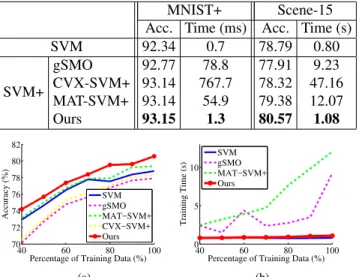
Similarly as for the linear case, in Figure 3, we take the Scene-15 dataset to plot the classification accuracies and training time of different methods by using different per-centages of training data. The CVX-SVM+ method is not included when reporting the training time for better visu-alization. We observe that ourℓ2-SVM+ algorithm
outper-forms other SVM+ algorithms in terms of both classifica-tion accuracy and efficiency when varying the number of training samples.
6.2. Web Image Retrieval
In this subsection, we demonstrate the advantage of our ℓ2-SVM+ algorithm for solving the multiple instance
Table 2. Accuracies (%) and training time of all methods on the MNIST+ and Scene-15 dataset using the Gaussian kernel. Our results are highlighted in boldface.
MNIST+ Scene-15 Acc. Time (ms) Acc. Time (s) SVM 92.34 0.7 78.79 0.80 SVM+ gSMO 92.77 78.8 77.91 9.23 CVX-SVM+ 93.14 767.7 78.32 47.16 MAT-SVM+ 93.14 54.9 79.38 12.07 Ours 93.15 1.3 80.57 1.08 40 60 80 100 70 72 74 76 78 80 82
Percentage of Training Data (%)
Accuracy (%) SVM gSMO MAT−SVM+ CVX−SVM+ Ours (a) 40 60 80 100 0 5 10
Percentage of Training Data (%)
Training Time (s) SVM gSMO MAT−SVM+ Ours (b)
Figure 3. The accuracies (Figure (a)) and training time (Figure (b)) of different methods for solving kernel SVM+ when using differ-ent number of training samples on the Scene-15 dataset.
learning using privileged information problem. We em-ploy the mi-SVM-PI algorithm proposed in [25] to eval-uate different SVM+ solvers. The mi-SVM-PI algorithm needs to iteratively solves the SVM+ problem, and simul-taneously infer the labels for training samples under MIL constraints. We compare the mi-SVM-PI method based on ourℓ2-SVM+ algorithm, with their original implementation
based on MATALB.
Experimental setting: It has been shown that the textual descriptions associated with the web images are effective for learning better classifiers using multiple instance learn-ing approaches [23,25]. Following [23,25], we employ the NUS-WIDE web image dataset, which contains 269,648
web images crawled from the image sharing websiteFlickr. It is officially split into a training set of 60% images, and test set of 40% images. All the images are accompanied with textual tags provided byFlickrusers. The test images are annotated for 81 concepts. Similarly as in [23], we ex-tract the DeCAF6 features [8], which leads to a4096-dim
feature vector for each web image. For the training data, we also extract a200-dim term frequency feature from the associated textual tags of each image, and use it as the priv-ileged information. 25positive bags (resp., negative bags) are constructed with each bag containing15relevant images (resp., irrelevant images) as the training data for each con-cept. The Gaussian kernel is used for the visual features, and linear kernel is used for the textual features. The image retrieval performance is evaluated on the test set, in which only the visual features are extracted. The average precision based on the top-ranked100test images is used for perfor-mance evaluation, and the mean average precision (MAP)
Table 3. MAP (%) and training time (s) of different methods on the NUS-WIDE dataset. Our results are highlighted in boldface.
MAP Time (s) SVM 54.41 9.80 SVM+ MAT-SVM+ 55.63 204.10 Ours 55.68 19.44 mi-SVM-PI MAT-SVM+ 59.11 765.47 Ours 59.43 24.26
over 81 concepts is reported. Moreover, the training time of all methods over 81concepts is reported for efficiency evaluation.
Experimental results: We report the MAPs and training time of different methods in Table3. From the table, we observe that the SVM+ methods using both solvers achieve better results than the standard SVM method, because of using additional textual information in the training process. Moreover, by incorporating the multi-instance learning ap-proach, the MAPs of mi-SVM-PI method based on both solvers are further improved. In both cases, the methods based on ourℓ2-SVM+ achieve slight better results than the
ones based on MAT-SVM+.
In terms of the efficiency, we observe that ourℓ2-SVM+
again achieves order-of-magnitude speed-up when com-pared with MAT-SVM+. When incorporating the multi-instance learning approach, the mi-SVM-PI based on our
ℓ2-SVM+ uses only a bit more time than ℓ2-SVM+,
be-cause we only need to calculate the matrix inverse once for each concept, and iteratively solve the one-class SVM problem. In contrast, the mi-SVM-PI based on MAT-SVM+ needs to iteratively solve the QP problem introduced by the SVM+ problem. Therefore, our method is more than 30 times faster than MAT-SVM+ on the NUS-WIDE dataset.
7. Conclusion
In this paper, we have proposed two new algorithms for solving the linear and kernel SVM+. By reformulating the original SVM+ method, we obtain the dual problem with simpler constraints. Then we develop an efficient dual coor-dinate descent algorithm to solve the linear SVM+ problem. We also show that the kernel SVM+ using theℓ2-loss can be
converted to the one-class SVM problem, and thus can be efficiently solved by using the SMO algorithm implemented in the existing SVM solvers such as LIBSVM. Comprehen-sive experiments on three tasks have demonstrated the ef-ficiency of our proposed algorithms for linear and kernel SVM+.
Acknowledgement
The work is supported by the ERC Advanced Grant Varcity (#273940).
References
[1] C.-C. Chang and C.-J. Lin. LIBSVM: A library for support
vector machines.ACM TIST, 2:27:1–27:27, 2011. 2,5
[2] J. Chen, X. Liu, and S. Lyu. Boosting with side information.
InACCV, 2012.2
[3] L. Chen, W. Li, and D. Xu. Recognizing RGB images by
learning from RGB-D data. InCVPR, pages 1418–1425,
2014.2
[4] T.-S. Chua, J. Tang, R. Hong, H. Li, Z. Luo, and Y. Zheng. NUS-WIDE: a real-world web image database from National
University of Singapore. InCIVR, 2009.2
[5] D. Dai, T. Kroeger, R. Timofte, and L. Van Gool. Metric im-itation by manifold transfer for efficient vision applications.
InCVPR, 2015.1,2
[6] D. Dai, Y. Wang, Y. Chen, and L. Van Gool. Is image
super-resolution helpful for other vision tasks? In IEEE
Win-ter Conference on Applications of CompuWin-ter Vision (WACV),
2016.6
[7] J. Ding, M. Shao, and Y. Fu. Latent low-rank transfer
sub-space learning for missing modality recognition. InAAAI,
2014.2
[8] J. Donahue, Y. Jia, O. Vinyals, J. Hoffman, N. Zhang, E. Tzeng, and T. Darrell. DeCAF: A deep convolutional
acti-vation feature for generic visual recognition. InICML, 2014.
8
[9] R.-E. Fan, K.-W. Chang, C.-J. Hsieh, X.-R. Wang, and C.-J. Lin. LIBLINEAR: A library for large linear classification.
JMLR, 9:1871–1874, 2008.2,4,6
[10] R.-E. Fan, P.-H. Chen, and C.-J. Lin. Working set selection
using second order information for training SVM. JMLR,
6:1889–1918, 2005.2
[11] J. Feyereisl, S. Kwak, J. Son, and B. Han. Object localization based on structural SVM using privileged information. In
NIPS, 2015.1,2
[12] S. Fouad, P. Tino, S. Raychaudhury, and P. Schneider. In-corporating privileged information through metric learning. T-NNLS, 24(7):1086–1098, 2013.2
[13] S. Gupta, J. Hoffman, and J. Malik. Cross modal distillation
for supervision transfer.arXiv:1507.00448, 2015.2
[14] G. Hinton, O. Vinyals, and J. Dean. Distilling the knowledge
in a neural network. InDeep Learning and Representation
Learning Workshop, NIPS, 2014.2
[15] J. Hoffman, S. Guadarrama, E. Tzeng, R. Hu, J. Donahue, R. Girshick, T. Darrell, and K. Saenko. LSDA: Large scale
detection through adaptation. InNIPS, 2014.2
[16] C.-J. Hsieh, K.-W. Chang, C.-J. Lin, S. S. Keerthi, and S. Sundararajan. A dual coordinate descent method for
large-scale linear SVM. InICML, 2008.1,3,4,7
[17] Y. Ji, S. Sun, and Y. Lu. Multitask multiclass privileged
in-formation support vector machines. InICPR, 2012.2
[18] Y. Jia, E. Shelhamer, J. Donahue, S. Karayev, J. Long, R. Gir-shick, S. Guadarrama, and T. Darrell. Caffe: Convolutional
architecture for fast feature embedding. InACM MM, 2014.
6
[19] A. Krizhevsky, I. Sutskever, and G. E. Hinton. Imagenet classification with deep convolutional neural networks. In
NIPS, 2012.6
[20] C. H. Lampert, H. Nickisch, and S. Harmeling. Attribute-based classification for zero-shot visual object
categoriza-tion.T-PAMI, 2013.1,2
[21] M. Lapin, M. Hein, and B. Schiele. Learning using
privi-leged information: SVM+ and weighted SVM. Neural
Net-works, 53:95–108, 2014.2
[22] S. Lazebnik, C. Schmid, and J. Ponce. Beyond bags of
features: Spatial pyramid matching for recognizing natural
scene categories. InCVPR, 2006.2,6
[23] W. Li, L. Niu, and D. Xu. Exploiting privileged information
from web data for image categorization. InECCV, pages
437–452, 2014.2,8
[24] L. Liang and V. Cherkassky. Connection between SVM+ and
multi-task learning. InIJCNN, 2008.2,6
[25] L. Niu, W. Li, and D. Xu. Exploiting privileged information
from web data for action and event recognition.IJCV, 2015.
5,8
[26] D. Pechyony, R. Izmailov, A. Vashist, and V. Vapnik. SMO-style algorithms for learning using privileged information. In
DMIN, 2010.1,2,3,5,6,7
[27] D. Pechyony and V. Vapnik. On the theory of learning with
privileged information. InNIPS, 2010.2
[28] J. C. Platt. Sequential minimal optimization: A fast algo-rithm for training support vector machines. Technical re-port, Advances in Kernel Methods - Support Vector
Learn-ing, 1998.1
[29] V. Sharmanska, N. Quadrianto, and C. H. Lampert. Learning
to rank using privileged information. InICCV, 2013.1,2
[30] N. Srivastava and R. Salakhutdinov. Multimodal learning
with deep boltzmann machines. InNIPS, 2012.2
[31] V. Vapnik and R. Izmailov. Learning using privileged
infor-mation: Similarity control and knowledge transfer. JMLR,
16:20232049, 2015.2
[32] V. Vapnik and A. Vashist. A new learning paradigm:
Learning using privileged information. Neural Networks,
22(56):544–557, 2009.1,2,6,7
[33] Z. Wang and Q. Ji. Classifier learning with hidden
informa-tion. InCVPR, 2015.1,2
[34] X. Xu, W. Li, and D. Xu. Distance metric learning using privileged information for face verification and person
re-identification.T-NNLS, 26:3150–3162, Dec 2015. 2
[35] Q. Zhang, G. Hua, W. Liu, Z. Liu, and Z. Zhang. Can visual recognition benefi from auxiliary information in training? In