Adaptive Query Processing on RAW Data

(1)

Adaptive Query Processing on RAW Data

Manos Karpathiotakis Miguel Branco Ioannis Alagiannis Anastasia Ailamaki

EPFL, Switzerland

{firstname.lastname}@epfl.ch

ABSTRACT

Database systems deliver impressive performance for large classes of workloads as the result of decades of research into optimizing database engines. High performance, however, is achieved at the cost of versatility. In particular, database systems only operate ef-ficiently over loaded data, i.e., data converted from its original raw format into the system’s internal data format. At the same time, data volume continues to increase exponentially and data varies in-creasingly, with an escalating number of new formats. The con-sequence is a growing impedance mismatch between the original structures holding the data in the raw files and the structures used by query engines for efficient processing. In an ideal scenario, the query engine would seamlessly adapt itself to the data and ensure efficient query processing regardless of the input data formats, op-timizing itself to each instance of a file and of a query by leverag-ing information available at query time. Today’s systems, however, force data to adapt to the query engine during data loading.

This paper proposes adapting the query engine to the formats of raw data. It presents RAW, a prototype query engine which enables querying heterogeneous data sources transparently. RAW employs Just-In-Time access paths, which efficiently couple heterogeneous raw files to the query engine and reduce the overheads of traditional general-purpose scan operators. There are, however, inherent over-heads with accessing raw data directly that cannot be eliminated, such as converting the raw values. Therefore, RAW also uses col-umn shreds, ensuring that we pay these costs only for the subsets of raw data strictly needed by a query. We use RAW in a real-world scenario and achieve a two-order of magnitude speedup against the existing hand-written solution.

1. INTRODUCTION

Over the past decades, database query engines have been heavily optimized to handle a variety of workloads to cover the needs of different communities and disciplines. What is common in every case is that regardless of the original format of the data to be pro-cessed, top performance required data to be pre-loaded. That is, database systems always require the original user’s data to be re-formatted into new data structures that are exclusively owned and

This work is licensed under the Creative Commons Attribution-NonCommercial-NoDerivs 3.0 Unported License. To view a copy of this li-cense, visit http://creativecommons.org/licenses/by-nc-nd/3.0/. Obtain per-mission prior to any use beyond those covered by the license. Contact copyright holder by emailing info@vldb.org. Articles from this volume were invited to present their results at the 40th International Conference on Very Large Data Bases, September 1st - 5th 2014, Hangzhou, China.

managed by the query engine. These structures are typically called database pages and store tuples from a table in a database-specific format. The layout of database pages is hard-coded deep into the database kernel and co-designed with the data processing operators for efficiency. Therefore, this efficiency was achieved at the cost of versatility; keeping data in the original files was not an option.

Two trends that now challenge the traditional design of database systems are the increasedvarietyof input data formats and the ex-ponential growth of thevolumeof data, both of which belong in the “Vs of Big Data” [23]. Both trends imply that a modern database system has to load and restructure increasingly variable, exponen-tially growing data, likely stored in multiple data formats, before the database system can be used to answer queries. The drawbacks of this process are that i) the “pre-querying” steps are a major bot-tleneck for users that want to quickly access their data or perform data exploration, and ii) databases have exclusive ownership over their ingested data; once data has been loaded, external analysis tools cannot be used over it any more unless data is duplicated.

Flexible and efficient access to heterogeneous raw data remains an open problem. NoDB [5] advocatesin situquery processing of raw data and introduces techniques to eliminate data loading by ac-cessing data in its original format and location. However, the root cause of the problem is still not addressed; there is an impedance mismatch, i.e., a costly adaptation step due to differences between the structure of the original user’s data and the data structures used by the query engine. To resolve the mismatch, the implementation of NoDB relies on file- and query-agnostic scan operators, which introduce interpretation overhead due to their general-purpose na-ture. It also uses techniques and special indexing structures that target textual flat files such as CSV. As its design is hard-coded to CSV files, it cannot be extended to support file formats with differ-ent characteristics (such as ROOT [10]) in a straightforward way. Finally, NoDB may import unneeded raw data while populating caches with recently accessed data. Therefore, even when accessed in situ as in the case of NoDB, at some moment data must always “adapt” to the query engine of the system.

In this paper, we propose a reverse, novel approach. We in-troduceRAW, a flexible query engine thatdynamically adaptsto the underlying raw data files and to the queries themselves rather than adapting data to the query engine. In the ideal scenario, the impedance mismatch between the structure in which data is stored by the user and by the query engine must be resolved by having the query engine seamlessly adapt itself to the data, thus ensuring effi-cient query processing regardless of the input data formats. RAW creates its internal structures at runtime and defines the execution path based on the query requirements. To bridge the impedance mismatch between the raw data and the query engine, RAW in-troducesJust-In-Time (JIT) access pathsandcolumn shreds. Both

(2)

methods build upon in situ query processing [5], column-store en-gines [9] and code generation techniques [21] to enable efficient processing of heterogeneous raw data. To achieve efficient process-ing, RAW delays work to be done until it has sufficient information to reduce the work’s cost, enabling one to access and combine di-verse datasets without sacrificing performance.

JIT access paths define the access methods of RAW through generation of file- and query-specific scan operators, using infor-mation available at query time. A JIT access path is dynamically-generated, removing overheads of traditional scan operators. Specif-ically, multiple branches are eliminated from the critical path of execution by coding information such as the schema or data type conversion functions directly into each scan operator instance, en-abling efficient execution. By using JIT access paths multiple file formats are easily supported, even in the same query, with joins reading and processing data from different sources transparently.

The flexibility that JIT access paths offer also facilitates the use of query processing strategies such as column shreds. We intro-duce column shreds to reintro-duce overheads that cannot be eliminated even with JIT access paths. RAW creates column shreds by push-ing scan operatorsup the query plan. This tactic ensures that a field (or fields) is only retrieved after filters or joins to other fields have been applied. Reads of individual data elements and creation of data structures are delayed until they are actually needed, thus creating only subsets (shreds) of columns for some of the raw data fields. The result is avoiding unneeded reads and their associated costs. Column shreds thus efficiently couple raw data access with a columnar execution model.

Motivating Example. The ATLAS Experiment of the Large Hadron Collider at CERN stores over 140 PB of scientific data in the ROOT file format [10]. Physicists write custom C++ pro-grams to analyze this data, potentially combining them with other secondary data sources such as CSV files. Some of the analysis implies complex calculations and modelling, which is impractical on a relational database system. The remaining analysis, however, requires simple analytical queries, e.g., building a histogram of “events of interest” with a particular set of muons, electrons or jets. A database system is desirable for this latter class of analysis be-cause declarative queries are significantly easier to express, to val-idate and to optimize compared to a C++ program. Loading, i.e., replicating, 140 PB of data into a database, however, would be cum-bersome and costly. Storing this data at creation time in a database would constrain the use of existing analysis tools, which rely on specific file formats. Therefore, a query engine that queries the raw data directly is the most desirable solution. To process ROOT and be useful in practice, a system must have performance competitive to that of the existing C++ code. RAW, our prototype system, out-performs handwritten C++ programs by two orders of magnitude. RAW adapts itself to the ROOT and CSV file formats through code generation techniques, enabling operators to work over raw files as if they were the native database file format.

Contributions.Our contributions are as follows:

• We design a query engine which adapts to raw data file formats and not vice versa. Based on this design, we implement a data-and query-adaptive engine, RAW, that enables querying hetero-geneous raw data efficiently.

• We introduce Just-In-Time (JIT) access paths, which are gener-ated dynamically per file and per query instance. Besides offer-ing flexibility, JIT access paths address the overheads of existoffer-ing scan operators for raw data. JIT access paths are 1.3×to 2×

faster than state-of-the-art methods [5].

• We introduce column shreds, a novel execution method over raw data to reduce data structure creation costs. With judicious use of column shreds, RAW achieves an additional 6×speedup for highly selective queries over CSV files; for a binary format, it approaches the performance of a traditional DBMS with fully-loaded data. Column shreds target a set of irreducible overheads when accessing raw data (e.g., data conversion). In our experi-ments these reach up to 80% of the query execution time.

• We apply RAW in a real-world scenario that cannot be accom-modated by a DBMS. RAW enables the transparent querying of heterogeneous data sources, while outperforming the existing hand-written approach by two orders of magnitude.

Outline. The rest of this paper is structured as follows: Section 2 reviews existing methods to access data in a database. Section 3 briefly describes RAW, our prototype query engine. Section 4 in-troduces Just-In-Time access paths. Section 5 inin-troduces column shreds. Sections 4 and 5 also evaluate our techniques through a set of experiments. Section 6 evaluates a real-world scenario enabled through the application of our approach. Sections 7 and 8 discuss related work and conclude the paper, respectively.

2. BACKGROUND: DATA ACCESS

Databases are designed to query data stored in an internal data format, which is tightly integrated with the remaining query engine and, hence, typically proprietary. If users wish to query raw data, they must first load it into a database. This section provides the necessary background on the alternative ways of accessing data, before introducing JIT access paths1.

2.1 Traditional: Loading and Accessing Data

Relational database systems initially load data into the database and then access it through the scan operators in the query plan. Each scan operator is responsible for reading the data belonging to a single table. Following the Volcano model [16], every call to thenext()method of the scan operator returns a tuple or batch of tuples from the table. The scan operator in turn retrieves data from the buffer pool, which is an in-memory cache of disk pages.

In modern column-stores [8] the implementation details differ but the workflow is similar. Typically, a call to thenext()method of a column-store scan operator returns a chunk of or the whole column. In addition, the database files are often memory-mapped, relying on the operating system’s virtual memory management in-stead of on a buffer pool internal to the database.

A major overhead in this method is loading the data in the first place [5]. Queries may also trigger expensive I/O requests to bring data into memory but from there on, accessing data does not entail significant overheads. For instance, a database page can be type cast to the corresponding C/C++ structure at compile time. No additional data conversion or re-organization is needed.

2.2 Accessing Data through External Tables

External tables allow data in external sources to be accessed as if it were in a loaded table. External tables are usually implemented as file-format-specific scan operators. MySQL, for instance, supports external tables through its pluggable storage engine API [28]. The MySQL CSV Storage Engine returns a single tuple from a CSV file when thenext()method is called: it reads a line of text from the file, tokenizes the line, parses the fields, converts each field to the

1_{The discussion in this section considers only full scans and not}

(3)

corresponding MySQL data type based on the table schema, forms a tuple and finally passes the tuple to the query operators upstream. The efficiency of external tables is affected by a number of fac-tors. First, every access to a table requires tokenizing/parsing a raw file. For CSV, it requires a byte-by-byte analysis, with a set of branch conditions, which are slow to execute [9]. Second, there is a need to convert and re-organize the raw data into the data struc-tures used by the query engine. In the case of MySQL, every field read from the file must be converted to the equivalent MySQL data type and placed in a MySQL tuple. Finally, these costs are incurred repeatedly, even if the same raw data has been read previously.

2.3 Accessing Data through Positional Maps

Positional maps are data structures that the implementation of NoDB [5] uses to optimize in situ querying. They are created and maintained dynamically during query execution to track the (byte) positions of data in raw files. Positional maps, unlike traditional database indexes, index thestructureof the data and not the actual data, reducing the costs of tokenizing and parsing raw data sources. Positional maps work as follows: When reading a CSV file for the first time, the scan operator populates a positional map with the byte location of each attribute of interest. If the attribute of interest is in column 2, then the positional map will store the byte location of the data in column 2 for every row. If the CSV file is queried a second time for column 2, there is no need to tokenize/parse the file. Instead, the positional map is consulted and we jump to that byte location. If the second query requests a different column, e.g., column 4, the positional map is still used. The parser jumps to col-umn 2, and incrementally parses the file until it reaches colcol-umn 4. The positional maps involve a trade-off between the number of po-sitions to track and future benefits from reduced tokenizing/parsing. Positional maps outperform external tables by reducing or elim-inating tokenizing and parsing. There are, however, a number of inefficiencies. First, positional maps carry a significant overhead for file formats where the location of each data element is known deterministically, such as cases when the location of every data ele-ment can be determined from the schema of the data. For instance, the FITS file format, widely-used in astronomy, stores fields in a se-rialized binary representation, where each field is of fixed size. Ad-ditionally, there are costs we cannot avoid despite using positional maps, such as the costs of creating data structures and converting data to populate them with. For every data element, the scan oper-ator needs to check its data type in the database catalog and apply the appropriate data type conversion.

Discussion.Existing solutions for data access range from tradition-ally loading data before querying it, to accessing raw data in situ with the assistance of auxiliary indexing structures. All of them, however, ignore the specificities of the file formats of the underly-ing data and the requirements of incomunderly-ing queries.

3. A RAW QUERY ENGINE

RAW is a prototype query engine that adapts itself to the in-put data formats and queries, instead of forcing data to adapt to it through a loading process. RAW offers file format-agnostic query-ing without sacrificquery-ing performance. To achieve this flexibility, it applies in situ query processing, columnar query execution and code generation techniques in a novel query engine design. The design can be extended to support additional file formats by adding appropriate file-format-specific plug-ins. Because RAW focuses on the processing of read-only and append-like workloads, it follows a columnar execution model, which has been shown to outperform traditional row-stores for read-only analytical queries [2, 7, 35, 36]

and exploits vectorized columnar processing to achieve better uti-lization of CPU data caches [9]. Additionally, it applies code gen-eration techniques to generate query access paths on demand, based on the input data formats and queries.

RAW Internals.We build RAW on top of Google’s Supersonic library of relational operators for efficient columnar data process-ing [15]. The Supersonic library provides operators which apply cache-aware algorithms, SIMD instructions and vectorized execu-tion to minimize query execuexecu-tion time. Supersonic does not, how-ever, have a built-in data storage manager. RAW extends the func-tionality of Supersonic to enable efficient queries over raw data by i) generating data format- and query-specific scan operators, and ii) extending Supersonic to enable scan operators to be pushed higher in the produced query plan, thus avoiding unnecessary raw data accesses. A typical physical query plan therefore consists of the scan operators of RAW for accessing the raw data and the Su-personic relational operators.

RAW creates two types of data structures to speed-up queries over files. For textual data formats (e.g., CSV), RAW generates positional maps to assist in navigating through the raw files. In addition, RAW preserves a pool of column shreds populated as a side-effect of previous queries, to reduce the cost of re-accessing the raw data. These position and data caches are taken into account by RAW for each incoming query when selecting an access path.

Catalog and Access Abstractions. Each file exposed to RAW is given a name (can be thought of as a table name). RAW main-tains a catalog with information about raw data file instances such as the original filename, the schema and the file format. RAW ac-cepts partial schema information (i.e., the user may declare only fields of interest instead of declaring thousands of fields) for file formats that allow direct navigation based on an attribute name, instead of navigation based on the binary offsets of fields. As an example, for ROOT data, we could store the schema of a ROOT file as((“ID”,INT64), (“el_eta”,FLOAT), (“el_medium”,INT32))

if only these fields were to be queried, and ignore the rest 6 to 12 thousand fields in the file. For each “table”, RAW keeps the types of accesses available for its corresponding file format, which are mapped to the generic access paths abstractions understood by the query executor; sequential and index-based scans. For example, there are scientific file formats (e.g., ROOT) for which a file corre-sponds to multiple tables, as objects in a file may contain lists of sub-objects. These sub-objects are accessible using the identifier of their parent. For such file types, RAW maps this id-based access to an index-based scan. Enhancing RAW with support for additional file formats simply requires establishing mappings for said formats. Physical Plan Creation.The logical plan of an incoming query is file-agnostic, and consists of traditional relational operators. As a first step, we consult the catalog of RAW to identify the files cor-responding to tables in the plan’s scan operators. RAW converts the logical query plan to a physical one by considering the mappings previously specified between access path abstractions and concrete file access capabilities. We also check for available cached column shreds and positional maps (if applicable to the file format). Then, based on the fields required, we specify how each field will be re-trieved. For example, for a CSV file, potential methods include i) straightforward parsing of the raw file, ii) direct access via a po-sitional map, iii) navigating to a nearby position via a popo-sitional map and then performing some additional parsing, or iv) using a cached column shred. Based on these decisions, we split the field reading tasks among a number of scan operators to be created, each assigned with reading a different set of fields, and push some of them higher in the plan. To push scan operators higher in the plan instead of traditionally placing them at the bottom, we extend

(4)

Su-personic with a “placeholder” generic operator. RAW can insert this operator at any place in a physical plan, and use it as a place-holder to attach a generated scan operator. Code generation enables creating such custom efficient operators based on the query needs.

Creating Access Paths Just In Time. Once RAW makes all decisions for the physical query plan form, it creates scan oper-ators on demand using code generation. First, RAW consults a template cache to determine whether this specific access path has been requested before. If not, a file-format-specific plug-in is acti-vated for each scan operator specification, which turns the abstract description into a file-, schema- and query-aware operator. The operator specification provided to the code generation plug-in in-cludes all relevant information captured from the catalog and the query requirements. Depending on the file format, a plug-in is equipped with a number of methods that can be used to access a file, ranging from methods to scan fields from a CSV file (e.g., readNextField()), up to methods acting as the interface to a li-brary that is used to access a scientific data format, as in the case of ROOT (e.g.,readROOTField(fieldName, id)).

Based on the query, appropriate calls to plug-in methods are put together per scan operator, and this combination of calls forms the operator, which is compiled on the fly. The freshly-compiled li-brary is dynamically loaded into RAW and the scan operators are linked with the remaining query plan using the Volcano model. The library is also registered in the template cache to be reused later in case the same query is resubmitted. The generated scan operators traverse the raw data, convert the raw values and populate columns. The current prototype implementation of RAW supports code-generated access paths for CSV, flat binary, and ROOT files. Adding access paths for additional file formats (or refining the access paths of the supported formats) is straightforward due to the flexible ar-chitecture of RAW. Sections 4 and 5 describe how RAW benefits from JIT access paths for raw data of different formats and how it avoids unnecessary accesses to raw data elements, respectively.

4. ADAPTING TO RAW DATA

Just-In-Time (JIT) access paths are a new method for a database system to access raw data of heterogeneous file formats. We design and introduce JIT access paths in RAW to dynamically adapt to raw datasets and to incoming queries. JIT access paths are an enabler for workloads that cannot be accommodated by traditional DBMS, due to i) the variety of file formats in the involved datasets, ii) the size of the datasets, and iii) the inability to use existing tools over the data once they have been loaded. In the rest of this section we present JIT access paths and evaluate their performance.

4.1 Just-In-Time Access Paths

JIT access paths are generated dynamically for a given file for-mat and a user query. Their efficiency is based on the observa-tion that some of the overheads in accessing raw data are due to the general-purpose design of the scan operators used. Therefore, customizing a scan operator at runtime to specific file formats and queries partially eliminates these overheads.

For example, when reading a CSV file, the data type of the col-umn being currently read determines the data conversion function to use. Mechanisms to implement data type conversion include a pointer to the conversion function or a switch statement. The sec-ond case can be expressed in pseudo-code as follows:

FILE* file

int column // current column

for every column {

char *raw // raw data

Datum *datum // loaded data

//read field from file

raw = readNextFieldFromFile(file) switch (schemaDataType[column])

case IntType: datum = convertToInteger(raw) case FloatType: datum = convertToFloat(raw) ...

}

The switch statement and for loop introduce branches in the code, which significantly affect performance [30]. Even worse, both are in the critical path of execution. As the data types are known in advance, theforloop and theswitchstatement can be unrolled. Unrolled code executes faster because it causes fewer branches.

Opportunities for Code Generation. JIT access paths elimi-nate a number of overheads of general-purpose scan operators. The opportunities for code generation optimizations vary depending on the specificities of the file format. For example:

• Unrolling of columns, i.e., handling each requested column sep-arately instead of using a generic loop, is appropriate for file formats with fields stored in sequence, forming a tuple. Each un-rolled step can be specialized based on, for example, the datatype of the field.

• For some data formats, the positions of fields can be determin-istically computed, and therefore we can navigate for free in the file by injecting the appropriate binary offsets in the code of the access paths, or by making the appropriate API calls to a library providing access to the file (as in the case of ROOT).

• File types such as HDF [37] and shapefile [14] incorporate in-dexes over their contents, B-Trees and R-Trees respectively. In-dexes like these can be exploited by the generated access paths to speed-up accesses to the raw data.

• For hierarchical data formats, a JIT scan operator coupled with a query engine supporting a nested data model could be used to maintain the inherent nesting of some fields, or flatten some oth-ers, based on the requirements of the subsequent query operators. These requirements could be based on criteria such as whether a nested field is projected by the query (and therefore maintaining the nesting is beneficial), or just used in a selection and does not have to be recreated at the query output.

Generally, for complex file formats, there are more options to ac-cess data from a raw file. Our requirement for multiple scan opera-tors per raw file, each reading an arbitrary number of fields, further increases the complexity. Traditional scan operators would need to be too generic to support all possible cases. Code generation in the context of JIT access paths enables us to create scan operators on demand, fine-tuning them to realize the preferred option, and to couple each of them with the columnar operators for the rest of query evaluation. As we will see in Section 5, this flexible transi-tion facilitates the use of methods like column shreds.

As an example, suppose a query that scans a table stored in a CSV file. The file is being read for the first time; therefore, a po-sitional map is built while the file is being parsed. Compared to a general-purpose CSV scan operator, the code generated access path includes the following optimizations:

• Column loop is unrolled.Typically, a general-purpose CSV scan operator, such as a scan operator of the NoDB implementation or of the MySQL CSV storage engine, has aforloop that keeps track of the current column being parsed. The current column is used to verify a set of conditions, such as “if the current column must be stored in the positional map, then store its position”. In a general-purpose in situ columnar execution, another condition would be “if the current column is requested by the query plan,

(5)

then read its value”. In practice, however, the schema of the file is known in advance. The actions to perform per column are also known. Thus, the column loop and its inner set ofifstatements can be unrolled.

• Data type conversions built into the scan operator. A general-purpose scan operator needs to check the data type of every field being read in a metadata catalog. As the schema is known, it can be coded into the scan operator code, as illustrated earlier. As an example, in a memory-mapped CSV file with 3 fields of types(int, int, float), with a positional map for the 2nd column and a query requesting the 1st and 2nd fields, the generated pseudo-code for the first query is:

FILE *file while (!eof) {

Datum *datum1, *datum2 // values read from fields 1,2 raw = readNextFieldFromFile(file) datum1 = convertToInteger(raw) addToPositionalMap(currentPosition) raw = readNextFieldFromFile(file) datum2 = convertToInteger(raw) skipFieldFromFile() CreateTuple(datum1, datum2) }

For this query, the scan operator reads the first field of the current row. It converts the raw value just read to an integer, and also stores the value of the file’s position indicator in the positional map. The operator then reads the next (2nd) field of the row, also converting it to an integer. Because we do not need to process the 3rd field, we skip it, and create a result for the row examined. The process con-tinues until we reach the end of file. In a second query requesting the 2nd and 3rd columns, the pseudo-code becomes:

for (every position in PositionalMap) {

Datum *datum2, *datum3 // values read from fields 2,3

jumpToFilePosition(position) raw = readNextFieldFromFile(file) datum2 = convertToInteger(raw) raw = readNextFieldFromFile(file) datum3 = convertToFloat(raw) CreateTuple(datum2, datum3) }

Improving the Positional Map. Positional maps reduce the overhead of parsing raw files [5] but add significant overhead for file formats where the position of each data element can be deter-mined in advance. JIT access paths eliminate the need for a po-sitional map in such cases. Instead, a function is created in the generated code that resolves the byte position of the data element directly by computing its location. For instance, for a binary file format where every tuple is of sizetupleSizeand every data ele-ment within it is of sizedataSize, the location of the 3rd column of row 15 can be computed as15*tupleSize + 2*dataSize. The result of this formula is directly included in the generated code. Different file formats may also benefit from different implementa-tions of the positional map; an example is presented in Section 6.

4.2 Evaluating raw data access strategies

File formats vary widely, and each format benefits differently from JIT access paths. We examine two file formats that are rep-resentative of two “extreme” cases. The first is CSV, a text-based format where attributes are separated by delimiters, i.e., the loca-tion of column N varies for each row and therefore cannot be de-termined in advance. The second is a custom binary format where

each attribute is serialized from its corresponding C representation. For this specific custom format, we exploit the fact that the loca-tion of every data element is known in advance because every field is stored in a fixed-size number of bytes. The plug-in for this for-mat includes methods to either i) read specific datatypes from a file, without having to convert this data, or ii) skip a binary offset in a file. The same dataset is used to generate the CSV and the binary file, corresponding to a table with 30 columns of type integer and 100 million rows. Its values are distributed randomly between 0 and 109. Being integers, the length of each field varies in the CSV representation, while it is fixed-size in the binary format.

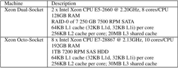
The sizes of the raw CSV and binary files are 28GB and 12GB respectively. The experiments are run on a dual socket Intel Xeon, described in the first row of Table 1. The operating system is Red Hat Enterprise Linux Server 6.3 with kernel version 2.6.32. The compiler used is GCC 4.4.7 (with flags -msse4 -O3 -ftree-vectorize -march=native -mtune=native). The files are memory-mapped. The first query runs over cold caches. Intermediate query results are cached and available for re-use by subsequent queries.

Machine Description

Xeon Dual-Socket 2 x Intel Xeon CPU E5-2660 @ 2.20GHz, 8 cores/CPU 128GB RAM

RAID-0 of 7 250 GB 7500 RPM SATA 64KB L1 cache (32KB L1d, 32KB L1i) per core 256KB L2 cache per core; 20MB L3 shared cache Xeon Octo-Socket 8 x Intel Xeon CPU E7-28867 @ 2.13GHz, 10 cores/CPU

192GB RAM

1TB 7200 RPM SAS HDD

64KB L1 cache (32KB L1d, 32KB L1i) per core 256KB L2 cache per core; 30MB L3 shared cache

Table 1: Hardware Setup for experiments

We run the microbenchmarks in RAW. The code generation is done by issuing C++ code through a layer of C++ macros.

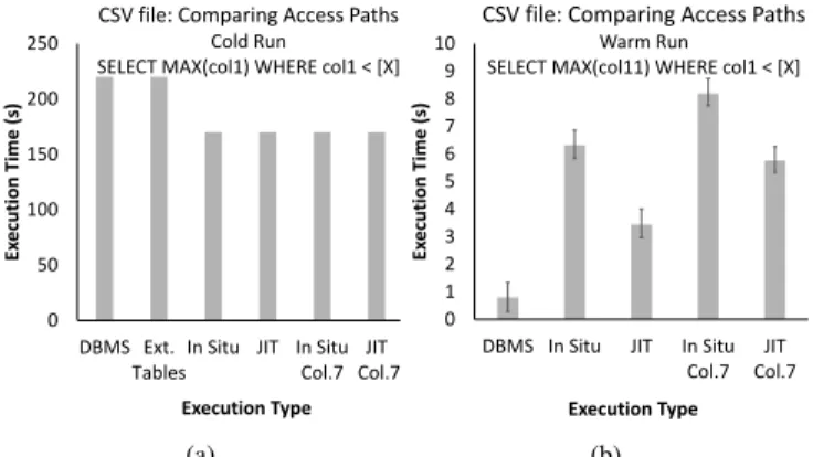
Data Loading vs. In Situ Query Processing. The follow-ing experiment compares different techniques, all implemented in RAW, for querying raw data to establish the trade-off between in situ query processing and traditional data loading. “DBMS” cor-responds to the behavior of a column-store DBMS, where all raw data is loaded before submitting the first query. The data loading time of the DBMS is included as part of the first query. “External Tables” queries the raw file from scratch for every query. “In Situ” is our implementation of NoDB [5] over RAW, where access paths arenotcode-generated. “JIT” corresponds to JIT access paths.

The workload comprises two queries submitted in sequence. The first isSELECT MAX(col1) WHERE col1 < [X], followed by SELECT MAX(col11) WHERE col1 < [X]. We report results for different selectivities by changing the value of X.

The first experiment queries a CSV file. “In Situ” and “JIT” both utilize positional maps, which are built during the execution of the first query and used in the second query to locate any missing columns. Because different policies for building positional maps are known to affect query performance [5], we test two different heuristics. The first populates the positional map every 10 columns; i.e., it tracks positions of columns 1, 11, 21, etc. The second popu-lates the positional map every 7 columns.

Figure 1a depicts the results for the first query (cold file sys-tem caches). The response time is approximately 220 seconds for “DBMS” and “External Tables” and 170 seconds for “In Situ” and “JIT”. “DBMS” and “External Tables” do the same amount of work for the first query, building an in-memory table with all data in the file before executing the query. “In Situ” and “JIT” do fewer data conversions and populate fewer columns (only those actually used by the query), which reduces the execution time. In the case of JIT access paths, the time to generate and compile the access path code

(6)

0 1 2 3 4 5 6 7 8 9 10

DBMS In Situ JIT In Situ Col.7 JIT Col.7 Ex ec ut ion Ti me (s) Execution Type

CSV file: Comparing Access Paths

Warm Run

SELECT MAX(col11) WHERE col1 < [X]

0 50 100 150 200 250 DBMS Ext. Tables

In Situ JIT In Situ Col.7 JIT Col.7 Ex ec ut ion Ti me (s) Execution Type

Cold Run

(a) 0 1 2 3 4 5 6 7 8 9 10

DBMS In Situ JIT In Situ Col.7 JIT Col.7 Ex ec ut ion Ti me (s) Execution Type

Warm Run

0 50 100 150 200 250 DBMS Ext. Tables

In Situ JIT In Situ Col.7 JIT Col.7 Ex ec ut ion Ti me (s) Execution Type

Cold Run

(b)

Figure 1: a) Raw data access is faster than loading (I/O masks part of the difference). b) “DBMS” is faster, as all needed data is already loaded. JIT access paths are faster than general-purpose in situ. is included in the execution time of the first query, contributing ap-proximately 2 seconds.In both cases, however, I/O dominates the response time and the benefit of JIT access paths is not particularly visible (except that the compilation time is amortized).

For the second query, the results are depicted in Figure 1b. We vary selectivity from 1% to 100% and depict the average response time, as well as deltas for lowest and highest response time. The ex-ecution time for “External Tables” is an order of magnitude slower, thus it is not shown. The “In Situ” and “JIT” cases use the po-sitional map to jump to the data in column 11. The variations “In Situ - Column 7” and “JIT - Column 7” need to parse incrementally from the nearest known position (column 7) to the desired column (column 11). In all cases, a custom version ofatoi(), the function used to convert strings to integers, is used as the length of the string is stored in the positional map. Despite these features, “DBMS” is faster, since data is already loaded into the columnar structures used by the query engine, whereas the “JIT” case spends approximately 80% of its execution on accessing raw data. It is important to note, however, that the extra loading time incurred by the “DBMS” dur-ing the first query may not be amortized by fast upcomdur-ing queries; these results corroborate the observations of the NoDB paper [5].

Comparing “In Situ” with “JIT”, we observe that the code gen-eration version is approximately 2×faster. This difference stems from the simpler code path in the generated code. The “In Situ -Column 7” and “JIT - -Column 7” techniques are slower as expected compared to their counterparts that query the mapped column 11 directly, due to the incremental parsing that needs to take place.

We now turn to the binary file. No positional map is necessary now. The “In Situ” version computes the positions of data elements during query execution. The “JIT” version hard-codes the positions of data elements into the generated code. For the first query, both “In Situ” and “JIT” take 70 seconds. The “DBMS” case takes 98 seconds. I/O again masks the differences between the three cases. The results for the second query are shown in Figure 2. The trends of all cases are similar to the CSV experiment. The performance gaps are smaller because no data conversions take place.

JIT access paths breakdown. To confirm the root cause of speedup in the “JIT” case, we profile the system using VTune2_.

We use the same CSV dataset as before, and ask the querySELECT MAX(col1) WHERE col1 <[X]on a warm system. Figure 3 shows the comparison of the “JIT” and “In Situ” cases for a case with 40% selectivity. Unrolling the main loop, simplifying the parsing code and the data type conversion reduces the costs of accessing raw data. Populating columns and parsing the file remain expensive

2_{http://software.intel.com/en-us/intel-vtune-amplifier-xe} 0 0.5 1 1.5 2 2.5 3 3.5 4 0% 10% 20% 30% 40% 50% 60% 70% 80% 90% 100% Ex ecution Time (s) Selectivity

Binary file: Comparing Access Paths SELECT MAX(col11) WHERE col1 < [X]

In Situ JIT DBMS

Figure 2: For binary files, JIT access paths are also faster for the 2nd query than traditional in situ query processing.

0g 10g 20g 30g 40g 50g 60g 70g 80g 90g 100g In Situ JIT Tot al C os t BreakdowncofcQuerycExecutioncCosts MaincLoop Parsing DatacType BuildcColumns

Figure 3: Unrolling the main loop, simplifying parsing and data type conversions reduce the time spent “preparing” raw data.

though. In the next section we introduce column shreds to reduce these costs.

Discussion. JIT access paths significantly reduce the overhead of in situ query processing. For CSV files and for a custom-made binary format, JIT access paths are up to 2×faster than traditional in situ query processing techniques. Traditional in situ query pro-cessing, adapted to columnar execution, is affected by the general-purpose and query-agnostic nature of the scan operators that ac-cess raw data. Just-In-Time code generation, however, introduces a compilation overhead, incurred the first time a specific query is asked. Two methods to address this issue are i) maintaining a “cache” of libraries generated as a side-effect of previous queries, and re-using when applicable (RAW follows such an approach), and ii) using a JIT compiler framework, such as LLVM [24], which can reduce compilation times [30].

As we see in the next section, the flexibility and efficiency of-fered by JIT access paths combined with column shreds will enable us to further increase the performance of RAW.

5. WHEN TO LOAD DATA

JIT access paths reduce the cost of accessing raw data. There are, however, inherent costs with raw data access that cannot be removed despite the use of JIT access paths. These costs include i) multiple accesses to the raw files, ii) converting data from the file format (e.g., text) to the database format (e.g., C types), and iii) creating data structures to place the converted data.

Use of column shreds is a novel approach that further reduces the cost of accessing raw data. So far, we have been considering the traditional scenario in which we have a scan operator per file, reading the fields required to answer a query and building columns of values. Column shreds build upon the flexibility offered by JIT scan operators. Specifically, we can generate multiple operators for

(7)

Scan CSV Columns 1,2 Filter Tuple Construction Col1 Col2 Col1

FULL COLUMNS COLUMN SHREDS

Scan CSV Column 1 Filter Scan CSV Column 2 Tuple Construction Col1 Col2 Col1 Col2 Col1 [1,3,4] Col1 Col2

Figure 4: “Full columns”: all columns are pre-loaded into the database system’s columnar structure. “Column shreds”: column pieces are only built as needed: in the example, Col2 is only loaded with the rows that passed the filter condition on Col1.

a single data source, each reading an arbitrary subset of fields in a row-wise manner from the file. Our aim is to have each operator read the minimum amount of data required at the time. To achieve this, based on when a field is used by a query operator (e.g., it is used in a join predicate), we place the scan operator reading the field valueshigher in the query plan, in hope that many results will have been filtered out by the time the operator is launched. As a result, instead of creating columns containing all the values of a raw file’s requested fields, we end up creatingshreds of the columns.

In the rest of this section, we present column shreds and eval-uate their behavior. We consider the applicability of using col-umn shreds in different scenarios, gauge their effects and isolate the criteria indicating when they should be applied.

5.1 Shredding Columns

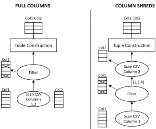
Creating entire columns at startup is a conceptually simple ap-proach. A small experiment, however, illustrates the potential over-head it carries. Assume a query such asSELECT MAX(col2) FROM table WHERE col1 < N. The number of entries from col2 that need to be processed to compute theMAXdepend on the selectiv-ity of the predicate on col1. If columns 1 and 2 are entirely loaded, in what we now call“full columns”, then some elements of column 2 will be loaded but never used. If the selectivity of the predicate is 5%, then 95% of the entries read from column 2 will be unnec-essary for the query. This is an undesirable situation, as time is spent on creating data structures and loading them with data that is potentially never needed but still expensive to load.

The “column shreds” approach dictates creating and populating columns with data only when that data is strictly needed. In the previous example, we load only the entries of column 2 that qualify, i.e., if the selectivity of the predicate is 5%, then only 5% of the entries for column 2 are loaded, greatly reducing raw data accesses. Figure 4 illustrates the difference between the two column cre-ation strategies. In the case of full columns, a single scan operator populates all required columns. For this example, column shreds are implemented by generating a columnar scan operator for col-umn 2 and pushing itup the query plan. In addition, the (Just-In-Time) scan operators are modified to take as input the identifiers of qualifying rows from which values should be read. In Figure 4 this is the set of rows that pass the filter condition. For CSV files, this

selection vector[9] actually contains the closest known binary po-sition for each value needed, as obtained from the popo-sitional map. The remaining query plan and operators are not modified.

It is important for the multiple scan operators accessing a file to work in unison. For the majority of file formats, reading a field’s values from a file requires reading a file page containing unneeded data. Therefore, when a page of the raw file is brought in memory due to an operator’s request, we want to extract all necessary infor-mation from it and avoid having to re-fetch it later. Our operators accept and produce vectors of values as input and output respec-tively. After a scan operator has fetched a page and filled a vector with some of the page’s contents, it forwards the vector higher in the query tree. Generally, at the time a subsequent scan operator requests the same file page to fill additional vectors, the page is still “hot” in memory, so we do not incur I/O again. If we had opted for operators accepting full columns, we would not avoid duplicate I/O requests for pages of very large files.

RAW maintains a pool of previously created column shreds. A shred is used by an upcoming query if the values it contains sub-sume the values requested. The replacement policy we use for this cache is LRU. Handling the increasing number of varying-length shreds after a large number of queries and fully integrating their use can introduce bookkeeping overheads. Efficient techniques to handle this can be derived by considering query recycling of inter-mediate results, as applied in column stores [18, 29].

5.2 Full Columns vs. Column Shreds

To evaluate the behavior of column shreds, we compare them with the traditional “full columns” approach. The hardware and workload used are the same as in Section 4. We use simple an-alytical queries of varying selectivity so that the effect of full vs shredded columns is easily quantifiable, instead of being mixed with other effects in the query execution time. All cases use JIT access paths. For CSV files, a positional map is built while running the first query and used for the second query. As in Section 4 we include two variations of the positional map: one where the posi-tional map tracks the position of a column requested by the second query, and one where the positional map tracks a nearby position.

The execution time of the first query is not shown because there is no difference between full and shredded columns: in both cases, every element of column 1 has to be read. Figure 5 shows the ex-ecution time for the second query over the CSV file of 30 columns and 100 million rows. For lower selectivities, column shreds are significantly faster (∼6×) than full columns, because only the el-ements of column 11 that pass the predicate on column 1 are read from the raw file. Compared to the traditional in situ approach evaluated in Section 4, the improvement reaches∼12×. As the selectivity increases, the behavior of column shreds converges to that of full columns. Column shreds are always better than full columns, or exactly the same for 100% selectivity. When incre-mental parsing is needed, then data is uniformly more expensive to access. In all cases, the extra work in the aggregator operator, which has more data to aggregate as the selectivity increases, con-tributes to the gradual increase in execution time. Compared to the DBMS case, however, the increase for full and shredded columns is steeper. The reason is that reading the file and aggregating data are done at the same time and both actions interfere with each other.

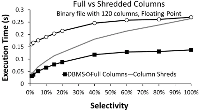
For binary files, the same behavior is observed (Figure 6). Al-though no data conversion takes place, the other loading-related costs, e.g., populating columns, still affect the “full columns” case. The next set of experiments uses files with wider tables (more columns) and more data types, including floating-point numbers. There are now 120 columns in each file and 30 million rows. The sizes of the CSV and binary files are 45GB and 14GB respectively. In the traditional DBMS case, all columns in the file are created before launching queries. In the “full columns” case, all columns

(8)

0 1 2 3 4 5 6 7 0% 10% 20% 30% 40% 50% 60% 70% 80% 90% 100% Ex ecution Time (s) Selectivity

Full vs Shredded Columns CSV file; SELECT MAX(col11) WHERE col1 < [X]

Full Shreds Full - Column 7 Shreds - Column 7 DBMS Figure 5: For the 2nd query over a CSV file, column shreds are always faster or exactly the same as full columns, as only elements of column 11 that pass the predicate are loaded from the file.

0 0.5 1 1.5 2 2.5 3 3.5 4 0% 10% 20% 30% 40% 50% 60% 70% 80% 90% 100% Ex ecution Time (s) Selectivity

Full vs Shredded Columns Binary file; SELECT MAX(col11) WHERE col1 < [X]

Full Shreds

Figure 6: For the 2nd query over a binary file, we see the same behavior as for CSV: use of column shreds is always faster than use of full columns or exactly the same for 100% selectivity.

0 2 4 6 8 10 0% 10% 20% 30% 40% 50% 60% 70% 80% 90% 100% Ex ecution Time (s) Selectivity

Full vs Shredded Columns CSV file with 120 columns, Floating-Point DBMS Full Columns Column Shreds

Figure 7: CSV files with floating-point numbers carry a higher data type conversion cost. The DBMS case is significantly faster.

0 0.05 0.1 0.15 0.2 0.25 0.3 0% 10% 20% 30% 40% 50% 60% 70% 80% 90% 100% Ex ecution Time (s) Selectivity

Full vs Shredded Columns Binary file with 120 columns, Floating-Point

DBMS Full Columns Column Shreds

Figure 8: The binary format requires no conversions, so the abso-lute difference between DBMS and column shreds is very small.

needed by the query are created as the first step of a query. In the “column shreds” case, columns are only created when needed by some operator. In the “DBMS” case, the loading time is included in the execution time of the first query. Column 1, with the predicate condition, is an integer as before. The column being aggregated is now a floating-point number, which carries a greater data type conversion cost. The queries and remaining experimental setup are the same as before.

System File Format Execution Time (s)

DBMS CSV 380 s

Full Columns CSV 216 s

Column Shreds CSV 216 s

DBMS Binary 42 s

Full Columns Binary 22 s

Column Shreds Binary 22 s

Table 2: Execution time of the 1st query over a table with 120 columns of integers and floating-point numbers. A traditional DBMS is significantly slower in the 1st query due to data loading.

Table 2 shows the execution times for the first query. For CSV files, although I/O masks a significant part of the cost, the DBMS is 164 seconds slower, as it loads (and converts) all columns in ad-vance, even those not part of subsequent queries. Full and shredded columns are the same for the first query, as the entire column must be read to answer it. For binary files, the first query is nearly 2×

slower for the DBMS. Interestingly, we may also compare the CSV and binary file formats directly. Both hold the same data, just in dif-ferent representations. Querying CSV is significantly slower due to

the higher cost of converting raw data into floating-point numbers and the larger file size.

The execution times for the second query in the case of the CSV file are shown in Figure 7. Using column shreds is competitive with “DBMS” only for lower selectivities. The curve gets steeper due to the higher cost of converting raw data into floating-point numbers. In the binary case (Figure 8) there is no need for data type con-versions. Therefore, use of column shreds is competitive with the DBMS case for a wider range of selectivities. It is approximately 2×slower for 100% selectivities, yet the absolute time differences are small. The slowdown is due to building the in-memory colum-nar structures, and could only be resolved if the entire set of database operators could operate directly over raw data.

5.3 Column Shreds Tradeoffs

So far we examined simple analytical queries with the goal of isolating the effects of shredding columns of raw data. Intuitively, postponing work as long as possible in the hope that it can be avoided appears to be always of benefit. In this section, we ex-amine whether this assumption is true for other types of queries.

5.3.1 Speculative Column Shreds

For some file formats, the strict form of using scan operators to create column shreds for a single field each time may not be desirable. For example, when reading a field from a file, it may be comparatively cheap to read nearby fields. If these nearby fields are also needed by the query - e.g., they are part of a predicate selection to be executed upstream - then it may be preferable tospeculatively

read them to reduce access costs (e.g., parsing).

In the next experiment we ask the querySELECT MAX(col6) FROM file1 WHERE file1.col1 <[X] AND file1.col5 <[X]

(9)

0 2 4 6 8 10 12 0% 10% 20% 30% 40% 50% 60% 70% 80% 90% 100% Ex ecution Time (s) Selectivity

Full vs Shreds vs Multi-column Shreds SELECT MAX(col6) WHERE col1 < [X] AND col5 < [X]

Full Shreds Multi-column Shreds

Figure 9: Creating shreds of requested nearby columns in one step is beneficial when accessing raw data in multiple steps is costly.

over a CSV file. A positional map already exists (for columns 1 and 10), and the data for column 1 has been cached by a previous query. We compare three cases:

• full columns for fields 5 and 6 (column 1 is already cached)

• a column shred for field 5 (after predicate on field 1) and a col-umn shred for field 6 (after predicate on field 5)

• column shreds for fields 5 and 6 after predicate on column 1 (i.e.,

“multi-column shreds”) using a single operator

As depicted in Figure 9, for selectivities up to 40%, creating one column shred each time is faster because we process less data. Af-ter this point, the parsing costs begin to dominate and override any benefit. The intermediate case, however, provides the best of both cases: if we speculatively create the column shred for field 6 at the same time as the one for field 5, the tokenizing/parsing cost is very small. Pushing the scan operator for field 6 higher means that the system loses “locality” while reading raw data.

5.3.2 Column Shreds and Joins

For queries with joins, column shreds can also be beneficial. For some file formats, however, we must carefully consider where to place the scan operator. Intuitively, columns to be projected after the join operator should be created on demand as well. That is, the join condition would filter some elements and the new columns to be projected would only be populated with those elements of inter-est that passed the join condition. In practice, there is an additional effect to consider, and in certain scenarios it is advantageous to cre-ate such a column before the join operator.

When considering hash joins, the right-hand side of the join is used to build a hashtable. The left-hand side probes this hashtable in a pipelined fashion. The materialized result of the join includes the qualifying probe-side tuples in their original order, along with the matches in the hashtable.

Let us consider the querySELECT MAX(col11) FROM file1, file2 WHERE file1.col1=file2.col1 AND file2.col2<[X] over two CSV files. Both file1 and file2 contain the same data, but file2 has been shuffled. We examine the cases in which an addi-tional column to be projected belongs to file1 (left-hand side of the join) or to file2 (right-hand side of the join). We assume that col-umn 1 of file1 and colcol-umns 1 and 2 of file2 have been loaded by previous queries, to isolate the direct cost of each case. We change X to alter the number of rows from file2 participating in the join.

Both cases are shown in Figure 10. The “Pipelined” case corre-sponds to retrieving the projected column from file1 and the “Pipe-line Breaking” to retrieving it from file2. Both cases have two

Scan File1 Column 1 Scan File2 Columns 1,2 File1.Col1 ⨝File2.Col1 Col2 Col1 File1.Col11 PIPELINED PIPELINE-BREAKING Filter Column 2 Col1 File2 File1 Col1 Col2 Scan File1 Column 11 Late Scan File1 Column 1 Scan File2 Columns 1,2 File1.Col1 ⨝File2.Col1 Col2 Col1 File2.Col11 Filter Column 2 Col1 File2 File1 Col1 Col2 Scan File2 Column 11 Late

Figure 10: Possible points of column creation based on join side.

0 5 10 15 20 25 30 35 40 1% 10% 20% 40% 60% 80% 100% Ex ec utio n Time (s) Selectivity

Join w/ projected column on the left-hand side (pipelined)

Early Late DBMS 0 5 10 15 20 25 30 35 40 45 50 55 1% 10% 20% 40% 60% 80% 100% Ex ec utio n Time (s) Selectivity

Join w/ projected column on the right-hand side (pipeline-breaking)

Early Late Intermediate DBMS

Figure 11: If the column to be projected is on the “pipelined” side of the join, then delaying its creation is a better option.

0 5 10 15 20 25 30 35 40 1% 10% 20% 40% 60% 80% 100% Ex ec utio n Time (s) Selectivity

Join w/ projected column on the left-hand side (pipelined)

Early Late DBMS 0 5 10 15 20 25 30 35 40 45 50 55 1% 10% 20% 40% 60% 80% 100% Ex ec utio n Time (s) Selectivity

Join w/ projected column on the right-hand side (pipeline-breaking)

Early Late Intermediate DBMS

Figure 12: If the projected col-umn is on the “breaking” side, picking its point of creation de-pends on the join selectivity.

common points in the query plan where the column to be pro-jected can be created; these are called “Early” and “Late” in Fig-ure 10. The “Early” case is before the join operator (i.e., full columns); the “Late” case is after (i.e., column shreds). In the “Pipeline-Breaking” scenario, we also identify the “Intermediate” case, where we push the scan of the projected column after having applied all selection predicates, yet before applying the join. The result is creating shreds which may carry some redundant values.

The first experiment examines the “Pipelined” case. Two copies of the original CSV dataset with 100 million rows are used. The second copy is shuffled. The results are shown in Figure 11, also in-cluding the default “DBMS” execution for reference. The behavior is similar to that of full vs. shredded columns for selection queries: column shreds outperform full columns when selectivity is low, and the two approaches converge as selectivity increases. The reason is that the ordering of the output tuples of the join operator follows the order of entries in file1. The pipeline is not broken: therefore, the scan operator for column 11, which is executed (pipelined) af-ter the join operator, reads the qualifying entries via the positional map in sequential order from file1. We also notice that for complex operations such as joins, the fact that we access raw data is almost entirely masked due to the cost of the operation itself and the use of column shreds. For small selectivities we observe little difference.

The second experiment examines the remaining case, which we call “Pipeline-breaking”. The column to be projected is now from file2. The results are shown in Figure 12. DBMS, full and shred-ded columns perform worse than their pipelining counterparts. As the selectivity of the query increases, the performance of column shreds deteriorates, eventually becoming worse than full columns.

(10)

The intermediate case exhibits similar behavior, but is not as heav-ily penalized for high selectivities as the late case. The reason for this behavior are non-sequential memory accesses when reading the data. In the “DBMS” and “full columns” cases, column values are not retrieved in order, as they have been shuffled by the join operation. Even worse, in the case of column shreds it is the byte positions of the raw values stored in the positional map that have been shuffled. This leads to random accesses to the file (or to the memory-mapped region of the file). Pages loaded from the file, that already contain lots of data not needed for the query (as opposed to tight columns in the case of “full columns”), may have to be read multiple times during the query to retrieve all relevant values. This sub-optimal access pattern ends up overriding any benefits obtained from accessing a subset of column 11 in the case of column shreds. To confirm this behavior, we use theperf3performance analyz-ing tool to measure the number of DTLB misses in the “pipeline-breaking” scenario. We examine the two “extreme” cases for an in-stance of the query with 60% selectivity. Indeed, the “full columns” case has 900 million DTLB misses and 1 billion LLC misses, while the “column shreds” case has 1.1 billion DTLB misses and 1.1 bil-lion LLC misses due to the random accesses to the raw data.

Discussion. The use of column shreds is an intuitive strategy that can provide performance gains for both selection queries and joins, where the gains are a function of query selectivity. Column shreds, however, cannot be applied naively, as loading data without con-sidering locality effects can increase the per-attribute reading cost. In such cases of higher selectivity, multi-column shreds for selec-tions, and full creation of newly projected columns that break the join pipeline for joins, provide the best behavior in our experiments.

6. USE CASE: THE HIGGS BOSON

The benchmarks presented in the previous sections demonstrate that JIT access paths combined with column shreds can reduce the costs of querying raw data. In practice, however, the impact of these methods depends on the specificities of each file format. Be-cause we cannot possibly evaluate our techniques with the multi-tude of file formats and workloads in widespread use, we instead identify one challenging real-world scenario where data is stored in raw files and where DBMS-like query capabilities are desirable.

The ATLAS experiment [1] at CERN manages over 140 PB of data. ATLAS is not using a DBMS because of two non-functional requirements, namely i) the lifetime of the experiment: data should remain accessible for many decades; therefore, vendor lock-in is a problem, and ii) the dataset size and its associated cost: storing over 140 PB in a DBMS is a non-trivial, expensive task.

The ATLAS experiment built a custom data analysis infrastruc-ture instead of using a traditional DBMS. At its core is the ROOT framework[10], widely used in high-energy physics, which includes its own file format and provides a rich data model with support for table-like structures, arrays or trees. ROOT stores data in a variety of layouts, including a columnar layout with optional use of com-pression. The framework also includes libraries to serialize C++ objects to disk, handles I/O operations transparently and imple-ments an in-memory “buffer pool” of commonly-accessed objects. To analyze data, ATLAS physicists write custom C++ programs, extensively using ROOT libraries. Each such program “implements” a query, which typically consists of reading C++ objects stored in a ROOT file, filtering its attributes, reading and filtering nested ob-jects, projecting attributes of interest and usually aggregating the final results into a histogram. ROOT does not provide declarative

3_{https://perf.wiki.kernel.org} Jet eventID INT eta FLOAT pt FLOAT Event eventID INT runNumber INT Electron eventID INT eta FLOAT pt FLOAT Muon eventID INT eta FLOAT pt FLOAT class Event { class Muon { float pt; float eta; … } class Electron { float pt; float eta; … } class Jet { float pt; float eta; … } int runNumber; vector<Muon> muons; vector<Electron> electrons; vector<Jet> jets; } ROOT - C++ RAW

Figure 13: Data representation in ROOT and RAW. RAW represen-tation allows vectorized processing.

querying capabilities; instead, users code directly in C++, using ROOT to manage a buffer pool of C++ objects transparently.

In an ideal scenario, physicists would write queries in a declara-tive query language such as SQL. Queries are easier to express in a declarative query language for the average user. Query optimiza-tion also becomes possible, with the query engine determining the most appropriate way to execute the query.

To test the real-world applicability of querying raw data based on JIT access paths and column shreds, we implement a query of the ATLAS experiment (“Find the Higgs Boson”) in RAW. The JIT ac-cess paths in RAW emit code that calls the ROOT I/O API, instead of emitting code that directly interprets the bytes of the ROOT for-mat on disk. The emitted code calls ROOT’sgetEntry()method to read a field instead of parsing the raw bytes, as the ROOT for-mat is complex and creating a general-purpose code generator for ROOT would have been time-consuming. At the same time, code generation does allow us to plug existing libraries easily.

Because ROOT is a binary format where the location of every attribute is known or can be computed in advance, a positional map is not required. Instead, the code generation step queries the ROOT library for internal ROOT-specific identifiers that uniquely identify each attribute. These identifiers are placed into the generated code. In practice, the JIT access path knows the location and can access each data element directly. We utilize the ROOT I/O API to gen-erate scan operators that are performing identifier-based accesses (e.g., leading to a call of readROOTField(name,10) for a field’s en-try with ID equal to 10), thus pushing some filtering downwards, avoiding full scans and touching less data.

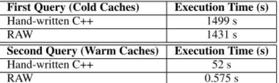
For this experiment, each ATLAS ROOT file contains informa-tion for a set of events, where an event is an observainforma-tion of a col-lision of two highly energized particles. The Higgs query filters events where the muons, jets and electrons in each event pass a set of conditions, and where each event contains a given number of muons/jets/electrons. In the hand-written version, an event, muon, jet or electron is represented as a C++ class. A ROOT file contains a list of events, i.e., a list of C++ objects of type event, each contain-ing within a list of C++ objects for its correspondcontain-ing muons, jets, electrons. In RAW, these are modelled as the tables depicted in Fig-ure 13. Therefore, the query in RAW filters the event table, each of the muons/jets/electrons satellite tables, joins them, performs ag-gregations in each and filters the results of the agag-gregations. The events that pass all conditions are the Higgs candidates.

The dataset used is stored in 127 ROOT files, totaling 900 GB of data. Additionally, there is a CSV file representing a table, which contains the numbers of the “good runs”, i.e., the events detected by the ATLAS detector that were later determined to be valid.