Exploring Compositional Data with the
CoDa-Dendrogram
Vera Pawlowsky-Glahn
1and Juan Jose Egozcue
21
University of Girona, Spain
2
Technical University of Catalonia, Barcelona, Spain
Abstract: Within the special geometry of the simplex, the sample space of compositional data, compositionalorthonormal coordinates allow the appli-cation of any multivariate statistical approach. The search for meaningful coordinates has suggested balances (between two groups of parts)—based on a sequential binary partition of aD-part composition—and a representa-tion in form of a CoDa-dendrogram. Projected samples are represented in a dendrogram-like graph showing: (a) the way of grouping parts; (b) the ex-planatory role of subcompositions generated in the partition process; (c) the decomposition of the variance; (d) the center and quantiles of each balance. The representation is useful for the interpretation of balances and to describe the sample in a single diagram independently of the number of parts. Also, samples of two or more populations, as well as several samples from the same population, can be represented in the same graph, as long as they have the same parts registered. The approach is illustrated with an example of food consumption in Europe.
Keywords: Aitchison Geometry, Euclidean Vector Space, Orthonormal Co-ordinates.
1
Introduction
The sample space of D-part compositional data, the simplex, being a subset of the real space RD, has a real Euclidean vector space structure (Billheimer, Guttorp, and Fagan,
2001; Pawlowsky-Glahn and Egozcue, 2001). The easiest way to study data whose sam-ple space is a real Euclidean space is to represent them in coordinates with respect to an orthonormal basis. Coordinates behave like real random vectors (Kolmogorov and Fomin, 1957) and thus, as discussed in Pawlowsky-Glahn (2003), any usual statistical technique can be applied. In any Euclidean space, an infinite number of orthonormal bases exists, and the simplex is one of them. Different techniques can be used to build such a basis. The best known techniques in mathematics use the Gram-Schmidt orthonormalisation process or a Singular Value Decomposition (Egozcue, Pawlowsky-Glahn, Mateu-Figueras, and Barcel´o-Vidal, 2003). These mathematically straightforward methods, however, not al-ways lead to easy-to-interpret coordinates.
The analysis of problems related to the amalgamation of parts, and the search for di-mension reducing techniques related to subcompositions, suggested a new strategy: bal-ances. Balances are a specific kind of orthonormal coordinates associated with groups of parts (Egozcue and Pawlowsky-Glahn, 2005b). They are based on a sequential binary partition of a D-part composition into non-overlapping groups. This approach is very
intuitive and the resulting coordinates are frequently easy to interpret. Moreover, it leads to a decomposition of the total variance into marginal variances which can be assigned either to intra-group (subcompositional) variability, or to inter-group variability (relative variability between two groups of parts). To visualise this, together with other univariate characteristics, a specific tool, the CoDa-dendrogram, has been developed.
2
A Compositional Data Set
To present the approach from an intuitive perspective, let us consider the following prob-lem: To decide his business strategy, one merchant, leader in the food industry, wants to compare the food consumption habits in the old East and the West countries. To do so, he wants to analyse data—published by Eurostat (Pe˜na, 2002)—reproduced in Table 1. These data are percentages of consumption of 9 different kinds of food in 25 countries in Europe in the early eighties. A preliminary question is which is the relevant information Table 1: Food consumption expenditure in the East (E) and the West (W), published by Eurostat, in percent. The sample size is 25. Legend:RM: red meat;WM: white meat;F: fish;E: eggs;M: milk;C: cereals;S: starch;N: nuts;FV: fruit and vegetables.
RM WM E M F C S N FV group country 10.1 1.4 0.5 8.9 0.2 42.3 0.6 5.5 1.7 E Albania 8.9 14.0 4.3 19.9 2.1 28.0 3.6 1.3 4.3 W Austria 13.5 9.3 4.1 17.5 4.5 26.6 5.7 2.1 4.0 W Belgium 7.8 6.0 1.6 8.3 1.2 56.7 1.1 3.7 4.2 E Bulgaria 9.7 11.4 2.8 12.5 2.0 34.3 5.0 1.1 4.0 E Check Rep. 10.6 10.8 3.7 25.0 9.9 21.9 4.8 0.7 2.4 W Denmark 9.5 4.9 2.7 33.7 5.8 26.3 5.1 1.0 1.4 W Finland 18.0 9.9 3.3 19.5 5.7 28.1 4.8 2.4 6.5 W France 9.3 4.6 2.1 16.6 3.0 43.6 6.4 3.4 2.9 E FSU 8.4 11.6 3.7 11.1 5.4 24.6 6.5 0.8 3.6 E Germany (E) 11.4 12.5 4.1 18.8 3.4 18.6 5.2 1.5 3.8 W Germany (W) 10.2 3.0 2.8 17.6 5.9 41.7 2.2 7.8 6.5 W Greece 5.3 12.4 2.9 9.7 0.3 40.1 4.0 5.4 4.2 E Hungary 13.9 10.0 4.7 25.8 2.2 24.0 6.2 1.6 2.9 W Ireland 9.0 5.1 2.9 13.7 3.4 36.8 2.1 4.3 6.7 W Italy 9.4 4.7 2.7 23.3 9.7 23.0 4.6 1.6 2.7 W Norway 6.9 10.2 2.7 19.3 3.0 36.1 5.9 2.0 6.6 E Poland 6.2 3.7 1.1 4.9 14.2 27.0 5.9 4.7 7.9 W Portugal 6.2 6.3 1.5 11.1 1.0 49.6 3.1 5.3 2.8 E Rumania 7.1 3.4 3.1 8.6 7.0 29.2 5.7 5.9 7.2 W Spain 9.9 7.8 3.5 24.7 7.5 19.5 3.7 1.4 2.0 W Sweden 13.1 10.1 3.1 23.8 2.3 25.6 2.8 2.4 4.9 W Switzerland 9.5 13.6 3.6 23.4 2.5 22.4 4.2 1.8 3.7 W The Netherlands 17.4 5.7 4.7 20.6 4.3 24.3 4.7 3.4 3.3 W United Kingdom 4.4 5.0 1.2 9.5 0.6 55.9 3.0 5.7 3.2 E Yugoslavia
in this data set and which is the sample space of the data. Although data are presented here as percentages of expenditure, it is not clear what is the meaning of total expenditure or how it was measured. Moreover, each data-vector does not add to 100%. This means that there is an implicitly defined additional component, that we callother, that completes the total, i.e. 100%. Even more, we have doubts about the units of expenditure: if they are measured in different currencies, how have the reference prices been established? Also, if the units were tons of food of each type, what would the meaning of the above percent-ages be? What does a percentage of tons of a total, made of tons of meat plus tons of nuts, mean? These questions lead to two important conclusions:
• The definition of the total is irrelevant, both with respect to its units and to the reported components constituting the data-vector.
• The information to be extracted from such a data-set is not related to the units in which the original components were registered.
These points match the so called principles of compositional data analysis (Aitchison, 1986; Aitchison and Egozcue, 2005; Egozcue, 2009). They can be summarized asscale invariance and subcompositional coherence. The first one states that a change of units should not alter compositional information. The second one advocates that a change of scale should be applicable to any subset of two or more components, called subcomposi-tion; also, that conclusions obtained from a subcomposition should not be in contradiction with those obtained from a composition including it. For instance, if an analyst studies the parts of animal based food (meat, fish, . . . ), he should not reach a conclusion which stands in contradiction with the conclusions of another analyst dealing with the whole composition. The key point of these principles is that the only information conveyed by compositional data are the ratios between the different parts of the observed composition. This is the case of the data-set presented in Table 1 and they should be considered as a compositional data-set. Therefore, the sample space of the food consumption is the 9 -part simplex, S9. In order to represent the data set in the simplex, the closure operation is used: if x = (x1, x2, . . . , x9) is one of the data vectors and t =
∑9
j=1xj, then the
closed vector isCx= (x1/t, x2/t, . . . , x9/t), so that its components, called parts, add to 1. In this case, they are expressed in parts per unit. To obtain a different closure con-stant, the resulting closed vector has to be multiplied by the corresponding constant; e.g.
κ = 100 gives percentages. The vectorsxandCxare said to be compositionally equiv-alent (Barcel´o-Vidal, Mart´ın-Fern´andez, and Pawlowsky-Glahn, 2001). The importance of the closure is only apparent. The whole compositional analysis is based on the scale invariance and all characteristics of a composition are invariant under a multiplication by a positive constant.
Another important point in compositional analysis is that the distances in the simplex, called Aitchison distances, are invariant under perturbation. Perturbation of a composition ofDparts,x, by aD-vector with positive components,p, is defined as the composition
x⊕p=C(x1p1, x2p2, . . . , xDpD)
inSD. Perturbation is the addition in the Aitchison geometry of the simplex and can be viewed as a shift ofxbyp.
The Aitchison geometry of the simplex provides a distance between two compositions, da(x,y) = 1 D ∑ i<j ( log xi xj −log yi yj )2 ,
which is invariant under perturbations, i.e.
da(x,y) = da(x⊕p,y⊕p). (1)
This means that expressing the food expenditure in percent of some currency can be trans-formed by a perturbation into percent of tonnage of food. The components of the pertur-bation are simply the number of tons of each kind of food per unit of currency. Equation (1) implies that a change of units in the food consumption is a shift in the Aitchison geometry that preserves the inter-distances between compositions.
Once the sample space is identified as the simplexS9with its Aitchison geometry, the first statistical elements, namely the mean and variance-covariance, can also be identified (Aitchison, 1997; Pawlowsky-Glahn and Egozcue, 2001, 2002). For instance, the center of a random compositionxis defined as
Cen(x) =Cexp(E(logx)),
where the functionsexpandlogare applied to vectors componentwise. An important fact in the present example is that the center is shift compatible, as any well defined mean, i.e.
Cen(x⊕p) = Cen(x)⊕p.
Thus, a change of units from food expenditure in currency to tonnage causes the same change in the center.
The total variance of a random compositionx∈ SD is defined as
totVar(x) = E[d2a(x,Cen(x))]. (2)
It generalises the definition of variance in real space in the univariate case, when the Aitchison distance is replaced by the ordinary Euclidean distance. The total variance is easily expressed using orthogonal coordinates with respect to an orthonormal basis of the simplex. The function assigning to a compositionxa(D−1)-vector of real coordinates with respect to an orthonormal basis,c = (c1, c2, . . . , cD−1), is called isometric log-ratio transformation (ilr) (Egozcue et al., 2003). As the name isometric suggests, operations and distances in the simplex are transformed to their counterparts in the real space of coordinates, e.g. forx,yinSD
ilr(x⊕y) = ilr(x) + ilr(y), da(x,y) = d(ilr(x),ilr(y)),
whereddenotes the ordinary Euclidean distance inRD−1. Ifc = (c1, c2, . . . , cD−1)are the random coordinates of the random compositionx, i.e.c= ilr(x), the total variance of xis
totVar(x) =
D∑−1 j=1
where Var(ci) is the ordinary variance of the real random variable ci. The total
vari-ance has two important properties: it is invariant under perturbation, totVar(x⊕p) = totVar(x); and is also invariant under a change of basis. The variability ofxis fully de-scribed by the variance-covariance matrix of its coordinatesc. Again, the units in which the parts of food consumption were expressed are irrelevant for the analysis of the vari-ability.
3
Sequential Binary Partition
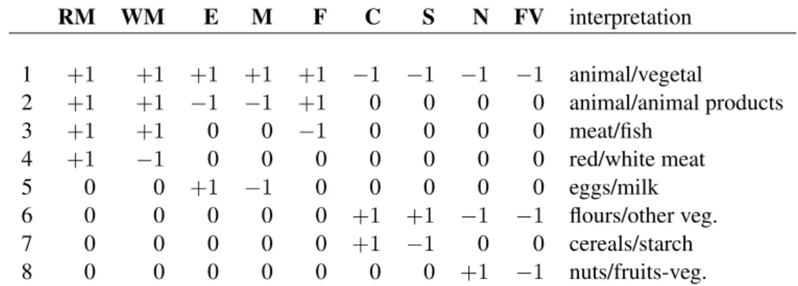
A useful way to build up an orthonormal basis of the simplex whose coordinates may be easily interpretable is to define a sequential binary partition (SBP) of the compositional vector. An SBP consists in a grouping of parts (Egozcue and Pawlowsky-Glahn, 2005b). A possible, user-defined, SBP is represented in Table 2. Each row corresponds to an order
Table 2: Sequential binary partition code: see text for details.
RM WM E M F C S N FV interpretation 1 +1 +1 +1 +1 +1 −1 −1 −1 −1 animal/vegetal 2 +1 +1 −1 −1 +1 0 0 0 0 animal/animal products 3 +1 +1 0 0 −1 0 0 0 0 meat/fish 4 +1 −1 0 0 0 0 0 0 0 red/white meat 5 0 0 +1 −1 0 0 0 0 0 eggs/milk 6 0 0 0 0 0 +1 +1 −1 −1 flours/other veg. 7 0 0 0 0 0 +1 −1 0 0 cereals/starch 8 0 0 0 0 0 0 0 +1 −1 nuts/fruits-veg.
iof partition,+1stands for inclusion in group of partsGi1, −1for inclusion in group of parts Gi2, and 0for no inclusion. At each step, a group of parts is partitioned into two non-overlapping groups. For example, the first step divides the food consumption into animal vs. vegetal origin,
G11={RM,WM,E,M,F} G12={C,S,N,FV},
while the second step divides the food of animal origin into animal and animal products
G21 ={RM,WM,F}, G22 ={E,M},
withG21∪G22=G11andG21∩G22 =∅. Note that, once a part appears as a single-part group, it does not appear again and the code is0at subsequent orders of partition.
4
Balances
Balances are the coordinates which represent an element of the simplex in the orthonormal basis defined by an SBP (Egozcue and Pawlowsky-Glahn, 2005b). In practice, there is
no need to know the exact expression of this basis, as the coordinates are computed using a one-to-one transformation (the correspondingilr) and for values of interest the inverse transformation is used (Egozcue and Pawlowsky-Glahn, 2005b). For the i-th order of partition, the balance is
bi = √ ri ·si ri+si log ( ∏ xj∈Gi1 xj )1/ri ( ∏ xℓ∈Gi2 xℓ )1/si ,
whereriandsiare the number of parts in the+1-group and in the−1-group, respectively.
In other terms, the balance is defined as the natural logarithm of the ratio of geometric means of the parts in each group, normalised by a coefficient to guarantee unit length of the vectors of the basis. For example,
b1 = √ 5·4 5 + 4log (RM·WM·E·M·F)1/5 (C·S·N·FV)1/4 , b2 = √ 3·2 3 + 2log (RM·WM·F)1/3 (E·M)1/2 , where numbers have not been simplified for illustration. Changing the sign in the codes of one order of partition is equivalent to changing the sign in the corresponding balance. Also note that a change of scale units, e.g. from percentages to per unit, leaves balances unchanged.
5
CoDa-Dendrogram
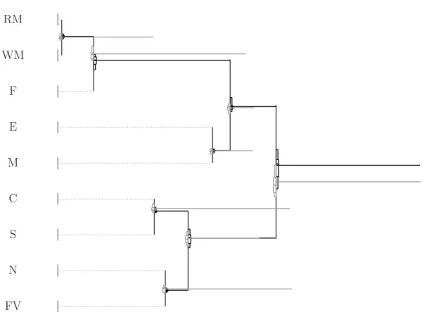
A graphical representation of a sequential binary partition, together with additional statis-tical summaries of balances, constitutes a CoDa-dendrogram (Figure 1). Elements of the CoDa-dendrogram are (Egozcue and Pawlowsky-Glahn, 2005a, 2006; Pawlowsky-Glahn, Egozcue, and Tolosana-Delgado, 2007; Thi´o-Henestrosa, Egozcue, Kov´acs, and Kov´acs, 2008):
1. The sequential binary partition represented by the dendrogram-type links between parts. The vertical bars describe the groups of parts formed at each order of parti-tion. The length of the vertical lines does not contain any quantitative information; they are as long as required to connect the parts in a group. Each one represents an interval(−u, u), whereuis user defined. That way, segments of different length can be intuitively compared, e.g. when a box-plot is located in the middle, or occupies a similar proportion of the segment.
2. The location of the mean of a balance, which is determined by the intersection of the vertical segment with the horizontal segment.
3. The decomposition of the sample total variance and the variability of each balance, represented by the length of the thick horizontal bars. The sum of all horizontal bars represents the total variance of the sample. A short horizontal bar means that the balance has a small variability in the sample, thus explaining only a little bit of the total variance. Conversely, a long horizontal bar implies a balance explaining a good deal of the total variance.
RM WM F E M C S N FV
Figure 1: CoDa-dendrogram. Bold = West; gray = East. Scale of vertical bars(−4,4). Horizontal scale is proportional to the total variance, which in this case is2.65Aitchison square-distance units. See text for a detailed description.
Optional additional elements are
1. Summary statistics of the empirical distribution of each balance represented as quantile box-plots (p0.05, Q1, Q2, Q3, p0.95) on the vertical(−u, u)intervals. The box-plot corresponding to one of the samples is located just above the segment, while the box-plot corresponding to the other sample is located below.
2. Several samples represented by overlapped CoDa-dendrograms, as shown in Figure 1, where the bold segments and box-plots correspond to western countries and the gray ones to eastern countries in Europe. To obtain an interpretable overlay, the most variable sample has to be plotted first.
The CoDa-dendrogram in Figure 1 shows the following:
• Balances that should be checked for their discrimination power using e.g. at-test are: b1 (animal/vegetal origin), b3 (meat/fish), and b7 (cereals/starch). The two groups of parts, G11 = {RM,WM,E,M,F}, and G12 = {C,S,N,FV}, are good candidates for discrimination, as the two means in balance b1 are well sep-arated and thus quite different, while the variances are very similar. The same arguments hold forb3, separatingG31 = {RM,WM} andG32 = {F}, while for
b7, with G71 = {C} andG72 = {S}, the variances are quite different. Note that the mean consumption of animal products compared to vegetal products is less in
the East than in the West, while the mean consumption of meat compared to fish is exactly the reverse. This is also the case for the mean consumption of cereals compared to starch, as shown by balanceb7.
• the means of the other balances are not informative, although in some cases there is a clear difference between the variances (see balancesb2,b4,b5, andb8);
• balance b6 (flours/other veg.) is very similar (in mean and variance) for east and west countries and does not give any information for discrimination.
6
Criteria to Define a Partition
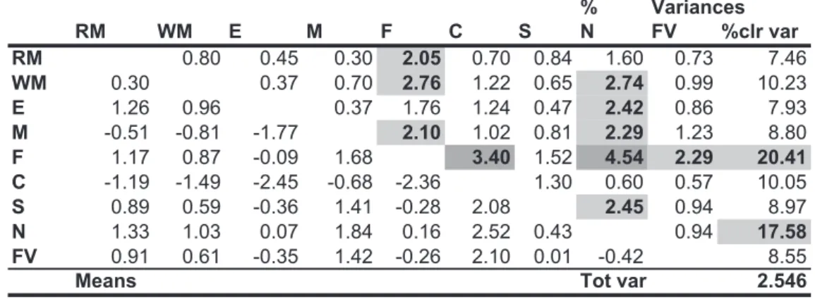
The intuitive approach presented above to define a partition is based on common sense. Usually, expert knowledge will be the essential tool for the approach. The question is what to do when there are no criteria on how to proceed. Two exploratory tools are very helpful for this purpose: (a) the variation array (Aitchison, 1986), shown in Figure 2; and (b), the biplot (Aitchison and Greenacre, 2002), shown in Figure 3 jointly for eastern and western countries. The variation array shows the pairwise log-ratio means and the percentage of total variance represented by pairwise log-ratio variances of the components. The highest values have been highlighted using a gray-shaded background and boldface characters, showing that the highest variability is related to the consumption of fish (F), followed by the consumption of nuts (N).
% Variances RM WM E M F C S N FV %clr var RM 0.80 0.45 0.30 2.05 0.70 0.84 1.60 0.73 7.46 WM 0.30 0.37 0.70 2.76 1.22 0.65 2.74 0.99 10.23 E 1.26 0.96 0.37 1.76 1.24 0.47 2.42 0.86 7.93 M -0.51 -0.81 -1.77 2.10 1.02 0.81 2.29 1.23 8.80 F 1.17 0.87 -0.09 1.68 3.40 1.52 4.54 2.29 20.41 C -1.19 -1.49 -2.45 -0.68 -2.36 1.30 0.60 0.57 10.05 S 0.89 0.59 -0.36 1.41 -0.28 2.08 2.45 0.94 8.97 N 1.33 1.03 0.07 1.84 0.16 2.52 0.43 0.94 17.58 FV 0.91 0.61 -0.35 1.42 -0.26 2.10 0.01 -0.42 8.55
Means Tot var 2.546
Figure 2: % total variance, variation array. Upper triangle, pairwise log-ratio variances in percentage of total variance; lower triangle, pairwise log-ratio means.
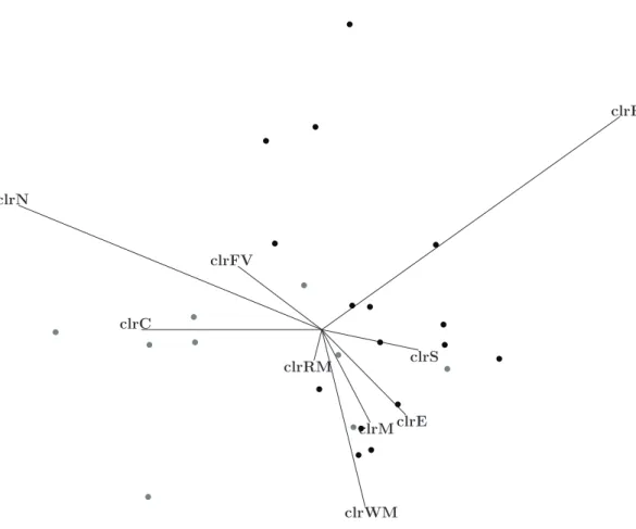
The compositional biplot is obtained as a standard covariance biplot for the centered log-ratio (clr) data. The clr transformation of compositional data (Aitchison, 1986) is given by clr(x) = log ( x1 g(x), x2 g(x), . . . , xD g(x) ) , g(x) = ( D ∏ j=1 xj )1/D ,
where the logarithm applies componentwise. In the biplot (Figure 3) the length of the rays is approximately proportional to the variance of the clr-components. We recognise theclr
clrRM clrWM clrE clrM clrF clrC clrS clrN clrFV • • • • • • • • • • • • • • • • • • • • • • • • •
Figure 3: Biplot. Black dots = West; gray dots = East. Length of rays are approximately proportional to the variance of theclr-transformed parts. Length of links between the end point of rays are approximately proportional to the corresponding variance of the pairwise log-ratio.
ofFand Nin the biplot easily, because they have the longest rays. We also see that the
clr-parts of animal origin point to the right (positive axis of the first principal component), while those of vegetal origin point to the left, exception made of clr of starch S. These facts, combined with the intuitive notions of nutrition, tell us, that the partition used in section 3 is probably quite discriminant between eastern and western countries (see also the distribution of these countries in the biplot).
The second principal axis confronts the clr of fish, F, fruits and vegetables,FV, and nuts,N, with the clr of meatsRMandWM, and eggsE, suggesting the so-called Mediter-ranean dietfor positive values of this second principal component. To analyse differences between northern and southern (Mediterranean) countries, the observation of the biplot might suggest a first partition into {C, S} versus {RM, WM, M, E, F, N, FV} and a second step {RM, WM, M, E}versus {F, N, FV}. The first balance would be of low discrimination power, while the second balance may discriminate quite well northern and Mediterranean countries. This shows that the use of compositional biplots, combined with expert knowledge, may help to define a sequential binary partition to get a meaningful set of balances and an interpretable dendrogram.
7
Conclusions
Balances are a special case of log-ratios with a particular interpretation due to their re-lationship with groups of parts. The CoDa-dendrogram uses the representation of com-positions by balances. It is a powerful descriptive tool, as it allows the simultaneous visualisation of an orthonormal basis of balancing elements, the induced decomposition of the total variance, the sample mean values, and some quantiles of the distribution. The CoDa-dendrogram is able to summarise sample information even when compositional vectors have a large number of parts. Balances can be selected by the user in order to improve interpretability of the results when some kind of affinity between parts isa pri-ori stated or desired. The groups of parts are the result of a sequential binary partition of the whole compositional vector. This process of partition may be difficult to describe for high-dimensional problems. The CoDa-dendrogram visualises this sequential binary partition as a binary clustering of parts, leading to a more intuitive representation. Two-sample CoDa-dendrograms can be used for a preliminary comparison of Two-sample balance means and variances. For mean comparisons between two samples, it can identify which balances have significant different means and which may be irrelevant. Representation of more than two samples is possible using different colours, but box-plots are only visual-ized in the two sample case.
Acknowledgements
This research has been supported by the Spanish Ministry of Education and Science under projects MTM2009-13272 and ‘Ingenio Mathematica (i-MATH)’ No. CSD2006-00032 (Consolider – Ingenio 2010), and by theAGAUR of theGeneralitat de Catalunyaunder project Ref: 2009SGR424. The authors thank R. Olea for fruitful discussions, which much helped to improve the paper.
References
Aitchison, J. (1986). The Statistical Analysis of Compositional Data. London: Chapman and Hall. (Reprinted 2003 with additional material by The Blackburn Press) Aitchison, J. (1997). The one-hour course in compositional data analysis or compositional
data analysis is simple. In V. Pawlowsky-Glahn (Ed.), Proceedings of IAMG’97 – The III Annual Conference of the International Association for Mathematical Geology(Vols. I, II and addendum, p. 3-35)). Barcelona: International Center for Numerical Methods in Engineering (CIMNE).
Aitchison, J., and Egozcue, J. J. (2005). Compositional data analysis: where are we and where should we be heading? Mathematical Geology,37, 829-850.
Aitchison, J., and Greenacre, M. (2002). Biplots for compositional data.
Barcel´o-Vidal, C., Mart´ın-Fern´andez, J. A., and Pawlowsky-Glahn, V. (2001). Mathe-matical foundations of compositional data analysis. In G. Ross (Ed.),Proceedings of IAMG’01 – the VII annual conference of the international association for math-ematical geology(p. 20). Cancun: Kansas Geological Survey.
Billheimer, D., Guttorp, P., and Fagan, W. (2001). Statistical interpretation of species composition. Journal of the American Statistical Association,96, 1205-1214. Egozcue, J. J. (2009). Reply to “On the Harker variation diagrams; . . . ” by J. A. Cort´es.
Mathematical Geosciences,41, 829-834.
Egozcue, J. J., and Pawlowsky-Glahn, V. (2005a). CoDa-dendrogram: a new exploratory tool. In G. Mateu-Figueras and C. Barcel´o-Vidal (Eds.), Compositional Data Analysis Workshop - CoDaWork’05, Proceedings. Girona: Universitat de Girona. (http://ima.udg.es/Activitats/CoDaWork05/)
Egozcue, J. J., and Pawlowsky-Glahn, V. (2005b). Groups of parts and their balances in compositional data analysis. Mathematical Geology,37, 795-828.
Egozcue, J. J., and Pawlowsky-Glahn, V. (2006). Exploring compositional data with the CoDa-dendrogram. In E. Pirard, A. Dassargues, and H. B. Havenith (Eds.), Pro-ceedings of IAMG’06 – The XI Annual Conference of the International Association for Mathematical Geology. Li`ege: University of Li`ege, Belgium, CD-ROM. Egozcue, J. J., Pawlowsky-Glahn, V., Mateu-Figueras, G., and Barcel´o-Vidal, C. (2003).
Isometric logratio transformations for compositional data analysis. Mathematical Geology,35, 279-300.
Kolmogorov, A. N., and Fomin, S. V. (1957). Elements of the Theory of Functions and Functional Analysis(Vols. I+II). Mineola, NY: Dover Publications, Inc.
Pawlowsky-Glahn, V. (2003). Statistical modelling on coordinates. In S. Thi´o-Henestrosa and A. Mart´ın-Fern´andez (Eds.),CoDaWork’03 – Proceedings.Girona: Universitat de Girona. (http://ima.udg.es/Activitats/CoDaWork03/)
Pawlowsky-Glahn, V., and Egozcue, J. J. (2001). Geometric approach to statistical analysis on the simplex. Stochastic Environmental Research and Risk Assessment (SERRA),15, 384-398.
Pawlowsky-Glahn, V., and Egozcue, J. J. (2002). BLU estimators and compositional data.
Mathematical Geology,34, 259-274.
Pawlowsky-Glahn, V., Egozcue, J. J., and Tolosana-Delgado, R. (2007). Lecture Notes on Compositional Data Analysis.
(http://hdl.handle.net/10256/297)
Pe˜na, D. (2002). An´alisis de datos multivariantes. Madrid: McGraw Hill.
Thi´o-Henestrosa, S., Egozcue, J. J., Kov´acs, V. P.-G. O., and Kov´acs, G. (2008). Balance-dendrogram. a new routine of CoDaPack. Computer and Geosciences, 34, 1682-1696.
Authors’ addresses: Vera Pawlowsky-Glahn
Department of Computer Science and Applied Mathematics University of Girona, Spain
Juan Jose Egozcue
Department of Applied Mathematics Technical University of Catalonia Barcelona, Spain