Doctoral Dissertations Student Theses and Dissertations
Summer 2017
Numerical investigation on nonlocal problems with the fractional
Numerical investigation on nonlocal problems with the fractional
Laplacian
Laplacian
Siwei DuoFollow this and additional works at: https://scholarsmine.mst.edu/doctoral_dissertations
Part of the Mathematics Commons Department: Mathematics and Statistics Department: Mathematics and Statistics Recommended Citation
Recommended Citation
Duo, Siwei, "Numerical investigation on nonlocal problems with the fractional Laplacian" (2017). Doctoral Dissertations. 2742.
https://scholarsmine.mst.edu/doctoral_dissertations/2742
This thesis is brought to you by Scholars' Mine, a service of the Missouri S&T Library and Learning Resources. This work is protected by U. S. Copyright Law. Unauthorized use including reproduction for redistribution requires the permission of the copyright holder. For more information, please contact [email protected].
by SIWEI DUO A DISSERTATION
Presented to the Graduate Faculty of the
MISSOURI UNIVERSITY OF SCIENCE AND TECHNOLOGY In Partial Fulfillment of the Requirements for the Degree
DOCTOR OF PHILOSOPHY in
MATHEMATICS 2017 Approved by
Dr. Yanzhi Zhang, Advisor Dr. Xiaoming He
Dr. Vy Khoi Le Dr. John R. Singler
SIWEI DUO All Rights Reserved
Nonlocal models have recently become a powerful tool for studying complex sys-tems with long-range interactions or memory effects, which cannot be described properly by the traditional differential equations. So far, different nonlocal (or fractional differential) models have been proposed, among which models with the fractional Laplacian have been well applied. The fractional Laplacian (−∆)α/2 represents the infinitesimal generator of
a symmetric α-stable Lévy process. It has been used to describe anomalous diffusion, turbulent flows, stochastic dynamics, finance, and many other phenomena. However, the nonlocality of the fractional Laplacian introduces considerable challenges in its mathemat-ical modeling, numermathemat-ical simulations, and mathematmathemat-ical analysis.
To advance the understanding of the fractional Laplacian, two novel and accurate finite difference methods – the weighted trapezoidal method and the weighted linear inter-polation method are developed for discretizing the fractional Laplacian. Numerical analysis is provided for the error estimates, and fast algorithms are developed for their efficient implementation. Compared to the current state-of-the-art methods, these two methods have higher accuracy but less computational complexity. As an application, the solution behaviors of the fractional Schrödinger equation are investigated to understand the non-local effects of the fractional Laplacian. First, the eigenvalues and eigenfunctions of the fractional Schrödinger equation in an infinite potential well are studied, and the results provide insights into an open problem in the fractional quantum mechanics. Second, three Fourier spectral methods are developed and compared in solving the fractional nonlinear Schrödinger equation (NLS), among which the SSFS method is more effective in the study of the plane wave dynamics. Sufficient conditions are provided to avoid the numerical instability of the SSFS method. In contrast to the standard NLS, the plane wave dynamics of the fractional NLS are more chaotic due to the long-range interactions.
ACKNOWLEDGMENTS
First and foremost, I would like to express my deepest gratitude to my Ph.D. advisor Dr. Yanzhi Zhang for introducing me to this exciting field of mathematics and for her dedicated help, encouragement, advice and continuous support throughout my Ph.D. It has been my honor to be her first Ph.D. student. Her enthusiasm, integral perspective on research and her mission for providing high-quality work, has made a deep impression on me. I appreciate all her contributions of time, guidance, and funding to make my Ph.D. experience productive and stimulating. I am really glad to be associated with a person like Dr. Yanzhi Zhang in my life.
Besides my advisor, I would like to thank my Ph.D. committee members, Dr. Vy Choi Le, Dr. Xiaoming He, Dr. John Singler and Dr. Thomas Vojta for their helpful comments on my thesis and career advice in general.
I wish to thank my officemates Sabrina Streipert, Gulsah Yeni and Jinyu Du, my roommate Xuejing Liu for their warmly support academically and personally.
Lastly, I would like to thank my family for all their love and encouragement. To my late father Yongshun Duo, who raised me with a love of science, helped me to realize my own potential and always believed in me and encouraged me to follow my dream. To my beloved mother Ruohong Liu, who is supporting me in all my pursuits and showing me that the key to life is enjoyment. My thanks also goes to Guodong Cui for all his love and patient whose faithful support and everlasting encouragement during the final stages of this Ph.D. is deeply appreciated.
Page
ABSTRACT . . . iii
ACKNOWLEDGMENTS . . . iv
LIST OF ILLUSTRATIONS . . . ix
LIST OF TABLES . . . xii
SECTION 1. INTRODUCTION. . . 1
1.1. OBJECTIVES AND OVERVIEW OF THIS DISSERTATION ... 4
2. DIRICHLET FRACTIONAL LAPLACIAN AND RELATED OPERATORS. . . 9
2.1. DIRICHLET FRACTIONAL LAPLACIAN ... 9
2.2. SPECTRAL FRACTIONAL LAPLACIAN ... 11
2.3. REGIONAL FRACTIONAL LAPLACIAN ... 12
2.4. PERIDYNAMIC OPERATOR ... 14
2.5. NUMERICAL COMPARISONS... 16
2.5.1. Nonlocal Effects of Operators ... 17
2.5.2. Eigenvalues and Eigenfunctions ... 22
3. THE WEIGHTED TRAPEZOIDAL METHOD IN 1D . . . 28
3.1. NUMERICAL SCHEME ... 28
3.2. ERROR ESTIMATES ... 33
4. THE WEIGHTED TRAPEZOIDAL METHOD IN HIGHER DIMENSIONS. . . 51
4.1. TWO-DIMENSIONAL CASE ... 51
4.1.1. Numerical Scheme ... 51
4.1.2. Error Estimates ... 57
4.1.3. Numerical Experiments ... 77
4.2. HIGHER DIMENSIONAL CASE ... 79
4.2.1. Numerical Scheme ... 79
4.2.2. Numerical Experiments ... 87
5. THE WEIGHTED LINEAR INTERPOLATION METHOD . . . 89
5.1. ONE-DIMENSIONAL CASE ... 89 5.1.1. Numerical Scheme ... 89 5.1.2. Error Estimates ... 92 5.1.3. Numerical Experiments ... 96 5.2. TWO-DIMENSIONAL CASE ... 99 5.2.1. Numerical Scheme ... 99 5.2.2. Numerical Experiments ... 101
6. COMPARISON OF NUMERICAL METHODS . . . 104
6.1. NUMERICAL METHODS ... 104
6.1.1. Interpolation Method ... 104
6.1.2. Finite Element Method ... 106
6.2. NUMERICAL COMPARISONS... 110
6.2.1. Discretization of the Fractional Laplacian ... 110
6.2.2. Solution of the Fractional Poisson Equation ... 113
7. THE FAST IMPLEMENTATION . . . 121
7.2. TWO-DIMENSIONAL CASE ... 123
7.3. THREE-DIMENSIONAL CASE... 126
8. THE FRACTIONAL SCHRÖDINGER EQUATION IN AN INFINITE POTEN-TIAL WELL. . . 132
8.1. STATIONARY STATES... 133
8.1.1. Standard Schrödinger Equation ... 134
8.1.2. Fractional Schrödinger Equation... 136
8.2. FRACTIONAL GRADIENT FLOW AND ITS DISCRETIZATION ... 139
8.3. FRACTIONAL LINEAR SCHRÖDINGER EQUATION... 142
8.3.1. Ground States ... 143
8.3.2. The First Excited States ... 146
8.4. FRACTIONAL NONLINEAR SCHRÖDINGER EQUATION ... 151
8.4.1. Ground States ... 152
8.4.2. The First Excited States ... 156
9. PLANE WAVE DYNAMICS OF THE FRACTIONAL SCHRÖDINGER EQUA-TION . . . 160
9.1. LINEAR STABILITY ANALYSIS ... 161
9.2. NUMERICAL METHODS ... 171
9.2.1. Split-step Fourier Spectral Method ... 172
9.2.2. Crank–Nicolson Fourier Spectral Method... 177
9.2.3. Relaxation Fourier Spectral Method... 180
9.2.4. Comparison in Simulating Plane Waves... 183
9.3. NUMERICAL INSTABILITY OF SSFS ... 188
9.4. NUMERICAL STUDY ON PLANE WAVE DYNAMICS ... 195
9.4.1. Focusing NLS... 195
10. CONCLUSION . . . 203 APPENDICES A. DERIVATION OF REMARK 9.3.2 . . . 206 B. DERIVATION OF REMARK 9.3.3 . . . 209 REFERENCES . . . 211 VITA . . . 220
Figure Page
2.1 Comparison ofLuwithuin (2.11)... 18
2.2 Difference max|Lhu− Lpu|versus the horizon sizeδ for variousα, withu(x) defined in (2.11), ... 19
2.3 Comparison ofLuwithuin (2.12) andq= 2. ... 20
2.4 Comparison ofLuwithuin (2.12) andq= 2. ... 21
2.5 Comparison ofLuwithuin (2.12) andq= 1. ... 22
2.6 The absolute and relative differences in the eigenvalues of the fractional Lapla-cian and spectral fractional LaplaLapla-cian. ... 25
2.7 The first and second eigenfunctions of the spectral fractional Laplacian, frac-tional Laplacian, and regional fracfrac-tional Laplacian... 26
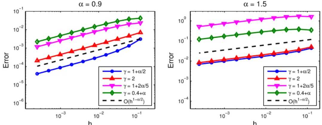
3.1 Numerical errors k(−∆)α/2u− (−∆)α/h,γ2uk∞,Ωfor different choices ofγ, where uis defined in (3.47) withs =1. ... 47
3.2 Convergence rate versusαforu∈C2,α/2(R)defined in (3.47) withs =2. ... 49
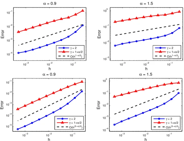
4.1 Numerical errors of the weighted trapezoidal method forγ =2 and 1+α/2 for udefined in (3.47) with s= 1. ... 78
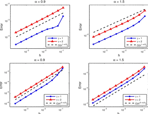
5.1 Numerical errors of the weighted linear interpolation method forγ = 1 and 2 for defined in (3.47) withs =1. ... 97
5.2 Numerical errors of the weighted linear interpolation method forγ = 1 and 2 withu ∈C1,α/2(R2) defined in (4.52) withs =1. ... 102
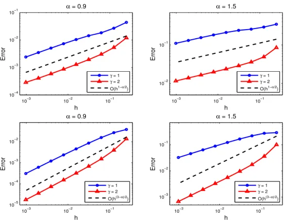
6.1 Bump function and numerical errors. ... 111
6.2 Comparison of numerical errors and rates. ... 114
6.3 Numerical errors in solving the fractional Poisson equation (6.17) by finite element method, weighted trapezoidal method, and linear interpolation method. 115 6.4 Relations between the convergence rates for solving the fractional Poisson equation and the fractional powerαinl∞-norm and inl2-norm. ... 116
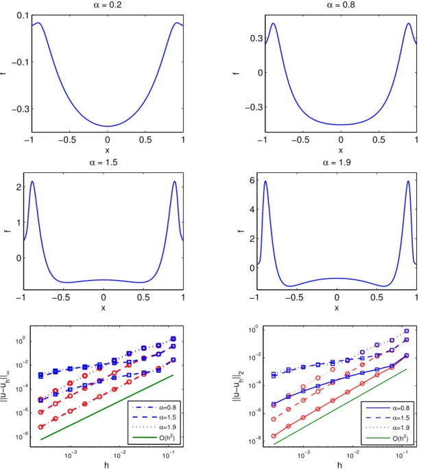
6.5 Numerical errors in solving the fractional Poisson problem (6.18) by finite element method, weighted trapezoidal method, and linear interpolation method forα= 0.4,1,1.5,1.9... 118
6.6 Relations between the convergence rates for solving the fractional Poisson
equation and the fractional powerαinl∞-norm and inl2-norm. ... 119
8.1 Ground states and expected value of position. ... 143
8.2 Comparison of the ground state solutions obtained from our method, Zoia’s method in [96], and Żaba’s method in [90] withV0 =100 andV0= 500. ... 145
8.3 Comparison of the ground state solutions and errors of eigenvalues. ... 145
8.4 The first excited state solutions and expected value of position. ... 147
8.5 The maximum value of the position density and the position. ... 148
8.6 Comparison of the first excited state solutions from our method, Zoia’s method in [96], and Żaba’s method in [90] withV0= 100 andV0=500. ... 149
8.7 Comparison of the first excited state solutions and the errors of the eigenvalues. 150 8.8 Ground state wave functions of the fractional nonlinear Schrödinger equation and the variance in position. ... 152
8.9 Log-log plots of the width of boundary layers versus β in the ground states of the fractional nonlinear Schrödinger equation in an infinite potential well. ... 154
8.10 Comparison of the ground states of the fractional nonlinear Schrödinger equa-tion in a finite potential well with depth V0 and those in an infinite potential well, where β = 10. The right panel is an enlarged display of the left panel around the maximum and boundary of the ground state solution. ... 155
8.11 The first excited state wave functions of the fractional nonlinear Schrödinger equation and the variance in position. ... 157
8.12 Comparison of the first excited states of the fractional nonlinear Schrödinger equation in a finite potential well with depthV0and those in an infinite potential well, where β =10. ... 158
9.1 Illustration of Theorem 9.1.2 (a). ... 166
9.2 Illustration of Theorem 9.1.2 (b)... 166
9.3 Contour plots of Re(Λl)for the plane wave solution (9.5) witha = 12... 169
9.4 Contour plots of Re(Λl)forγ <0. ... 170
9.5 Comparison of unstable modes forα= 0.9,1 and 1.1... 171
9.6 Time evolution of Re(u(0,t)) and Im(u(0,t)) from the exact solution (9.52), the SSFS method and the CNFS method. ... 185
9.7 Numerical errors in Re(u(0,t))and Im(u(0,t))of the SSFS and CNFS methods,
whereα=2 orα =1. ... 186 9.8 Illustration of the instability of SSFS. ... 188 9.9 Dynamics of the unstable plane wave solution in the 1D focusing NLS with
γ = −1 and λk =0 in the initial state (9.67). ... 196
9.10 Time evolution of the wave function around the peak first appears withγ = −1 in the fractional NLS (9.1) andλk =0 in the initial state (9.67). ... 197
9.11 Time evolution of log10|F(u(x,t))|in the 1D focusing NLS withγ = −1 and
λk = 0 in the initial condition (9.67). ... 198
9.12 Dynamics of the unstable plane wave solution in the 1D focusing NLS with
γ = −1 and λk =4π/L in the initial state (9.67). ... 199
9.13 Time evolution of the wave function around the time when the peak first appears withγ =−1 in the fractional NLS (9.1) andλk = 4π/Lon the initial state (9.67). 200
9.14 Time evolution of log10|F(u(x,t))|in the 1D focusing NLS withγ = −1 and
λk = 4π/L in the initial state (9.67). ... 201
9.15 Dynamics of the unstable plane wave solution in the 1D defocusing NLS with
LIST OF TABLES
Table Page
2.1 Comparison of the eigenvalues for different operators, where the eigenvalues of
the standard Dirichlet Laplace operator−∆are presented in most right column. . 23
3.1 Numerical errors and convergence rates foru ∈C1,α/2(R). ... 48
3.2 Numerical errors and convergence rates foru ∈C3,α/2(R). ... 49
4.1 Numerical errors of the fractional Laplacian foru ∈C3,α/2(R2). ... 79
4.2 Numerical errors of the fractional Laplacian foru ∈C3,α/2(R3). ... 87
5.1 Numerical errors by weighted interpolation method foru∈C3,α/2(R)withγ =1. 98 5.2 Numerical errors by weighted interpolation method foru∈C3,α/2(R)withγ =2. 98 5.3 Numerical errors by weighted linear interpolation method foru ∈C3,α/2(R2). ... 102
8.1 The eigenvalue µg of the ground states of the fractional linear (β = 0) Schrödinger equation in an infinite potential well. ... 147
8.2 The eigenvalue µ1 of the first excited states of the fractional linear (β = 0) Schrödinger equation in an infinite potential well. ... 151
8.3 The simulated eigenvalue µh gand the kinetic energy µhg,kinof the ground states of the fractional nonlinear Schrödinger equation in an infinite potential well. .... 155
8.4 The simulated eigenvalue µh 1 and the kinetic energy µ1h,kin of the first excited states of the fractional nonlinear Schrödinger equation in an infinite potential well. ... 158
9.1 MassN(t)by different methods. ... 184
In the last couple of decades, nonlocal or fractional differential models have become a powerful tool for modeling phenomena which cannot be described properly by the integer-order partial differential equations. Recent experiments in the study of diffusion processes which take places in various complex systems perform significant deviations from the standard laws of diffusion [21, 67]. Under such settings, the standard Laplacian∆which
processes a mathematical description of the normal diffusion fails to reproduce the observed anomalous diffusion behavior, and the fractional models have to take the place as an alternative modeling approach. So far, different fractional differential models have been proposed, among which models with the fractional Laplacian have been well applied in the field of the anomalous diffusion or dispersion [25, 30], turbulent flows [13, 76], porous media flows, quantum mechanics [33, 63], stochastic dynamics [40], finance [20], and many others.
Contrary to the standard Laplacian, the fractional Laplacian is a nonlocal operator defined on the entire space. Over Rd, the fractional Laplacian (−∆)α/2 is defined via a
pseudo-differential operator with symbol|ξ|α [62, 73]:
(−∆)α/2u(x) = F−1|ξ|αF[
u], for α >0, (1.1)
where F represents the Fourier transform, and F−1 is the inverse Fourier transform. In a special case withα = 2, the definition in (1.1) reduces to the standard Laplace operator −∆. The definition in (1.1) enables one to utilize the fast Fourier transform to efficiently
solve problems involving the fractional Laplacian, however, it is suitable only for problems defined either on the whole space Rd or on a bounded domain with periodic boundary
Laplacian(−∆)α/2is introduced [28, 62, 73, 80]: (−∆)α/2u(x) = Cd,α P.V. Z Rd u(x)−u(y) |y−x|d+α dy, for α∈ (0,2), (1.2)
where P.V. stands for the principal value, andCd,α is the normalization constant given by
Cd,α = 2
α−1αΓ (
d+α)/2 √
πdΓ 1−α/2 (1.3)
withΓ(·)denoting the Gamma function. From the probabilistic point of view, the fractional
Laplacian (−∆)α/2 represents the infinitesimal generator of a symmetric α-stable Lévy
process [3, 18]. In contrast to (1.1), the definition in (1.2) can easily incorporate with non-periodic bounded domains. Note that the integral representation in (1.2) is defined for 0< α <2, while the pseudo-differential definition in (1.1) is valid for allα >0. The equivalence of definitions (1.1) and (1.2) forα ∈ (0,2) are studied in [26, Proposition 3.3] and more
discussions can be found in [26, 60, 73, 88] and references therein. Recently, many studies have been carried out onthe Dirichlet fractional Laplacian, i.e., the fractional Laplacian on
a bounded domain with extended homogeneous Dirichlet boundary condition. However, the current understanding of this topic still remains limited, and the main challenges are from the approximation of the hypersingular integral combining with the non-local boundary condition. So far, numerical methods for directly discretizing the Dirichlet fractional Laplacian still remains limited.
The fractional Schrödinger equation was introduced by Laskin [63, 64] as a result of extending the Feynman path integral over Brownian trajectories to Lévy trajectories. It is a fundamental model of factional quantum mechanics that is expected to reveal some novel phenomena that are absent from its standard (non-fractional) counterpart. In [94], a zigzag propagation of light is found in the fractional Schrödinger equation with parabolic potential, which is different from the phenomena that is observed in the standard Schrödinger equation. Moreover, several optical realizations of the fractional Schrödinger equation have
been recently proposed in [65, 94, 95], and references therein. Although lots of topics under the context of the standard Schrödinger equation have been well studied, such as the infinite potential well model, the dynamics of the plane waves, due to the nonlocality arises from the fractional Laplacian, the studies of the fractional Schrödinger equation are still very limited.
The Schrödinger equation in an infinite potential well plays an important role in the understanding of the difference between the classical and quantum mechanics. To understand the difference between classical and fractional quantum mechanics, numerous studies have been devoted to finding the eigenvalues and eigenfunctions of the fractional Schrödinger equation in an infinite potential well [8, 27, 47, 48, 50, 59, 63, 66]. However, there is one continuing debate in the literature that whether the fractional linear Schrödinger equation in an infinite potential well has the same eigenfunctions as those of its standard (non-fractional) counterpart [8, 27, 47, 50, 66]. The analytical result still remains open and as conjectured in [66], that the eigenfunctions of the fractional Schrödinger equation cannot be written in terms of elementary functions. The difficulties arise not only in the analysis but also in its computations. So far, no study has been carried out by directly solving the fractional Schrödinger equation with an infinite potential well numerically.
In the study of the standard NLS equation, the plane wave solution is one of the most fundamental solution which plays important role in the study of many other more complex solutions. In the last couple of decades, the modulated plane wave dynamics attracted much attention in the study of NLS equation which has been experimentally confirmed with applications in the modulations of deep water waves [86]. The modulational instability (or the Benjamin–Feir instability) of the plane wave solutions has been well studied which mainly depends on the nonlinearity of the NLS. As shown in [86], the plane waves are always stable if the nonlinearity is defocusing; in contrast, they could have long-wave instability in the focusing case. Due to the conservation properties of the NLS, the unstable perturbations do not grow unboundedly, and thus the recurrence of the plane wave solution is observed
in the dynamics of the standard focusing NLS [89]. To numerically study the plane wave dynamics, numerical methods should be able to capture the analytical instability of the plane wave solutions without introducing numerical instability. Recently, many studies have been carried out to understand the instability in solving the plane wave solution by different numerical methods; see [12, 22, 37, 61, 70, 86] and references therein. Similar to the standard NLS, the fractional NLS conserves mass and energy, and admits the plane wave solution. However, the plane wave stability and their dynamics of the fractional NLS have not been studied in detail. In addition, only a few numerical methods are available in the literature for solving the fractional NLS. Both analysis and computations are desired to understand the plane wave stability and dynamics of the fractional NLS.
1.1. OBJECTIVES AND OVERVIEW OF THIS DISSERTATION
The objectives of this dissertation include: (i). The development of accurate and efficient numerical methods for directly discretizing the fractional Laplacian. (ii). The understanding of the solution properties of the fractional Schrödinger equations.
In Part I (Sections 2–7), we develop two novel finite difference methods for directly discretizing the fractional Laplacian and compare them with the exist numerical methods in the literature. Because of the challenges in approximating its hypersingular integral, so far numerical methods for discretizing the fractional Laplacian still remain limited. To avoid integrating the hypersingular integral (1.2) over the entire space, some other nonlocal operators that are closely related to the fractional Laplacian have been proposed in recent years, including the regional fractional Laplacian, the spectral fractional Laplacian, and the peridynamic operator. To understand the connections and differences among these nonlocal operators, in Section 2, we compare the properties of the fractional Laplacian with the other three nonlocal operators from various aspects. We show that on a bounded domain, the spectral fractional Laplacian and regional fractional Laplacian are significantly different from the Dirichlet fractional Laplacian, although they can be used to approximate each other
as the powerα →2. The peridynamic operator can provide a consistent approximation to the fractional Laplacian for anyα ∈ (0,2), but a large horizon size is required to obtain a
good approximation, especially whenαis small.
It is well known that the central finite difference scheme has the second order of accuracy for discretizing the standard Laplacian if the function is smooth enough. It arises a question that whether we can extend this idea to develop a corresponding second order scheme for the fractional Laplacian. In Sections 3–5, we develop two novel and accurate finite difference methods – the weighted trapezoidal method and the weighted linear interpolation method to directly discretize the fractional Laplacian (1.2). The key idea of both methods is to rewrite the hypersigular integral form of the fractional Laplacian as a weighted integral. By choosing proper weight functions, both of these two methods provide the second order of accuracy for smooth enough functions. We provide error analysis for the local truncation error of both methods in one and two-dimensions. The proof in higher dimensions can follow the same idea as in two-dimensional cases. The main technique used in the analysis of the weighted trapezoidal method is the weighted Montgomery’s identity, where its standard counterpart has been widely applied in the error analysis of the standard quadrature rules. The weighted trapezoidal method and the weighted linear interpolation method provide same convergence rates. In one dimension, the difference between their computational costs is insignificant, however, the weighted linear interpolation method has higher computational cost than the weighted trapezoidal method in higher dimensions. In contrast to the one-dimensional case where the single integrals can be evaluated exactly, in higher dimensions, the double/triple integrals can only be evaluated numerically. Due to the basis functions, more double/triple integrals appear in the weighted linear interpolation scheme, which is the main reason that results in higher computational cost in higher dimensions. Because these two methods provide same accuracy, we will use the weighted trapezoidal method as a representation to compare with other numerical methods in the literature.
The current state of the art for directly discretizing the fractional Laplacian is the finite difference method proposed in [49]. To solve the fractional Poisson’s equation with homogeneous Dirichlet boundary condition, a finite element method is proposed in [2, 25] recently. In Section 6, we compare our weighted trapezoidal method as a representation with the scheme proposed in [49] for discretizing the fractional Laplacian. We also compare theses two finite difference methods with the finite element method proposed in [2, 25] for solving the fractional Poisson’s equation and address the computational issues arising in the implementation of the finite element method. Our comparison results show that the weighted trapezoidal method has higher accuracy than the finite difference method in [49], moreover, its implementation is much simpler than the finite element method for solving the fractional Poisson’s equation.
In contrast to the standard Laplacian, the discretization of the fractional Laplacian results in a large dense matrix A due to its nonlocality. A direct computation of the matrix-vector product Au has large computational costs, especially in higher dimensions.
In Section 7, we introduce a fast algorithm for computing the matrix-vector product Auof
the discretized fractional Laplacian with a vector-valued function. In fact, the discretized fractional Laplacian is a symmetric Toeplitz matrix whose structure can be exploited through the use of fast algorithms [15, 81, 84], and its computation can be achieved efficiently by using the fast Fourier transform (FFT). In addition, this fast algorithm can be directly extended to higher dimensions.
In Part II (Sections 8 and 9), as the applications of the fractional Laplacian, we study the solution properties of the fractional Schrödinger equation. In Section 8, we numerically study the ground and the first excited states of the fractional Schrödinger equation in an infinite potential well. The study of its eigenvalues and eigenfunctions has attracted massive attention from both physicists and mathematicians. There is a continuing debate in the literature that whether the fractional linear Schrödinger equation in an infinite potential well has the same eigenfunctions as those of its standard (nonfractional) counterpart. By
introducing a normalized fractional gradient flow combine with the weighted trapezoidal method, we numerically solve the eigenvalue problem of the fractional Schrödinger equation. Our numerical results suggest that the eigenfunctions of the fractional Schrödinger equation differ from those of the standard Schröodinger equations.
In Section 9, we study the modulational stability of the plane waves and their dynamics of the fractional nonlinear Schrödinger equation (NLS) both analytically and numerically. Firstly, we present the linear stability analysis of the plane wave solution and find that the stability in the fractional NLS is more complicated than that in the standard NLS. In contrast to the standard NLS, the plane waves are no longer always stable in the defocusing fractional NLS, the instability appears for the fractional powerα ∈(0,1]. Besides the linear
stability analysis, numerical simulation is a powerful tool to further understand the plane wave dynamics from its nonlinear stage. Since the plane wave solutions are studied, the periodic boundary condition is naturally associated with the fractional NLS. Thus, we adopt the pseudo-differential definition of the the fractional Laplacian (−∆)α/2 in (1.1), which
enables us to utilize the fast Fourier transform to efficiently solve the problem. We develop three Fourier spectral methods i.e., the split-step Fourier spectral (SSFS) method, the Crank-Nicolson Fourier spectral (CNFS), and the relaxation Fourier spectral (ReFS) method, for solving the fractional NLS. Our results suggest that the SSFS method is more efficient for studying the long-time behaviors of the plane wave solutions of the fractional NLS, since it preserves the dispersion relation. The plane wave dynamics of the fractional NLS are numerically studied by the SSFS method, and it suggests different phenomena from that in standard Schrödinger equation, such as the disappearance of the well-known recurrence of the plane wave solution forα , 2 and the leakage of the low-frequency instability to high frequency. The fractional power α represents the strength of the long-range interactions, the smaller the the fractional power, the stronger the long-range interactions, and more
chaotic the dynamics of the fractional NLS. Since the numerical simulation by SSFS method introduces instabilities that have no analytical counterpart, we provided sufficient conditions for the mesh size and time step to avoid such numerical instabilities.
In contrast to the entire space, the fractional Laplacian (1.2) on a bounded domain associated with the Dirichlet boundary condition (the Dirichlet fractional Laplacian) is of great interest, not only from the mathematical point of view, but also in practical appli-cations. Any equation involving the Dirichlet fractional Laplacian has to be enclosed by a nonconventional, nonlocal boundary condition imposed on the complement of the phys-ical domain where the governing equation is defined. Besides the hypersingularity from the fractional Laplacian (1.2), the nonlocal boundary condition also introduces significant challenge, especially in the numerical simulations. To avoid evaluation and analysis over the entire space, one common approach is to “truncate" and approximate the integral of the
Dirichlet fractional Laplacian. Therefore, some other nonlocal operators that are closely related to the Dirichlet fractional Laplacian have been proposed in recent years, including the regional fractional Laplacian, the spectral fractional Laplacian, and the peridynamic operator. In this section, we study and compare the properties of the Dirichlet fractional Laplacian with the other three related nonlocal operators. Our main purpose to understand the connections and differences among these nonlocal operators. LetΩ ⊂ Rd denote an open bounded domain, andΩc =Rd\Ωrepresents the complement ofΩ.
2.1. DIRICHLET FRACTIONAL LAPLACIAN
Recently, many studies have been carried out onthe Dirichlet fractional Laplacian
(also known as the restricted fractional Laplacian), i.e., the fractional Laplacian on a
bounded domain Ω with extended homogeneous Dirichlet boundary condition (u(x) ≡ 0 forx ∈Ωc). However, the current understanding of this topic still remains limited, and the
main challenge is from the non-locality of the operator. In the following, we will discuss some fundamental properties of the Dirichlet fractional Laplacian.
Probablisticly, the Dirichlet fractional Laplacian(−∆)α/2represents the infinitesimal
generator of a symmetricα-stable Lévy process that particles are killed upon leaving the domain Ω [18, 79, 88]. One fundamental issue in the study of the Dirichlet fractional
Laplacian is its eigenvalues and eigenfunctions. So far, their exact results still remain unknown, and only some estimates and approximations can be found in the literature. It shows in [17] that on a convex domainΩ ⊂ Rd, thek-th eigenvalue λk (for k ∈ N) of the
Dirichlet fractional Laplacian(−∆)α/2are bounded by [17]:
1 2µ α/2 k ≤ λk ≤ µ α/2 k , for α ∈ (0,2), (2.1)
where µk represents thek-th eigenvalue of the Dirichlet standard Laplace operator −∆on
the same domainΩ. That is, the eigenvalue of the fractional Laplacian is always smaller
than that of the standard Laplacian −∆. If a one-dimensional (i.e., d = 1) domain is
considered, the estimates in (2.1) can be improved, and sharper bounds can be found for two special cases, such ask = 1 andα ∈ (0,2) in [3, 35], andα= 1 andk = 1,2,3 in [3].
More discussion on the eigenvalue bounds can be found in [39, 51, 87, 88] and references therein. Furthermore, in a one-dimensional interval(−1,1), the asymptotic approximation
of the eigenvalueλk is given by [59]:
λk = kπ 2 − (2−α)π 8 !α +O 2−α k√α ! , for k ∈N. (2.2)
It further shows that ifα≥ 1, the eigenvalueλk(fork ∈N) is simple, and the corresponding
eigenfunction satisfies ϕk(−x) = (−1)k−1ϕ(x). Compared to the studies on eigenvalues,
the understanding of eigenfunctions is even less. It shows in [75] that the eigenfunction
ϕk (for k ∈ N) are Hölder continuous up to the boundary of a smooth bounded domain
Ω ⊂ Rd. Recent numerical results on eigenvalues and eigenfunctions of the Dirichlet fractional Laplacian can be found in [32, 33].
The fractional Poisson equation is one main building block in the study of fractional PDEs, which takes the following form [2, 25, 31, 35]:
(−∆)α/2u(x) = f(x), for x∈Ω, (2.3)
u(x)= 0, for x∈Ωc. (2.4)
In (2.4), the extended homogeneous boundary conditions are imposed onΩc,
distinguish-ing from the classical Poisson problem where boundary conditions are added on∂Ω. This
difference can be explained from probabilistic interpretation of the standard and fractional Laplacian. The standard Laplace operator represents the infinitesimal generator of a Brow-nian motion with continuous sample paths; thus for a particle in domainΩ, it must leave
the domain via the boundary points on ∂Ω. By contrast, the fractional Laplacian is the
infinitesimal generator of a symmetric α-stable Lévy process with discontinuous sample paths; particles may “jump” out of the domain without touching any boundary points on
∂Ω. Hence, the solution on Ω can be determined by the values at ∂Ω in the context of
classical Poisson equations but not in the context of fractional Poisson equations.
2.2. SPECTRAL FRACTIONAL LAPLACIAN
Thespectral fractional Laplacian(also known as thefractional power of the Dirich-let Laplacian, or the“Navier” fractional Laplacian) is defined via the spectral
decomposi-tion of the standard Laplace operator [1, 69, 75], i.e.,
(−∆Ω)α/2u(x)= X
k∈N
ck µα/k 2ϕk(x), for α >0, (2.5)
where µk and ϕk are the k-th eigenvalue and normalized eigenfunction of the standard
Dirichlet Laplace operator −∆ on the domain Ω. From a probabilistic point of view, it
process that first kills Brownian motion in a bounded domainΩand then subordinates it via
aα/2-stable subordinator [78, 79]. Here, we include the domainΩin the notation(−∆Ω)α/2 to reflect this process and to distinguish it from the fractional Laplacian(−∆)α/2. Specially,
ifα= 2 the definition in (2.5) reduces to the standard Dirichlet Laplace operator−∆on the
domainΩ.
The spectral fractional Laplacian is a nonlocal operator, and it is often used in the analysis of (partial) differential equations. The eigenvalues and eigenfunctions of the spectral fractional Laplacian are clearly suggested from its definition in (2.5), that is, the k-th eigenvalue of (−∆Ω)α/2 is µα/k 2, and the corresponding eigenfunction is ϕk(x).
We remark that the spectral fractional Laplacian and the Dirichlet fractional Laplacian represent generators of different processes, which is also reflected by their eigenvalues and eigenfunctions. The eigenfunctions of the spectral fractional Laplacian are smooth up to the boundary as the boundary allows, while those of the Dirichlet fractional Laplacian are only Hölder continuous up to the boundary [75]. Additionally, it is easy to conclude from (2.1) that the k-th eigenvalue of the Dirichlet fractional Laplacian is always smaller than
that of the spectral fractional Laplacian, fork ∈N.
2.3. REGIONAL FRACTIONAL LAPLACIAN
Theregional fractional Laplacian (also known thecensored fractional Laplacian)
is defined as [10, 43, 45, 46]: (−∆)Ωα/2u(x) =Cd,αP.V. Z Ω u(x)−u(y) |y−x|d+α dy, for α ∈(0,2), (2.6)
with the constantCd,α defined in (1.3). In contrast to the fractional Laplacian, the regional
fractional Laplacian(−∆)Ωα/2represents the infinitesimal generator of a censored α-stable
process that is obtained from a symmetricα-stable Lévy process by restricting its measure toΩ[78]. If the domainΩ =Rd, the regional fractional Laplacian collapses to the fractional
Laplacian(−∆)α/2. To distinguish it from the fractional Laplacian(−∆)α/2, we include the
subscript ‘Ω’ in the operator(−∆)α/Ω2to indicate the restriction of theα-stable Lévy process
to the domainΩ.
The regional fractional Laplacian is different from the Dirichlet fractional Laplacian, although they are freely interchanged in some literature. In fact, a symmetric α-stable Lévy process killed upon leaving the domain Ω (represented by the Dirichlet fractional
Laplacian) is a subprocess of the censored α-stable process (represented by the regional fractional Laplacian) killing inside the domainΩ, i.e., the trajectories may be killed inside Ωthrough Feynman-Kac transform [79]. Moreover, we will illustrate their difference using
a simple example. Consider a one-dimensional interval Ω = (−l,l). Let u be a smooth
function satisfyingu(x) =0 forx ∈Ωc. Then the difference between the regional fractional
Laplacian and the Dirichlet fractional Laplacian can be computed as:
Q1u(x) = (−∆)α/2−(−∆)Ωα/2u(x) = C1,α Z R u(x)−u(y) |x− y|1+α dy− Z l −l u(x)−u(y) |x−y|1+α dy ! = C1,α Z −l −∞ 1 |x−y|1+α dy+ Z ∞ l 1 |x−y|1+α dy ! u(x) = Cα1,α 1 (l+x)α + 1 (l− x)α ! u(x), for x ∈Ω. (2.7)
We find that in the limit case of α → 2, the difference between the regional fractional Laplacian and the Dirichlet fractional Laplacian vanishes, i.e.,Q1→ 0, due to the constant
C1,α → 0. In other words, the regional fractional Laplacian can be used to approximate the Dirichlet fractional Laplacian asα→ 2. While in the limit ofα→0, the difference in (2.7) reduces toQ1u→u, i.e., the Dirichlet fractional Laplacian can be written as the summation
of the regional fractional Laplacian and an identity operator. Otherwise, if α 0 and
α 2, the differenceQ1u ∼ O 1/(l− |x|)α, which does not tend to zero for any fixed
l,
In contrast to the fractional Laplacian, the current understanding on the regional fractional Laplacian still remains very limited. Recently, the interior regularity of the regional fractional Laplacian is discussed in [46, 68]. It shows that ifu ∈ Cp,s(Ω) for
s ∈ (α,1] oru ∈ Cp+1,s(Ω) for s ∈ (α−1,min(α,1)], then there is (−∆)Ωα/2u ∈ Cp(Ω),
wherep∈N. So far, no results of the eigenvalues or eigenfunctions on the regional fractional Laplacian can be found in the literature. Here, we expect that our numerical results could provide insights into the understanding of the properties of the regional fractional Laplacian in the future.
2.4. PERIDYNAMIC OPERATOR
The peridynamic models were originally proposed as a reformation of the classical solid mechanics in [77]. In contrast to the classical models, it properly accounts for the near-field nonlocal interactions so as to effectively model elasticity problems with discontinuity and other singularities. The general form of this nonlocal operator has the following form:
Lu(x) =
Z
B(x,δ)
K(x,y) u(x)−u(y)
dy, (2.8)
where B(x, δ) denotes a ball with its center at point x and radius δ, which represents the
interaction region of point x. The kernel function K(x,y) = K(|x− y|) describes the
interaction strength between pointsxandy. The constantδ >0 denotes the size of material
horizon, and in practical applications it is often chosen to be a small number.
Recently, the operator (2.8) with specially chosen kernel function is used to approx-imate the fractional Laplacian [25, 44]. We will refer it as theperidynamic operator and
denote it as (−∆)α/δ 2u(x)=Cd,α Z B(x,δ) u(x)−u(y) |x−y|d+α dy, (2.9)
i.e., the kernel function in this case is taken as: Kδ(x,y) = Cd,α |x−y|d+α, if y∈ B(x, δ), 0, otherwise.
In other words, Kδ(x,y) in the peridynamic operator represents a hard-threshold of the
kernel functionK(x,y)=Cd,α/|x−y|d+α of the fractional Laplacian, which can be viewed
as a truncation of K(x,y) in the fractional Laplacian. In the limit case of δ → ∞, the peridynamic operator (2.9) coincides with the fractional Laplacian (1.2), and thus it is often used to approximate the fractional Laplacian by choosing a sufficiently largeδ[25, 44]. On the other hand, note that the kernel functionK(x,y)has an algebraic decay of orderd+α,
which presents a heavy tail that accounts for considerable far field interactions. Hence, the cutoff of the kernel functionK(x,y) outside of the horizon B(x, δ) may have a significant
impact on its approximation to the fractional Laplacian as we shall show next.
Similarly, we choose a smooth function u satisfying u(x) = 0 for x ∈ Ωc with Ω = (−l,l) to illustrate the difference between the peridynamic operator and the Dirichlet
fractional Laplacian on a bounded domain. Here, we assume that the horizon sizeδin (2.9) is large enough, such that δ > max{l − x,l + x} for any point x ∈ (−l,l). Then, we can
compute their difference as:
Q2u(x) = (−∆)α/2−(−∆)δα/2u(x) = C1,α Z R u(x)−u(y) |x−y|1+α dy− Z x+δ x−δ u(x)−u(y) |x−y|1+α dy = C1,α Z x−δ −∞ 1 |x−y|1+α dy+ Z ∞ x+δ 1 |x−y|1+α dy ! u(x) = Cα1,α δ2αu(x), for x ∈Ω. (2.10)
It shows that the difference of these two operators is of order O(1/δα) when u(x) is
uniformly bounded onΩ, hence their difference vanishes asδ → ∞. On the other hand, the convergence of the peridynamic operator to the fractional Laplacian asδ→ ∞depends on the powerα, and it may degenerate rapidly for small α. Additionally, in the limit case of
α→2, the differenceQ2u→ 0, because the coefficientCd,α →0.
The peridynamic operator in (2.9) can be viewed as the infinitesimal generator of a symmtricα-stable process by restricting its measure toB(x, δ). In contrast to the regional
fractional Laplacian operator, the interaction region of pointxin the peridynamic operator
is symmetric with respect to itself. Hence, the peridynamic operator is expected to provide a symmetric approximation for a homogeneous elastic material.
In summary, the fractional Laplacian (1.2), spectral fractional Laplacian (2.5), regional fractional Laplacian (2.6), and the peridynamic operator (2.9) are all nonlocal operators in which every pointx interacts with other points yover certain long distance.
For a pointx∈Ω, the fractional Laplacian(−∆)α/2accounts for the interactions betweenx
andyfor ally ∈Rd\{x}. By contrast, the interaction region ofxin the regional fractional
Laplacian(−∆)Ωα/2is truncated toΩ\{x}, i.e., the same domain ofx, while the interaction
region of the peridynamic operator(−∆)δα/2reduces toB(x, δ)\{x}. We will further compare them in Section 2.5.
2.5. NUMERICAL COMPARISONS
In this section, we further compare these four nonlocal operators by studying their nonlocal effects, eigenvalues and eigenfunctions, and the solution behavior of the cor-responding nonlocal problems. In our simulations, the spectral fractional Laplacian is discretized by using the finite difference method combined with matrix transfer techniques introduced in [30], while the other three operators are discretized by the weighted trape-zoidal method developed in Section 3. Our numerical results provide insights not only to further understand these operators but also to improve the analytical results in the literature.
In the following, we will consider the one-dimensional cases. For notational simplic-ity, we will also useLhto represent the fractional Laplacian,Ls for the spectral fractional
Laplacian,Lr for the regional fractional Laplacian, andLpfor the peridynamic operator. 2.5.1. Nonlocal Effects of Operators. We compare the nonlocal effects of these
four operators by acting them on functions with compact support on the domainΩ = (−1,1). Example 1. Consider the function
u(x)= sinπ(1+x) 2 , if x ∈Ω, 0, otherwise, x ∈R, (2.11)
which is continuous on the whole spaceR. It is easy to obtain that
(−∆Ω)α/2u(x) = π 2 α sinπ(1+x) 2 , for x ∈Ω,
that is, the function from the spectral fractional Laplacian can be found exactly, while we will numerically compute the functions from the other three operators.
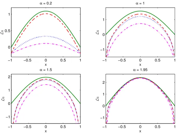
In Figure 2.1, we compare the functionLiufori = s, h, r, orp. The results clearly
suggest the difference between these four operators, especially the function Lsufrom the
spectral fractional Laplacian is significantly different from those of the other three operators. It shows that for anyα∈ (0,2), the functionLsuis proportional to the functionuon(−1,1).
In contrast, the properties ofLiu(fori = h,r, orp) significantly depend on the parameterα.
Forα ∈ (0,1), the functionLiuexists on the closed domainΩ, but they are very different
between operators. The smaller the parameterα, the larger the differences. Forα∈ [1,2),
the functionLiudoes not exist at the boundary points, i.e.,x = ±1. Asα→2, the function
−1 −0.5 0 0.5 1 0 0.5 1 x L u α = 0.2 −1 −0.5 0 0.5 1 −1 0 1 x L u α = 1 −1 −0.5 0 0.5 1 −1 0 1 2 x L u α = 1.5 −1 −0.5 0 0.5 1 −1 0 1 2 x L u α = 1.95
Figure 2.1. Comparison ofLuwithuin (2.11). The operatorLrepresentsLs (solid line),
Lh (dashed line),Lr (dashdot line), orLpwithδ = 4 (dotted line). Note that the plots in
y-direction are partially presented forα= 1, 1.5 or 1.95.
Additionally, Figure 2.1 shows that both the regional fractional Laplacian and peri-dynamic operator can be used to approximate the fractional Laplacian, if α is close to 2 (see Figure 2.1 forα = 1.95). For small α, the results from the regional fractional Lapla-cian are inconsistent with that from the fractional LaplaLapla-cian. However, the peridynamic operator can still provide a good approximation to the fractional Laplacian by enlarging the horizon sizeδ. Figure 2.2 presents the differences between the functionsLpuandLhufor
variousαandδ. It shows that for a fixed horizon sizeδ, the difference between these two operators dramatically decreases asαincreases. On the other hand, Figure 2.2 implies that for smallαthe convergence of the functionLputoLhucould be very slow. For instance,
100 101 102 103 104 10−8 10−6 10−4 10−2 100 δ max|(− ∆ ) α /2 u(x)−(− ∆ ) α /2 δ u(x)| α = 1.9 α = 1.5 α = 1.1 α = 0.6
Figure 2.2. Difference max|Lhu− Lpu|versus the horizon sizeδfor variousα, withu(x)
defined in (2.11),
for α = 0.6, the difference in Figure 2.2 is around 0.005 for a horizon size δ = 4000. In fact, the nonlocal interactions decay slowly for smallα, and thus a large horizon size δ is needed for the peridynamic operator to better approximate the fractional Laplacian.
Example 2. Consider the function
u(x)= (1−x2)q+α2, for x ∈Ω, 0, otherwise, x ∈R, (2.12)
forq∈N. For the fractional Laplacian, the analytical solution can be found as:
(−∆)α/2u(x) = 2 αΓ(α+1 2 )Γ(α2 +q+1) √ πΓ(q+1) 2F1 α+1 2 , −q; 1 2; x2 (2.13) forx ∈Ω, where2F1denotes the Gauss hypergeometric function. Moreover, we can obtain
the exact values of(−∆)Ωα/2uand(−∆)α/δ 2uby using their relation to the fractional Laplacian
in (2.7) and (2.10), respectively. For the spectral fractional Laplacian, we numerically computed(−∆Ω)α/2uby the finite difference method proposed in [30].
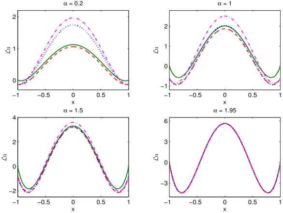
Figure 2.3 displays the function Liu for various α, where u is defined in (2.12)
with q = 2. It shows that the function Liu exists on the closed domain [−1,1] for any
α ∈ (0,2), but their values are very different, especially for small α. For the spectral
−1 −0.5 0 0.5 1 0 1 2 x L u α = 0.2 −1 −0.5 0 0.5 1 −1 0 1 2 x L u α = 1 −1 −0.5 0 0.5 1 −2 0 2 4 x L u α = 1.5 −1 −0.5 0 0.5 1 −3 0 3 6 x L u α = 1.95
Figure 2.3. Comparison ofLuwithuin (2.12) and q = 2. The operator L representsLs
(solid line),Lh(dashed line),Lr (dash-dot line), orLpwithδ= 4 (dotted line).
fractional Laplacian, the values of Lsu at the boundary are always zero, which inherits
from its definition in (2.5). For the regional fractional Laplacian, the functionuin (2.12)
withq = 2 satisfies the conditions thatu ∈ C2([−1,1]) andu0(±1) = 0, which guarantee
the existence of the function Lru for any α ∈ (0,2) [46]. Since the function u(±1) = 0
and the relations in (2.7) and (2.10), the values of Liu (fori = h,r and p) are the same
at boundary points, but they are nonzero. Figure 2.3 also shows that both the regional fractional Laplacian and the peridynamic operator with relatively smallδ could provide a good approximation to the fractional Laplacian, ifαis large (see Figure 2.3 forα =1.95).
Whileα is small, although the peridynamic operator can be still used to approximate the fractional Laplacian with a large δ, the regional fractional Laplacian is inconsistent with the fractional Laplacian.
Figure 2.3 additionally shows that as α → 2, the differences between the four operators become insignificant (see Figure 2.3 for α = 1.95), and the function Liu (for
i = h, s, r, or p) converges to−∂x xu, that is, the four operators converge to the standard
Dirichlet Laplace operator −∆. In contrast to cases of α → 2, the functions Lhu from
the fractional Laplacian and Lsu from the spectral fractional Laplacian converge tou, as
α → 0, while Lrufrom the regional fractional Laplacian and Lpu from the peridynamic
operator converge to a zero function; see Figure 2.4.
−1 −0.5 0 0.5 1 0 0.5 1 x L u α = 0.001
Figure 2.4. Comparison ofLuwithuin (2.12) and q = 2. The operator L representsLs
(solid line),Lh(dashed line),Lr (dash-dot line), orLpwithδ= 4 (dotted line).
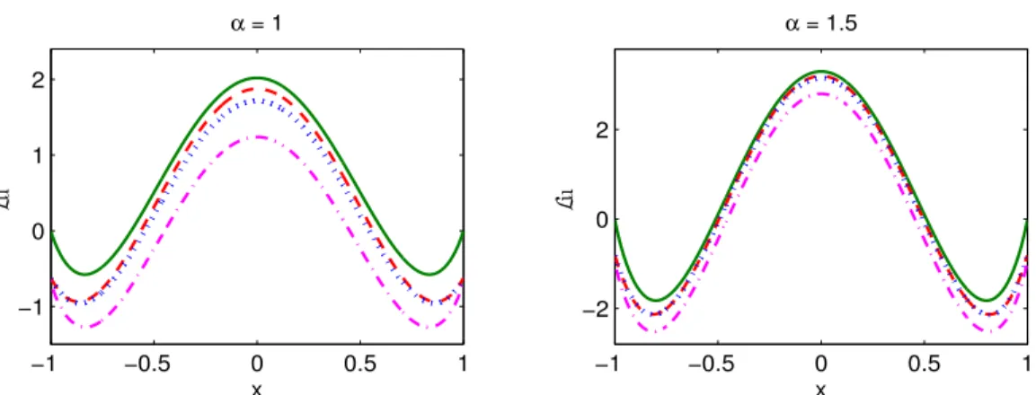
Moreover, our numerical results suggested that for α ∈ [1,2), if the functionu ∈
C1,α/2(Ω) and u0(±1) = 0, then the regional fractional Laplacian Lru exists; see Figure
2.5. Hence, we conjugate that the regularity results in [46] might be able to improve to
u ∈ C1,α/2(Ω)at least for one-dimensional case. More analysis needs to be carried out for
−1 −0.5 0 0.5 1 −1 0 1 2 x L u α = 1 −1 −0.5 0 0.5 1 −2 0 2 x L u α = 1.5
Figure 2.5. Comparison ofLuwithuin (2.12) and q = 1. The operator L representsLs
(solid line),Lh(dashed line),Lr (dash-dot line), orLpwithδ= 4 (dotted line).
2.5.2. Eigenvalues and Eigenfunctions. In this section, we compare the four
non-local operators by studying their eigenvalues and eigenfunctions on a one-dimensional bounded domainΩ= (−l, l).
Denoteλi kandφ
i
kas thek-th (fork ∈N) eigenvalue and eigenfunction of the
nonlo-cal operatorLi onΩwith the corresponding homogeneous Dirichlet boundary conditions,
wherei = h, s, r, or p. It is well known that the eigenvalues and eigenfunctions of the
spectral fractional LaplacianLs can be found analytically, i.e.,
λs k = µ α/2 k = kπ 2l !α/2 , φs k(x) = r 1 l sin kπ 2 1+ x l , x ∈ (−l,l),
fork ∈N. For the other operators, so far no analytical results can be found in the literature, and thus we will compute their eigenvalues and eigenfunctions numerically.
Table 2.1. Compar ison of the eig en values for different operators, where the eig en values of the standard Dir ic hlet Laplace operator − ∆ are presented in mos tr ight column. For eac h k ,upper ro w : λ s ;middle k ro w : λ h ;lo k w er ro w : λ r . k k α 0.2 0.5 0.7 0.9 1 1.2 1.5 1. 8 1.95 1.999 1 1.0945 1.2533 1.3718 1.5014 1.5708 1.7193 1.9687 2.2543 2.4123 2.4663 2.4674 0.9575 0.9702 1.0203 1.1032 1.1578 1.2971 1.5976 2.0488 2.3520 2.4650 0.0003 0.0038 0.0170 0.0640 0.1135 0.2939 0.8088 1.6602 2.2444 2.4628 2 1.2573 1.7725 2.2285 2.8018 3.1416 3.9498 5.5683 7.8500 9.3206 9.8583 9.8696 1.1966 1.6016 1.9733 2.4583 2.7549 3.4870 5.0600 7.5033 9.2082 9.8559 0.1878 0.4593 0.6729 0.9799 1.2026 1.8719 3.6509 6.7378 8.9854 9.8512 3 1.3635 2.1708 2.9598 4.0357 4.7124 6.4252 10.230 16.287 20.550 22.172 22.207 1.3191 2.0289 2.7294 3.6987 4.3171 5.9121 9.5948 15.800 20.384 22.169 0.3085 0.8626 1.3646 2.0823 2.5760 3.9902 7.7500 14.701 20.049 22.161 4 1.4442 2.5066 3.6201 5.2283 6.2832 9.0744 15.750 27.335 36.012 39.406 29.478 1.4106 2.3873 3.4131 4.9055 5.8925 8.5350 15.020 26.725 35.794 39.401 0.3981 1.2091 2.0140 3.2054 4.0292 6.3902 12.811 25.313 35.349 39.391 5 1.5101 2.8025 4.2322 6.3912 7.8540 11.861 22.011 40.847 55.645 61.558 61.685 1.4817 2.6949 4.0371 6.0733 7.4607 11.293 21.191 40.115 55.374 61.552 0.4700 1.5149 2.6231 4.3230 5.5171 8.9817 18.670 38.408 54.820 61.540 8 1.6590 3.5449 5.8809 9.7564 12.566 20.847 44.547 95.187 139.14 157.51 157.91 1.6400 3.4612 5.7133 9.4550 12.175 20.225 43.509 94.122 138.72 157.50 0.6296 2.2799 4.2751 7.6101 10.072 17.552 40.218 91.591 137.85 157.49 10 1.7347 3.9633 6.8752 11.926 15.708 27.249 62.256 142.24 215.00 246.06 246.74 1.7189 3.8886 6.7186 11.632 15.317 26.598 61.096 140.96 214.48 246.05 0.7095 2.7090 5.2735 9.7490 13.145 23.749 57.377 137.92 213.39 246.02 20 1.9926 5.6050 11.169 22.255 31.416 62.601 176.09 495.30 830.70 983.56 986.96 1.9836 5.5525 11.042 21.981 31.025 61.854 174.45 493.09 829.69 983.53 0.9779 4.3810 9.5850 19.998 28.657 58.439 169.09 487.74 827.58 983.49
In Table 2.1, we present the eigenvalues of the fractional Laplacian Lh, spectral
fractional LaplacianLs, and regional fractional LaplacianLr, on the domainΩ = (−1,1).
We leave the peridynamic operator Lp out of our comparison here, since its spectrum
depends on the horizon sizeδ. The eigenvalues of the standard Dirichlet Laplace operator −∆are presented in most right column in Table 2.1. For eachk, the upper row represents λs
k; the middle row representsλ h
k; the lower row represents λ r k.
From Table 2.1 and our extensive numerical studies, we find
λr k < λ h k < λ s k, for α ∈(0,2) and k ∈N,
that is, the eigenvalues of the regional fractional Laplacian are much smaller than those of the fractional Laplacian and spectral fractional Laplacian. However, as α → 2 the eigenvalue λi
k of these three operators converges to µk = k2π2/4 – the kth eigenvalue of
the standard Dirichlet Laplace operator−∆on(−1,1).
In [75], it is proved that the first eigenvalue of the fractional Laplacian is strictly smaller than that of the spectral fractional Laplacian, i.e., λh
1 < λs1, for α ∈ (0,2). Our
numerical results in Table 2.1 confirm this conclusion and additionally suggest that the eigenvalue λh
k is strictly smaller than λ s
k, for any k ∈ N. Furthermore, we present the
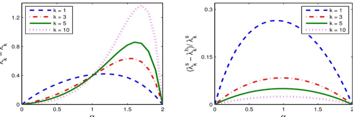
difference between the eigenvalues λs k and λ
h
k for variousα andk in Figure 2.6. It shows
that the difference between the eigenvalues λs k and λ
h
k depends on both parameters α and
k. For a given k ∈ N, there exists a critical valueαk where the gap betweenλsk and λhk is
maximized. The value ofαk increases ask ∈Nincrease (see Figure 2.6 left). On the other
hand, ask ∈N, the relative difference between the eigenvaluesλsk andλhkdecreases quickly (see Figure 2.6 right).
In Figure 2.7, we compare the first and second eigenfunctions of the fractional Laplacian, the spectral fractional Laplacian, and the regional fractional Laplacian. For any α ∈ (0,2), the eigenfunctions for these three operators are all symmetric (for odd
0 0.5 1 1.5 2 0 0.4 0.8 1.2 α λ k s − λ k h k = 1 k = 3 k = 5 k = 10 0 0.5 1 1.5 2 0 0.15 0.3 α ( λ k s − λ k h )/ λ k s k = 1 k = 3 k = 5 k = 10
Figure 2.6. The absolute (left panel) and relative (right panel) differences in the eigenvalues of the fractional Laplacian and spectral fractional Laplacian.
k) or antisymmetric (for even k) with respect to the center of the domain Ω. Especially,
the eigenfunctions of the spectral fractional Laplacian are independent of the parameter
α, which are also the eigenfunctions of the standard Dirichlet Laplace operator −∆. In
contrast, the eigenfunctions of the other two operators significantly depend on α, and as
α → 2, they converge to sin(kπ(1+ x)/2) – the eigenfunctions of the standard Dirichlet
Laplace operator−∆. Our numerical observations in Figure 2.7 justify the regularity results
in [75, Theorem 1], that is, the eigenfunctions of the fractional Laplacian is no better than Hölder continuous up to the boundary, while the eigenfunctions of the spectral fractional Laplacian are smooth up to the boundary as the boundary allows.
From our extensive studies, we find that the eigenvalues of the fractional Laplacian Lh, the spectral fractional LaplacianLs, and the regional fractional Laplacian Lr reduces
as the domain size increases. In particular, if the domain size increases by a ratio of κ, the k-th (for k ∈ N) eigenvalues decreases by a ratio of κα. Additionally, we explore the eigenvalues of the peridynamic operators for differentδ. It shows that the eigenvalue increases asδdecreases.
−1 −0.5 0 0.5 1 0 0.5 1 x φ 1 (x) α = 0.6 −1 −0.5 0 0.5 1 −1 0 1 x φ 2 (x) α = 0.6 −1 −0.5 0 0.5 1 0 0.5 1 x φ 1 (x) α = 1 −1 −0.5 0 0.5 1 −1 0 1 x φ 2 (x) α = 1 −1 −0.5 0 0.5 1 0 0.5 1 x φ 1 (x) α = 1.9 −1 −0.5 0 0.5 1 −1 0 1 x φ 2 (x) α = 1.9
Figure 2.7. The first (left panel) and second (right panel) eigenfunctions of the spectral fractional Laplacian (solid line), fractional Laplacian (dash-dot line), and regional fractional Laplacian (dashed line). Note that the eigenfunctions of the spectral fractional Laplacian are independent ofα >0.
In this section, we compare the properties of the Dirichlet fractional Laplacian with some related nonlocal operators, i.e., the spectral fractional Laplacian, the regional fractional Laplacian, and the peridynamic operator. Our study shows that their differences are significant on a bounded domain. Probabilistically, they represent the generators of different stochastic processes. In addition, the eigenvalues and eigenfunctions of these
four operators are different, although they all converge to those of the classical Laplace operator as α → 2. In conclusion, our extensive numerical investigations suggest that these three nonlocal operators can only serve as good approximations of the Dirichlet fractional Laplacian under some special situations but the deviations could be large as the fractional power α is relatively small. As α → 2, all the four operators collapse to the classical Dirichlet Laplacian. For relatively smallα, to provide a good approximation of the Dirichlet fractional Laplacian, the horizon size δ of the peridynamic operator must be taken sufficiently large; differently, the regional fractional Laplacian generally provides inconsistent results from the fractional Laplacian.
3. THE WEIGHTED TRAPEZOIDAL METHOD IN 1D
The traditional trapezoidal method is widely used in the field of numerical integra-tion, and it has the second order of accuracy if the integrand function is smooth enough. However, the fractional Laplacian defined in (1.2) is a hypersingular integral, and directly applying the traditional trapezoidal method fails to provide the optimal accuracy or to be convergent. It is known that the weighted quadrature rules are advantageous in approxi-mating the hypersingular integrals [23, Chapter 5]. By introducing a weight function, the hypersingular integral is formulated as a weighted integral of a weaker singular function.
In this section, we will develop a novel finite difference method based on the weighted trapezoidal rule to discretize the fractional Laplacian (1.2) in one dimension (1D). The error analysis will be provided for functions with different smoothness conditions. Some numerical examples are presented to justify the analytical results.
3.1. NUMERICAL SCHEME
Consider the fractional Laplacian defined in (1.2). We focus on the discretization of the fractional Laplacian on a one-dimensional bounded domainΩ with homogeneous
Dirichlet boundary conditions, i.e.,u(x) ≡ 0 forx ∈Ωc. Our scheme can be also used for
nonhomogeneous constant boundary conditions, i.e.,u(x)= gwithga constant forx ∈Ωc.
In this case, one can definev =u−g, and there is(−∆)α/2v = (−∆)α/2u.
Lettingξ = |x−y|, we can rewrite the one-dimensional fractional Laplacian in (1.2) as (−∆)α/2u(x) =−C1,α Z ∞ 0 u(x−ξ)−2u(x)+u(x+ξ) ξ1+α dξ. (3.1)
Define domainΩ = (a,b), and choose a constant L = |Ω| = b−a. We further write the integral in (3.1) as: (−∆)α/2u(x) = −C1,α Z L 0 u(x−ξ)−2u(x)+u(x+ξ) ξ1+α dξ + Z ∞ L u(x−ξ)−2u(x)+u(x+ξ) ξ1+α dξ . (3.2)
Note that for anyx ∈ (a, b)and ξ ≥ L, there is (x± ξ) ∈R\(a, b), and thus the function
u(x±ξ)≡ 0. Hence, the second integral in (3.2) reduces to
Z ∞ L u(x−ξ)−2u(x)+u(x+ξ) ξ1+α dξ =−2u(x Z ∞ L 1 ξ1+αdξ =− 2 αLαu(x), (3.3)
that is, it can be computed exactly.
Now, we will approximate the first integral in (3.2) numerically. Choose a positive integer N, and define the mesh sizeh = L/N. Denote grid pointsξi = ih, for 0 ≤ i ≤ N;
evidentlyξN = L. First, we introduce a splitting parameterγ ∈ (α,2]. The choice of γ is
important in determining the accuracy of our method, and we will carry out more discussion later. Then, we can formulate the first integral in (3.2) as:
Z L 0 u(x−ξ)−2u(x)+u(x+ξ) ξ1+α dξ = Z L 0 ψγ(x, ξ)ξ γ−(1+α)dξ = N X i=1 Z ξi ξi−1 ψγ(x, ξ)ξγ−(1+α)dξ, (3.4)
where for notational simplicity we define the function
ψγ(x, ξ)= u(x−ξ)−2u(x)+u(x+ξ)
That is, the first integral in (3.2) can be viewed as an weighted integral ofψγ, withξγ−(1+α) representing the weight function. For 2 ≤ i ≤ N, we use the weighted trapezoidal rule to
approximate the integrals in (3.4), i.e., Z ξi ξi−1 ψγ(x, ξ)ξγ−(1+α)dξ ≈ 1 2 ψγ(x, ξi−1)+ψγ(x, ξi) Z ξi ξi−1 ξγ−(1+α) dξ = 2 1 (γ−α) ξγ−α i −ξ γ−α i−1 ψγ(x, ξi−1)+ψγ(x, ξi) , (3.6)
for anyγ = (α,2]. While fori = 1, we will divide our discussion into two cases based on
different choice of the splitting parameter, i.e.,γ ∈ (α,2)orγ =2.
Case 1. The splitting parameterγ ∈ (α,2). Fori = 1, we can approximate the integral
as Z ξ1 ξ0 ψγ(x, ξ)ξ γ−(1+α)dξ ≈ 1 2(γ−α)ξ γ−α 1 ψγ(x, ξ1), (3.7)
which can be formally obtained using the weighted trapezoidal rule, i.e., Z ξ1 ξ0 ψγ(x, ξ)ξ γ−(1+α)dξ ≈ 1 2 lim ξ→0ψγ(x, ξ)+ψγ(x, ξ1) Z h 0 ξ γ−(1+α)dξ.
Assuming thatuis smooth enough, the above limit is zero, i.e.,
lim
ξ→0ψγ(x, ξ) ≈ ξlim→0ξ
2−γ
u00(x) =0.
Combining (3.2)–(3.4) and (3.6)–(3.7), we obtain the numerical approximation of the fractional Laplacian(−∆)α/2as:
(−∆)α/h,γ2u(x) = − C1,α 2(γ−α) ξγ−α 1 ψγ(x, ξ1)+ N X i=2 ξγ−α i −ξ γ−α i−1 ψγ(x, ξi−1) +ψγ(x, ξi) + 2αC1,α Lαu(x), for x ∈ (a, b), (3.8)
where the functionψγ is defined in (3.5).
Define grid pointsxi = a+ih, for 0 ≤i ≤ N. Letuibe the numerical approximation
ofu(xi). Using the definition ofψγ in (3.5), we further obtain the fully discretized scheme
as: (−∆)hα/,γ2ui = −C1,α a0ui+ Xi−1 j=1 ajui−j+ N−1−i X j=1 ajui+j , (3.9) fori =1,2, . . . ,N−1, where aj = 1 2(γ−α)hα (j+1)γ−α− (j−1)γ−α jγ , for j = 1, . . . ,N −1, Nγ−α− (N−1)γ−α Nγ , for j = N, a0= −2 XN j=1 aj+ α1 Lα .
Denote the vectoru = (u1,u2,· · · ,uN−1)T. Then, the scheme (3.9) can then be expressed
in matrix-vector form, i.e., (−∆)α/h,γ2u = Au, where A is the matrix representation of the
Dirichlet fractional Laplacian, defined as
A= * . . . . . . . . . . . . . . , a0 a1 . . . aN−3 aN−2 a1 a0 a1 · · · aN−3 ... . . . ... ... ... aN−3 . . . a1 a0 a1 aN−2 aN−3 . . . a1 a0 + / / / / / / / / / / / / / / -(N−1)×(N−1) , (3.10)
where A is a symmetric Toeplitz matrix.
Case 2. The splitting parameter γ = 2. In this case, the integral for i = 1 can be
approximated by Z ξ1 ξ0 ψγ(x, ξ)ξ γ−(1+α)dξ = Z ξ1 ξ0 ψ2(x, ξ)ξ 1−α dξ ≈ 1 2−αξ 2−α 1 ψ2(x, ξ1), (3.11)
where the function
ψ2(x, ξ)= u(x+ξ)−2u(x)+u(x−ξ)
ξ2 (3.12)
can be viewed as the central difference approximation ofu00(x). It is easy to verify that if
γ = 1+α/2, the approximation (3.7) coincides with (3.11). As we will show in Section 3.2, the scheme resulting fromγ = 1+α/2 or 2 in fact has an optimal convergence rate.
Combining (3.2)–(3.4), (3.6) withγ = 2, and (3.11) yields the numerical approxi-mation of the fractional Laplacian(−∆)α/2as:
(−∆)α/h,γ2u(x) = − C1,α 2(2−α) 2ξ2−α 1 ψ2(x, ξ1)+ N X i=2 ξ2−α i −ξ2 −α i−1 ψ2(x, ξi−1) +ψ2(x, ξi) + 2αC1,α Lα u(x), for x ∈ (a, b), (3.13)
Following similar lines forγ ∈ (α,2), we get the fully discretized scheme at point x = xi
as in (3.9), but different coefficients, i.e.,
aj = 1 2(2−α)hα 22−α+1, for j =1, (j+1)2−α−(j−1)2−α j2 , for j =2, . . . ,N −1, N2−α−(N −1)2−α N2 , for j = N, a0=−2 XN j=1 aj+ α1 Lα .
Similarly, we can write the discretized scheme into a matrix-vector form, which we will omit here for brevity.
Remark 3.1.1. Asα→ 2, both the schemes withγ =1+α/2andγ =2exactly reduce to the central difference scheme for the classical Laplace operator−∆, i.e.,
−∆hui = 1 h2 f −ui−1+2ui−ui+1 g , for i =1,2, . . . ,N −1.
3.2. ERROR ESTIMATES
In the following, we provide error estimates on the weighted trapezoidal scheme in discretizing the fractional Laplacian. The main technique that used in our proof is the weighted Montgomery’s identity. The standard Montgomery’s identity has been generalized in different ways with applications to numerical integration, especially the error analysis of different types of quadrature rules. We will extend this idea by using the weighted Montgomery’s identity to prove the accuracy of our weighted trapezoidal method.
First, we will review the standard Montgomery identity for n-time differentiable
functions and make remarks on how it is applied to prove the accuracy of the trapezoidal method for functions with different smoothness conditions.
Theorem 3.2.1 (Standard Montgomery identity [14]). Let f : [a,b] → R be a mapping such that f(n) exists. Then for any x ∈[a,b], we have the identity
Z b a f(t)dt= n X j=1 (b− x)j+ (−1)j−1(x−a)j j! f (j−1)(x) +(−1)n Z b a Pn(x,t)f(n)(t)dt, (3.14)
where the Peano kernelPn(x,t)is defined by
Pn(x,t)= (t−a)n n! , for t ∈[a,x], (t−b)n n! , for t ∈ (x,b].
The standard Montgomery’s identity is well applied in the proof of numerical quadrature rules, especially the trapezoidal rules.
For functions f ∈ C1([a,b]), the standard Montgomery identity in (3.14) reduces
to Z b a f(t)dt−(b−a)f(x) = − Z b a P1(x,t)f0(t)dt. (3.15)