122
Copyright © 2016. Vandana Publications. All Rights Reserved.
Volume-6, Issue-6, November-December 2016
International Journal of Engineering and Management Research
Page Number: 122-127
New Spatiotemporal Approach for the Estimation of the Motions of
Multiple Images using Time-Frequency Representation
S.M.Ramesh1, B.Gomathy2
1Department of ECE, EGS Pillay Engineering College, Nagapattinam,INDIA 2Department of CSE, Bannari Amman Institute of Technology, Sathyamangalam,INDIA
ABSTRACT
Estimating the motion characteristics within a time-varying scene and identifying the moving objects is an important task in many video applications. Most of the proposed motion analysis techniques are carried out directly in the pixel-intensity domain, applying typically the optical flow equation or correlation-matching in short sequences of frame, combined with spatial motion-smoothness constraints in order to obtain the actual motion field. How this has the unwanted effect of over-smoothing the motion discontinuities, across object edges. More recently, this problem is partially resolved within a robust estimation framework. The technique presented in this paper belongs to the class of spatiotemporal (3-D) spectral approaches, which exploit the information contained in long image sequences and estimate directly the true motion characteristics, regardless of the moving objects’ shape or dense motion discontinuities. However, the limitation of most spatiotemporal approaches is the assumption of time constant motion. Thus, they can be applied only for short time intervals. A few attempts have been made to overcome the limitation. The authors in address only the problem of a single global time-varying motion, using the high-order ambiguity function, to estimate the parameters of chirp signals. The work in handles multiple accelerated motions, exploiting the chirp-Fourier transform and a clustering algorithm. In another recent work, the instantaneous velocities are estimated using time-frequency representations (TFRs), with the restriction, however, of stationary background and small moving objects. Combining and mainly extending previous relevant ideas, this paper presents a “motion first” spatiotemporal methodology, for the estimation of multiple, occluded or transparent, time-varying motions and the extraction of the moving objects in the frequency domain.
Keywords-- Time-frequency representation, Robust estimation, Hough transform, Fuzzy c-planes, Hamming window.
I.
INTRODUCTION
These instructions Modern digital technology has made it possible to manipulate multi-dimensional signals with systems that range from simple digital circuits to advanced parallel computers. The goal of this manipulation can be divided into three categories:
* Image Processing image in -> image out
* Image Analysis image in -> measurements out
* Image Understanding image in -> high-level description out
A digital image a [m,n] described in a 2D discrete space is derived from an analog image a (x,y) in a 2D continuous space through a sampling process that is frequently referred to as digitization .The 2D continuous image a (x,y) is divided into N rows and Mcolumns. The intersection of a row and a column is termed a pixel. The value assigned to the integer coordinates [m,n] with {m=0,1,2,...,M-1} and {n=0,1,2,...,N-1} is a [m,n]. In fact, in most cases a (x,y)--which we might consider to be the physical signal that impinges on the face of a 2D sensor is actually a function of many variables including depth (z), color ( ), and time (t).
In electrical engineering and computer science, Image processing is any form of signal processing for which the input is an image, such a photographs or frames of video; the output of image processing can be either an image or a set of characteristics or parameters related to the image. Most image-processing techniques involve treating the image as a two-dimensional signal and applying standard signal-processing techniques to it.
Image processing usually refers to digital image processing, but optical and analog image processing are also possible. This article is about general techniques that apply to all of them .Among many other image processing operations are:
Geometric transformations such as enlargement, reduction, and rotation
123
Copyright © 2016. Vandana Publications. All Rights Reserved.
Digital compositing or Optical compositing (combination of two or more images). Used in filmmaking to make a "matte"
Interpolation, demosaicing, and recovery of a full image from a raw image format using a Bayer filter pattern
Image editing (e.g., to increase the quality of a digital image)
Image registration (alignment of two or more images), differencing and morphing
Image segmentation
Extending dynamic range by combining differently exposed images
2-D object recognition with affine invariance Digital image processing is the use of computer algorithms to perform image processing on digital images. As a subfield of digital signal processing, digital image processing has many advantages over analog image processing; it allows a much wider range of algorithms to be applied to the input data, and can avoid problems such as the build-up of noise and signal distortion during processing.
Digital image processing allows the use of much more complex algorithms for image processing, and hence can offer both more sophisticated performance at simple tasks, and the implementation of methods which would be impossible by analog means.
In particular, digital image processing is the only practical technology for:
Classification Feature extraction Pattern recognition Projection
Multi-scale signal analysis
The term digital image refers to processing of a two dimensional picture by a digital computer. In a broader context, it implies digital processing of any two dimensional data. A digital image is an array of real or complex numbers represented by a finite number of bits. An image given in the form of a transparency, slide, photograph or an X-ray is first digitized and stored as a matrix of binary digits in computer memory. This digitized image can then be processed and/or displayed on a high-resolution television monitor. For display, the image is stored in a rapid-access buffer memory, which refreshes the monitor at a rate of 25 frames per second to produce a visually continuous display.
II.
METHODOLOGY
2.1 Modeling Multiple Time-Varying Motion
We use a 2.5-D layered representation for image sequences, which is described in Fig. 1. The layers are
ordered in depth. For each layer , we have a) the intensity map b) the alpha map ,which defines the spatial support/opacity of the layer and remains always registered with the intensity map; and c) the time varying velocity , which describes how the maps move over time. The layered representation can be summarized in the equation
is a window function which carries the transparency/occlusions information during time. Although the alpha map remains registered with the intensity map, this does not hold for w1 .The window w1 is and has to be decomposed into a constant portion and a deformable, error-introducing portion.
After some manipulations [6]
124
Copyright © 2016. Vandana Publications. All Rights Reserved.
transparent motions, with the occluded motion being only a special case, when it is simply zero or unity.
2.2 Velocity Estimation as Instantaneous Frequency Estimation
This presents a new mobile station velocity estimator based on the first moment of the instantaneous frequency (IF) of the received signal. The effects of shadowing, additive noise, and scattering distribution on the proposed velocity estimator are analyzed. We show that, unlike velocity estimators based on the envelope and quadrature components of the received signal, the proposed estimator is robust to shadowing. We also prove that the performance of the IF-based estimator is only mildly affected by the presence of additive noise. Finally, by using simulations we show that the performance of the proposed IF-based estimator is superior to that of existing velocity estimators.
Consider the spatial (2-D) Fourier transform of each frame. From (3) and with, we have w = (wx, wy)
Where the instantaneous phase of the ith component is
Consequently, the corresponding instantaneous frequency is
Where stands for the
instantaneous velocity of the lth object, which considered to be a continuous andsmooth function of , as expected by the physics laws. From (4)–(6), one can conclude the following. 1)For a fixed spatial frequency w, the signal is a superposition of frequency modulated (FM) complex sinusoids with instantaneous frequencies.
2) For a given time instant , the instantaneous frequency
varies linearly with and The
triplets lie on a plane through the origin, whose direction depend on the instantaneous velocity at the instant t.
According to the first conclusion, a key component of our approach is the estimation of the instantaneous frequencies. For this purpose one can exploit established signal l processing tools, such as the time-frequency representations.
2.3 Smoothed Pseudo Wigner-Ville (SPWV) Distribution
In practical time-frequency (T-F) analysis of nonstationary signals associated with the use of the smooth pseudo Wigner-Ville distribution (SPWV), an important issue is a choice of the smoothing window. To address this problem, a fast sub-optimal technique is proposed, relating the window length to the approximate slope of the frequency modulation. The results obtained by using this automated procedure are comparable to results given by supervised decompositions and are more (locally) adapted. The developed method has been used in processing of radar returns. In order to objectively assess the performance of the transforms, several measures can be used. For signals with unknown modulation laws, cost functions are available, including measures based on entropy function. Their application to evaluation of the obtained T-F distributions is demonstrated.
The WV distribution presents perfect localization along the instantaneous frequency for a single linear FM sinusoid. However, it presents emphatic interference terms in the case of multicomponent signals, which may be destructive in many applications. Fortunately, the interference terms have oscillatory nature and can, therefore, be attenuated by the smoothing operation. The wider the time (frequency) smoothing window, the more time (frequency) smoothing can be achieved.
2.4 Extraction Information from Time-Frequency Images
Up to this point, we have examined the main solutions proposed to the problem of representing a non-stationary signal in the time-frequency plane. We now consider the problem of the interpretation of the time-frequency image which describes the evolution with time of the frequency content of the signal. Even if they all tend to the same goal, each representation has to be interpreted differently, according to its own properties. For example, some of them present important interference terms, other are only positive, other are perfectly localized on particular signals...So the extraction of information has to be done with care, from the knowledge of these properties. We give some general guide lines to profit a time-frequency image.
2.4.1 Hough transform
125
Copyright © 2016. Vandana Publications. All Rights Reserved.
space. Due to imperfections in either the image data or the edge detector, however, there may be missing points or pixels on the desired curves as well as spatial deviations between the ideal line/circle/ellipse and the noisy edge points as they are obtained from the edge detector. For these reasons, it is often non-trivial to group the extracted edge features to an appropriate set of lines, circles or ellipses. The purpose of the Hough transform is to address this problem by making it possible to perform groupings of edge points into object candidates by performing an explicit voting procedure over a set of parameterized image objects.
The simplest case of Hough transform is the linear transform for detecting straight lines. In the image space, the straight line can be described as y = mx + b and can be graphically plotted for each pair of image points (x,y). In the Hough transform, a main idea is to consider the characteristics of the straight line not as image points x or y, but in terms of its parameters, here the slope parameter m and the intercept parameter b. Based on that fact, the straight line y = mx + b can be represented as a point (b, m) in the parameter space. However, one faces the problem that vertical lines give rise to unbounded values of the parameters m and b. For computational reasons, it is therefore better to parameterize the lines in the Hough transform with two other parameters, commonly referred to as r and θ (theta). The parameter r
represents the distance between the line and the origin, while θ is the angle of the vector from the origin to this closest point .It is therefore possible to associate to each line of the image, a couple (r,θ) which is unique if and or if and. The (r,θ) plane is sometimes referred to as Hough
space for the set of straight lines in two dimensions. This
representation makes the Hough transform conceptually very close to the two-dimensional Radon transform.
An infinite number of lines can pass through a single point of the plane. If that point has coordinates (x0,y0) in the image plane, all the lines that go through it obey the following equation:-
This corresponds to a sinusoidal curve in the (r,θ) plane, which is unique to that point. If the curves corresponding to two points are superimposed, the locations (in the Hough space) where they cross correspond to lines (in the original image space) that pass through both points. More generally, a set of points that form a straight line will produce sinusoids which cross at the parameters for that line. Thus, the problem of detecting collinear points can be converted to the problem of finding concurrent curves.
2.5Fuzzy-C-planes
Previous work explicitly models the discontinuous motion estimation problem in the frequency domain where the motions parameters are estimated using a harmonic retrieval approach. The vertical and horizontal components of the motion are independently estimated from the locations of the peaks of respective periodogram
analyses and they are paired to obtain the motion vectors using a procedure proposed by Chen, Giannakis, Nandhakumar. In this paper, we present a more efficient method that replaces the motion component pairing task and hence eliminates the problems of the pairing method described by Chen et al. The method described in this paper uses the fuzzy c-planes (FCP) clustering approach to fit planes to three-dimensional (3-D) frequency domain data obtained from the peaks of the periodograms. Experimental results are provided to demonstrate the effectiveness of the proposed method.
2.5.1 Some Remarks and Implementation Detail
Static Background: The effect of a static background is the addition of a DC term in F (w:t) , for each spatial frequency. Therefore, for each w one can subtract from F (w:t) its mean value. This cancels out the strong effects due to the static background in the TF plane and reveals the weaker frequency components.
Temporal Aliasing The minimum required sampling rate for an alias-free (smoothed pseudo-) WV distribution is twice the Nyquist rate. Therefore, aliasing introduces
wrapping of the motion planes around , along the temporal frequency.
Spatially Local Application: The assumptions of the motion model may be relaxed, letting the objects (the intensity and alpha maps) deform slowly with time, because of the time windowing introduced by the TF representations. This is verified also from the presented experimental results. Additionally, applying the motion model within spatial blocks (overlapping or not), more complicated motions (for example affine) are well approximated. Compared to pixel-domain approaches, frequency-domain approaches suffer from requiring large local windows, where different motions can occur. This problem is partly resolved given that our approach can handle discontinuous motions.
TFR Windows Selection :The choice of the windows’ type
and width used in TFRs affect the accuracy of the instantaneous frequencies estimations. However, the optimal width depends on the instantaneous frequencies, which are the unknowns to be estimated, as analyzed in an explicit study about the influence of the used windows to the accuracy of the proposed method is beyond the scope of this paper, since the final velocity estimates depend on the effectiveness of the FCP.
2.6 Moving Object’s Extraction and Motion Segmentation
In order to complete our motion estimation task by additionally identifying the moving objects, we modify two known approaches adapting them to our problem, as follows.
126
Copyright © 2016. Vandana Publications. All Rights Reserved.
images which are the boat and the building .The image is sized according to the required dimensions. Here the dimension is 296*296.Matrix form is converted into gray scale image. The matlab function used here is mat2gray.The required image is zero padded. The fast fourier transform of the two images is calculated, the region of the two images is calculated and allocated memory for it .Then according to alpha map the pixel values of the boat are made “zero”and the background is made “one” and vice-versa. Thus the multiple images boat and the background is segmented individually.
The input video which is loaded is sized and converted to double form to use in for, while loops. The white Gaussian noise with signal to noise ratio of 32 db is added .The 2D FFT of each frame is calculated .The required time for this action is displayed .The maximum spatial frequencies that will be used is defined . Region, length of that spatial frequencies is defined .For each kx.ky the mean value along t is subtracted.
The TFR along t is calculated. In spectrogram sub function, the window is checked foe odd length. The window used here is hamming window. The required time for this is displayed. The number of moving objects used here is two. The FCP fuzzifier implemented is also two. For each t, the peaks along w in TFR are found using squeeze and pickpeak operations. Using Fuzzy c-planes, the eigen vectors that span the given initial planes is found. The covariance matrices are found .The graphs showing the velocities of the two moving images in two different planes are obtained using MATLAB simulation.
III.
EXPERIMENTAL RESULTS
These instructions give the overall motion-estimation algorithm is described. The Matlab code that accomplishes the simulation results, in the first experiment, the spectrogram is used because of it simplicity. In the next experiments, the SPWV distribution
is used, with a Hamming window of length as the time-smoothing window and a Hamming of length
as the frequency-smoothing
window
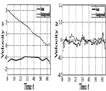
3.1 White Tower &Boat Synthetic Sequence
The synthetically generated sequence contains a moving object (boat) on a moving background (White Tower). The frame size is 296* 296 and the sequence’s length is frames T = 64. The background moves with
velocity pixel/frame and the boat
decelerates according to
pixels/frame.
For this experiment, White Gaussian Noise with SNR=32dB was added. We use the spectrogram because of its simplicity. The window used to obtain the Short-Time
Fourier Transform is a. In the TFR images, we search for two peaks along for each time instant. This is equivalent to applying the proposed Hough-transform methodology on TFR slices of length. Although, the spectrogram presents interference terms and bad localization, the estimated instantaneous velocities using FCP are very close to the real ones, as can be realized.
3.2Segmented Video with Velocity Estimation
White Tower & Boat-Frames 1, 32, 64 (three first figures) and the extracted layers, obtained applying (20) to the object’s images, taken using the proposed frequency-domain method, for the first 32 frames (last two figure)
OUTPUT VIDEO FRAME
Figure 2: White Tower & Boat-estimated instantaneous velocities.
ESTIMATION OF VELOCITY IN X AND Y PLANE
Figure 3: White Tower &Boat-motion segmentation results using graph-cuts for the frames 1, 10 and 20
IV.
CONCLUSION
127
Copyright © 2016. Vandana Publications. All Rights Reserved.
move with time-varying velocities. For this task, TFR was the appropriate, selected signal processing tool. We applied the Hough transform in overlapping time-slices of the TFR images to increase the robustness against noise and interference terms, present in the TFRs. Moreover, by exploiting the instantaneous frequencies estimates obtained for many spatial frequency pairs using FCP, we increased the robustness and accuracy of our method. Having estimated accurately the objects velocities, the proposed objects segmentation approaches produced correct and meaningful results. The experiments on various synthetic and natural sequences verified the effectiveness of the proposed method.
REFERENCES
[1] S.Barbarossa, Analysis of multicomponent LFM signals by a combined Wigner-Hough transform, IEEE Trans. Signal Process., 43(6): 1511–1515, 1995.
[2] W.-G. Chen, G. B. Giannakis, and N. Nandhakumar, Spatiotemporal approach for time-varying global image motion estimation, IEEE Trans. Image Process., 5(10): 1448–1461,1996.
[3] L. Cohen, Time-frequency distributions: A review, Proc. IEEE, 77(7): 941–981, 1989.
[4] I. Djurovic and S. Stankovic, Estimation of time-varying velocities of moving objects by time-frequency representations, IEEE Trans. Image Process., 12(5): 550– 562, 2003.
[5] C. E. Erdem, G. Z. Karabulut, E. Y. Yanmaz, and E. Anarim, Motion estimation in the frequency domain using fuzzy c-planes clustering, IEEE Trans. Image Process., 10(12):1873–1879, 2001.
[6] H. H. Nagel and E. Enklemann, An investigation of smoothness constraints for the estimation of displacement vector fields from image sequences,’ IEEE Trans. Pattern Anal. Mach. Intell., 8(9): 565–593, 1986.
[7] B. A. Watson and A. J. Ahumada, Model of human visual-motion sensing, 2(8): 322–342, 1985.
[8] J. Y. A. Wang and E. H. Adelson, Representing moving images with layers, IEEE Trans. Image Process., 3(9): 625–638, 1984.