A branch-and-bound procedure for the resource-constrained project scheduling problem with generalized precedence relations.

ECONOMISCHE WETENSCHAPPEN

ONDERZOEKSRAPPORT NR 9613

A Branch-and-Bound Procedure for the

Resource-Constrained Project Scheduling

Problem with Generalized Precedence Relations

by

Bert DE REYCK

Willy HERROELEN

Katholieke Universiteit Leuven

A Branch-and-Bound Procedure for the

Resource-Constrained Project Scheduling

Problem with Generalized Precedence Relations

0/1996/2376/13

by

Bert DE REYCK

Willy HERROELEN

RESOURCE-CONSTRAINED PROJECT SCHEDULING

PROBLEM WITH GENERALIZED PRECEDENCE RELATIONS

Bert DE REYCK

Willy HERROELEN

Operations Management Group Department of Applied Economics

Katholieke Universiteit Leuven Hogenheuvel College

Naamsestraat 69, B-3000 Leuven, Belgium Phone: 32-16-32 69 66 or 32-16-32696970

Fax: 32-16-32 67 32

E-mail: [email protected]@econ.kuleuven.ac.be WWW -page: http://econ.kuleuven.ac.be/tew/academic/om/people/bert

A

BRANCH-AND-BOUND PROCEDURE FOR THE

RESOURCE-CONSTRAINED PROJECT SCHEDULING PROBLEM WITH

GENERALIZED PRECEDENCE RELATIONS

Bert De Reyck • Willy Herroelen

Departement Toegepaste Economische Wetenschappen, Katholieke Universiteit Leuven

ABSTRACT

We present an optimal procedure for the resource-constrained project scheduling problem (RCPSP) with generalized precedence relations (further denoted as RCPSP-GPR) with the objective of minimizing the project makespan. The RCPSP-GPR extends the RCPSP to arbitrary minimal and maximal time lags between the starting and completion times of activities. The procedure is a depth-first branch-and-bound algorithm in which the nodes in the search tree represent the original project network extended with extra precedence relations which resolve a resource conflict present in the parent node. Resource conflicts are resolved using the concept of minimal delaying alternatives, i.e. minimal sets of activities which, when delayed, release enough resources to resolve the conflict. Precedence- and resource-based lower bounds as well as dominance rules are used to fathom large portions of the search tree. The procedure can be extended to other regular measures of performance by some minor modifications. Even non-regular measures of performance, such as the maximization of the net present value of the project or resource levelling objectives, can be handled. The procedure has been programmed in Microsoft® Visual C++ for use on a personal computer. Extensive computational experience is obtained.

KEYWORDS

1. Introduction

CPM (Critical Path Method; Kelley and Walker, 1959) and PERT (Program Evaluation and Review Technique; Malcolm et al., 1959) are basically devoted to project scheduling under the assumption that required resources are available in sufficient amounts, and that the

technological precedence relations between any pair of activities i and j imply strict precedence,

meaning that activity i must be completed before activity j can be initiated. For many years, the

assumption of sufficiently available resources has been relaxed and many research efforts have been directed towards project scheduling with explicit consideration of resource requirements and constraints. Davis (1973) categorized these models into three classes: time/cost trade-off problems, resource-constrained project scheduling problems and resource levelling problems.

More recent research has been directed at relaxing the strict precedence assumption of CPMlPERT. The resulting types of precedence relations are often referred to as MPM (Metra Potential Method) precedence constraints (Kerbosh and Schell, 1975; Zhan, 1994), precedence diagramming relations (Moder et al., 1983), time windows (Bartusch et al., 1988), minimal and maximal time lags (Brinkmann and Neumann, 1994; Neumann and Schwindt, 1995; Schwindt, 1995; Neumann and Zhan, 1996), and generalized precedence constraints (Wikum et al., 1994). In accordance with Elmaghraby and Kamburowski (1992), we denote them as generalized precedence

relations (GPRs). We distinguish between four types of GPRs: start-start (SS), start-finish (SF), finish-start (FS) and finish-finish (FF).

GPRs can specify a minimal or maximal time lag between any pair of activities. A minimal time lag specifies that an activity can only start (finish) when the predecessor activity has already started (finished) for a certain time period. A maximal time lag specifies that an activity should be started (finished) at the latest a certain number of time periods beyond the start (finish) of another activity. Many specific situations can be readily modelled using GPRs, such as (Bartusch et al., 1988; De Reyck, 1995b; Neumann and Schwindt, 1995):

• activity ready times (release dates) and deadlines • activities that have to start (terminate) simultaneously

• activities that have to terminate (can only start) x time units before the project completion • non-delay execution of (precedence related or unrelated) activities

• total overlapping / strong partial overlapping / weak partial overlapping of activities • fixed activity starting times

• time-varying resource-requirements and / or resource availabilities • time-windows for resources

• inventory (work in process) restrictions

• setup times, overlapping production activities (process batches, transfer batches) • assembly line zoning constraints

The first treatment of GPRs is due to Kerbosch and Schell (1975), based on the pioneering work of Roy (1962). Other studies include Crandall (1973), Elmaghraby (1977), Wiest (1981), Moder et al. (1983), Bartusch et al. (1988), Elmaghraby and Kamburowski (1992), Brinkmann and Neumann (1994), Zhan (1994), De Reyck (1995a, 1995b), Neumann and Schwindt (1995) and Schwindt (1995) and Neumann and Zhan (1996). Demeulemeester and Herroelen (1996a) have extended their branch-and-bound procedure for the RCPSP to the case of minimal time lags, activity release dates and deadlines and variable resource availabilities. To the best of our knowledge, the only optimal solution procedure reported in the literature for the RCPSP-GPR is the branch-and-bound procedure of Bartusch et al. (1988). Heuristic solution procedures are provided by Brinkmann and Neumann (1994), Zhan (1994) and Neumann and Zhan (1996). In this paper we present a new branch-and-bound procedure for the RCPSP-GPR supported by extensive computational tests.

The remainder of this paper is organized as follows. Section 2 elaborates on the concept of GPRs. Section 3 continues with the temporal analysis of activity networks with GPRs. In section 4 , which discusses the resource analysis of such networks, a branch-and-bound procedure for the RCPSP-GPR is presented. Computational results are given in section 5. Section 6 is reserved for our overall conclusions and suggestions for future research.

2. Generalized precedence relations (GPRs)

The extension of the Critical Path Method (CPM) to networks with GPRs was originally

called the Metra-Potential Method (MPM; Kerbosh and Schell, 1975). A basic assumption of CPM is that the precedence relations between the activities are of the finish-start type (with a time lag of zero). They imply a strict precedence because the predecessor activity must be completed before the successor activity can be initiated. These CPM networks can be represented by an acyclic activity-on-arc network, as in the original work of Kelley and Walker (1959), or by an acyclic activity-on-node network, which has gained more popularity.

CPM can easily be extended to GPRs, but only in the case of minimal time lags between activities, or, more correctly, only in the special case in which there are no arcs with negative length in the constraint digraph (cf. infra) and, consequently, no cycles of precedence relations. The same applies to the resource-constrained project scheduling problem (RCPSP), which can easily be extended to cope with minimal time lags (Demeulemeester and Herroelen 1996a). Activity networks with GPRs, however, can deal with activities among which maximal, as well as minimal time lags exist. The precedence relations specifying a maximal time lag can be represented by a negative minimal time lag in the opposite direction. Consequently, networks that include activities among which minimal and maximal time lags exist can be represented as

cyclic networks. For instance, a maximal finish-start lag of 5 between activity i andj is equivalent

to a minimal start-finish lag of -5 between activity j and i, as is shown in Fig. 1.

~

~~--~

Figure 1. The equivalence of maximal and minimal time lags

Assume a project represented in activity-on-node (AoN) notation by a directed graph G

=

{V, E) in which V is the set of vertices or activities, and E is the set of edges or GPRs. The

non-preempt able activities are numbered from 1 to n, where the dummy activities 1 and n mark the

beginning and the end of the project. The duration of an activity is given by di(1 S; i S; n), its

starting time by si (1 S; i S; n) and its finishing time by

1i.<1

S; i S; n). There are m renewable

resource types, with rikx (1 S; i S; n, 1 S; k S; m, 1 S; x S; di ) the resource requirements of activity i with

respect to resource type k in the xth period it is in progress and akt (1 S; k S; m; 1 S; t S; T) the

availability of resource type k in time period ]t-1, t] (T is an upper bound on the project length). If

the resource requirements and availabilities are not time-dependent, they are represented by

rik (lS;iS;n, lS;kS;m) and ak(lS;kS;m) respectively. The minimal and maximal time lags

between two activities i andj have the form:

The different types of GPRs can be represented in a standardized form by reducing them

to just one type, e.g. the minimal start-start precedence relations, using the following transformation rules (Bartusch et aI., 1988):

Si + SS[J'in S; S j = } si + _{lij S; S j} with _{lij =} SS[j'in

Si + SS;'J'ax 2 S j = } _{S j} + _{l ji S; Si} with lji =-SS[rX

s· _I + Sp.min _!] < _- f. _J = } _si + _{lij S; S j} with loo =Sp.min -d.

!] !] ]

s· + Sp.max > f.

I I] - J = } s·+l .. <s· J JI - I with l .. JI = d . -J SF·f!1ax !]

fi + FS[J'in S; S j = } _{Si +lij S;Sj} with lij = d i + FS[j'in

{,. + _I FSID.ax _!] >s. _{- J} = } _Sj + _{lji S; Si} with I ji = -di -

FS[j'ax

f.

_I + Fp.min _!] < _- f· _J = } _si+1ijS;Sj with lij = d i - d j +

FFijin

{,. + _, Fp.max _!] > _- f. _J = } _{S j} + _{I ji S; si} with I .. = d . - d. - Fp.max

If there is more than one time lag lij between two activities i and}, only the maximal time

lag is retained. The interval [so + l .. , s. - l .. ] is called the time window of s. relative to s. (Bartusch

' U ' ' J J '

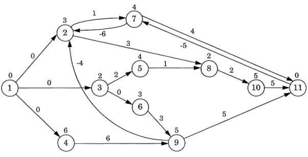
et aL, 1988). Applying these transformation rules to an activity network with GPRs results in a so-called constraint digraph, which is short for digraph of temporal constraints (Bartusch et aL,

1988). An example of such a constraint digraph is given in Fig. 2. The labels above the nodes

denote the activity durations d .. _, The labels associated with the arrows indicate the time lags

z...

_U

The constraint digraph contains less information than the original activity network. For instance, the effect of an increase or decrease in activity durations cannot be examined correctly in the constraint digraph. This, however, only poses a problem when the activity duration is subject to change as in time/cost trade-off problems or in multi-mode problems.

o

Figure 2. Constraint digraph of an activity network with GPRs

Because activity networks with GPRs contain cycles, additional concepts are needed (Bartusch et aL, 1988). A path <is' ik , il' ... , it> is called a cycle if s = t. With 'path' we mean a

directed path, and with 'cycle' we mean a directed cycle. The length of a path (cycle) is defined as

the sum of all the lags associated with the arcs belonging to that path (cycle). Activity durations do not have to be included in the calculation of a path length, since all time lags lij in a constraint digraph are of the SS-type. To ensure that the dummy start and finish activities correspond to the beginning and the completion of the project, we assume that there exists at least one path with

nonnegative length from node 1 to every other node and at least one path from every node i to

node n which is equal to or larger than di• If there are no such paths, we can insert arcs (l,i) or

(i,n) with weight zero or di respectively. In the example in Fig. 2, such arcs were added between

the set of all immediate predecessors of node i, Q(i)

=

{j

I

(i,j) E E} is the set of all its immediate successors. If there exists a path from i to j, then we call i a predecessor of j and j a successor of i.

p* (i) and Q* (i) denote the set of predecessors and successors of node i respectively. If the length

of the longest path from i to j is positive or all arcs of a longest path are associated with a lag of

zero, node i is called a real (immediate) predecessor of node j, and j is called a real (immediate)

successor of i. Otherwise it is a fictitious one.

3. Temporal analysis

The goal of project scheduling problems is to obtain a schedule B, which is a vector of starting times {sl' s2' ... , snl for all activities. Schedules are subject to temporal constraints and resource constraints. In this section, we focus on the temporal constraints. In section 4, additional resource constraints will be taken into account. A schedule is called time-feasible, if all the starting times satisfy all (generalized) precedence relations. In other words, a time-feasible

schedule with starting times {s l' s2' ... , snl satisfies the conditions that:

{

Si ;;::

°

s· I +l·· lJ -< s· J

[1]

[2]

where Eqs. 1 ensure that no activity starts before the current time (time zero), and Eqs. 2 denote the precedence constraints in standardized form. Notice that Eqs. 1 have to be included, not only

for the starting activities, but for every activity in the network, since the time lags lij can assume

negative values. The minimum starting times {Sl' S2' ••. , sJ satisfying both Eqs. 1 and 2 form the

early start schedule EBB = {es l ' es2, ... , esnl associated with the temporal constraints. For the

example, EBB = {O, 2, 0, 0, 2, 0, 7, 5, 6, 7, 12l, as represented by the Gantt-chart in Fig. 3. The

arrows indicate the time lags that are binding. The dotted line represents the end of the project (finishing time of the dummy end activity).

The calculation of an EBB can be related to the test for existence of a time-feasible

schedule. The earliest start of an activity i can be calculated by fmding the longest path from node

1 to node i. We also know that there exists a time-feasible schedule for G iff G has no cycle of

positive length (Bartusch et al., 1988). Cycles of positive length would unable us to calculate starting times for the activities which satisfy conditions [1] and [2]. Therefore if we calculate the

distance matrix D = [dijl, where dij denotes the maximal distance (path length) from node i to

node j, a positive path length from node i to itself indicates the existence of a cycle of positive

Activities 11 10 9 8 7 6 5 4 3 2 1 ~ , .. ',.

...

-.

-I 1

..

... -I 1 1 1 ·.···,··".·,1 1 1 I I I I I I I I 1 I I

i

I

I

I

1

I

I

I

I

I

I

I

I

1 2 3 4 5 6 7 8 9 10 11 12 Time

Figure 3. A Gantt-chart of the ESS

The calculation of the distance matrix D can be done by standard graph algorithms for

longest paths in networks, for instance by the Floyd-Warshall algorithm (for details, see Lawler,

1976). Ifwe start with the matrix D(l)

=

[di~l)] (i,j = 1,2, ... , n) with

ifi= j \:j (i, j) E E

otherwise

we can compute the matrix D

=

Din_{+1) according to the updating formula}

di~u)

=

max{d&U-l) ,di~u-l) + d t1)} (i, j, l = 1, 2, ... , n). If d ii = 0 for all i = 1, 2, ... , n (the numbers in

the diagonal of D), there exists a time-feasible schedule. The ESS is given by the numbers in the

upper row of D: ESS = _{{d ly d l,2' ... , dl,n}'}

The computation of D takes O(

I

V1

3) time (Bartusch et ai., 1988). The ESS can be

calculated more efficiently by using the Modified Label Correcting Algorithm (Ahuja et al., 1989),

which is of time complexity O(

I

V

I I

E

I)

and which also allows for the identification of positive

cycles and for the calculation of a late start schedule LSS = {lsI' lS2' ... , lSn}' The existence of

positive cycles can also be verified by employing the modified Bellman algorithm of time

complexity O(

I VI I

E

I),

and the identification of such cycles can be accomplished by the algorithm

4. Resource analysis

The resource-constrained project scheduling problem with generalized precedence relations (RCPSP-GPR) can be conceptually formulated as follows:

Minimize sn Subject to sj+lijS;Sj I,rik S; akt iES(t) sl == 0 No splitting allowed k == 1,2, ... ,m t == 1,2, ... , T i == 1, 2, ... , n

[3]

[4]

[5]

[6]

[7]

where S(t) is the set of activities in progress in time period ]t-1, t] and T is an upper bound on the

project duration, for instance T ==

I,

maX{di , ;max. {lij}} (for the example in Fig. 2, T == 34). Note

iEV JEQ(£)

that it is not always possible to derive a feasible solution. The upper bound T indicates the

maximal value for the project makespan if a feasible solution exists. The objective function given

in Eq. 3 minimizes the project duration, given by the starting time (or finishing time, since dn == 0)

of the dummy activity n. The precedence constraints are denoted in standardized form by Eqs. 4. Eqs. 5 represent the resource constraints. The resource requirements and availabilities are assumed to be constant over time, although this assumption can be easily relaxed using GPRs without having to change the solution procedures (Bartusch et al., 1988). Eq. 6 forces the dummy start activity to begin at time zero and Eqs. 7 ensure that the activity starting times assume nonnegative integer values. Once started, activities run to completion. However, this nonpreemption condition can easily be relaxed by splitting up the activities in unit-duration

subactivities (Demeulemeester and Herroelen, 1996b), connected with strict precedence relations (zero-lag finish-start precedence relations).

The RCPSP-GPR is known to be strongly NP-hard, and even the decision problem of testing whether a RCPSP-GPR instance has a feasible solution is NP-complete (Bartusch et aI.,

1988). Demeulemeester and Herroelen (1996a) developed a branch-and-bound procedure for the

generalized resource-constrained project scheduling problem (aRCPSP) which allows for minimal time lags only, with the additional assumption that a successor activity can never start before its predecessor (i.e. no negative lags in the constraint digraph). To the best of our knowledge, the only optimal solution procedure presented in the literature for the RCPSP-GPR is the bound algorithm of Bartusch et ai. (1988). In this section, we discuss a new branch-and-bound procedure for the RCPSP-GPR based on the concepts of minimal delaying alternatives as developed by Demeulemeester and Herroelen (1992) for the RCPSP and adapted by Icmeli and

Erengiic; (1996) for the RCPSP with discounted cash flows. The procedure uses several lower bounds, including a generalized version of a lower bound for the RCPSP proposed by Mi..Tlgozzi et al. (1994) and several powerful dominance rules.

4.1. The search tree

The nodes in the search tree represent the initial project network, described by a distance

matrix

D

=

[dij] ,

extended with extra (zero-lag finish-start) precedence relations to resolve a

resource conflict present in the parent node, which results in an extended distance matrix. Nodes which represent time-feasible (no violated maximal time lags) but resource-infeasible project networks and which are not fathomed by any node fathoming rules described below lead to a new branching. Therefore each (undominated) node represents a time-feasible, but not necessarily resource-feasible project network. A similar branching scheme is used by Bartusch et al. (1988). However, these authors use the concept of a reduced forbidden set (a minimal set of activities which cannot be scheduled together within the resource constraints) to resolve the resource conflicts. Resource conflicts are then resolved by successively adding precedence relations such that each forbidden set is no longer scheduled in parallel. Each possible combination of added precedence relations leads to a new node. A similar branching scheme as the one of Bartusch et al. (1988) was used by Bell and Park (1990) for the RCPSP. Bell and Park (1990) use the concept of a minimal resource violating set, which is equivalent to a reduced forbidden set.

In our procedure, resource conflicts are resolved using the concept of minimal delaying

alternatives (Demeulemeester and Herroelen, 1992), i.e. minimal sets of activities which, when delayed, release enough resources to resolve the resource conflict (and which do not contain any other delaying alternative as a subset). Each of these minimal delaying alternatives is then

delayed (enforced by extra strict precedence relations i -< j , implying Si + di ::; S j ) by each of the

activities also belonging to the conflict set S(t*), the set of activities in progress in period ]t*-1, t*] (the period of the first resource conflict), but not belonging to the delaying alternative.

A similar delaying strategy was used by Demeulemeester and Herroelen (1992) for the RCPSP. As the RCPSP can be solved using semi-active timetabling to construct the partial schedules, activities belonging to the minimal delaying alternative can be delayed by the activity in S(t*) which terminates at the earliest time instant after the current decision point. In the RCPSP-GPR, this delaying strategy cannot be used because of the presence of maximal time lags, which make semi-active timetabling inappropriate. The same problem occurs in the RCPSP with discounted cash flows (RCPSP-DC). In the RCPSP-DC, semi-active timetabling is also inappropriate and a modified delaying scheme has to be used. Icmeli and Erengiic; (1996) have

modified the delaying scheme of Demeulemeester and Herroelen (1992) for the RCPSP-DC. A similar scheme can be used for the RCPSP-GPR.

There are several possible delaying modes for delaying a delaying alternative. In the procedure of Demeulemeester and Herroelen (1992), no distinction was needed between minimal delaying alternatives and minimal delaying modes because there was a one-to-one correspondence between the two. In the RCPSP-GPR, one delaying alternative can give rise to several delaying

modes, possibly one for each activity in S(t*) which is not an element of the delaying alternative.

Assume, for example, that in a certain period ]t*-l, t*], 4 activities are in progress and

cause a resource conflict: S(t*)

=

{1, 2, 3, 4}. Suppose that the minimal delaying alternatives are

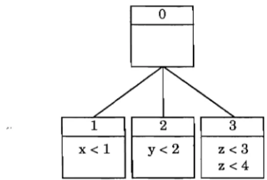
{I}, {2} and {3, 4}, i.e. delaying activity 1, activity 2 or activities 3 and 4 simultaneously releases enough resources to resolve the resource conflict. For the RCPSP, using the procedure of Demeulemeester and Herroelen (1992), we would create 3 new nodes (three minimal delaying

modes). In the first node, activity 1 is delayed by the earliest finishing activity (x) among

activities 2, 3 or 4 (x -; 1). In the second node, activity 2 is delayed by the earliest finishing

activity (y) among activities 1, 3 or 4 (y -; 2). Finally, activities 3 and 4 are delayed by activity 1

or 2 (z), depending on which activity finishes the earliest (z -; 3 and z -; 4). This results in 3 new

nodes, as illustrated in Fig. 4.

0

/

I~

1 2 3

x<l y<2 z<3 z<4

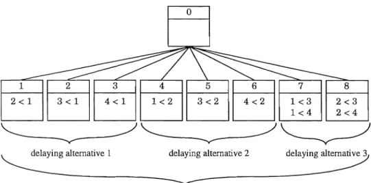
Figure 4. Delaying strategy for the RCPSP of Demeulemeester and Herroelen (1992) For the RCPSP-GPR, as for the RCPSP-DC (Icmeli and Erengii<;, 1996), the delay of

activity 1 is established by adding a precedence relation between activity 2, 3 or 4 and activity 1.

We therefore create three new nodes (instead of one), one with the precedence relation 2 -; 1, one

with the precedence relation 3 -; 1 and one with the precedence relation 4 -< 1. Delaying activity 2

is accomplished by creating 3 new nodes with the extra precedence relations 1-< 2, 3 -; 2 and 4 -< 2. Delaying activities 3 and 4 is accomplished by creating two new nodes with the extra precedence relations 1-< 3 and 1-; 4, or 2 -; 3 and 2 -< 4. In total, 8 new nodes (minimal delaying modes) are created, as illustrated in Fig. 5.

o

1 8

2<1 3<1 4<1 1<2 3<2 4<2 1<3 2<3 1<4 2<4

delaying alternative 1 delaying alternative 2 delaying alternative 3

8 delaying modes

Figure 5. Delaying strategy for the RCPSP-GPR

In general, the delaying set D, i.e. the set of all minimal delaying alternatives, is equal to

D

=

{Dd Dd c S(t*) and \;j resource type k: I.rik - I.rik :5; ak and \;j Dd, ED: Dd, (J:. Dd}. The iES(t*) iEDd

set of minimal delaying modes equals:

M

=

{Mml Mm

=

{k

-< Dd}, k E S(t*) \ Dd , Dd ED}. Activity

k is called the delaying activity: k -< Dd implies that k -< l for all l E Dd .

Each minimal delaying mode is then examined for time-feasibility and, if time-feasible, evaluated by computing the critical path based lower bound Lbo. Each time-feasible minimal delaying mode with a lower bound Lbo:::; T is then considered for further branching, and branching occurs from the node with the smallest lower bound Lbo. If the node represents a

project network in which a resource conflict occurs, a new branching occurs. If it represents a

feasible schedule, the lower bound T is updated and the procedure backtracks to the previous

level in the search tree. Therefore, we have a depth-first search procedure, in which branching occurs until at a certain level in the tree, there are no delaying modes left to branch from. Then, the procedure backtracks to the previous level in the search tree and reconsiders the other delaying modes (not yet branched from) at that level. The procedure stops when it backtracks to levelO.

THEOREM 1. The delaying strategy which consists of delaying all minimal delaying alternatives

Dd by each activity k E S(t*) \ Dd will lead to the optimal solution of the RCPSP-GPR in a finite number of steps.

4.2. Node fathoming rules

Nodes are fathomed when they represent a time-infeasible project network or when lb_o

exceeds T. Nodes which are not fathomed and still represent an infeasible project network are

considered for further branching. Four other node fathoming rules are added, three dominance rules and a lower bound rule. We also add a procedure which reduces the solution space.

4.2.1. Redundant delaying alternatives

Because activity overlaps are allowed (dij < d), it is possible that in period ]t*-l, t*] (the

period ofthe first resource conflict), the set of activities in progress (the conflict set S(t*» contains

an activity i together with a real successor j of activity i (dij ~ 0). Then, delaying activity i will

inevitably also delay activity j. Therefore, we can extend each minimal delaying alternative D d

with the real successors j (j!t: Dd ) of an activity i E Dd • As a result of this operation, minimal

delaying alternatives may become non-minimal, which can be eliminated from further consideration.

THEOREM 2. If there exists a minimal delaying alternative D d with activity i E D d but its real

successor j!t: Dd (dij ~ 0), we can extend Dd with activity j. Any minimal delaying alternative becoming non-minimal as a result of this operation may be eliminated from further consideration. PROOF. Obvious.

4.2.2. Redundant delaying modes

Again, because of the possibility of activity overlaps, it is possible that a certain minimal

delaying alternative Dd is giving rise to two delaying modes M m _, and M m ₂ ,in which the delaying

activities i (i -< D d ) and j (j -< D d ) are precedence related. If dij + d j ~ di , that is, in any feasible

solution, activity j will terminate after activity i, we can eliminate delaying mode M m from

2

further consideration because it will never lead to a superior solution than delaying mode Mm.

_,

THEOREM 3. When a minimal delaying alternative D d gives rise to two delaying modes M m, and

M m with delaying activities i and j respectively, delaying mode M m is dominated by delaying

2 2

mode M m, iff dij + d j ~ di ·

4.2.3. A time- and resource-based lower bound

Recently, Mingozzi et al. (1994) have developed five new lower bounds, IbI , lb2 , lbp ' lbx

and lb3 , derived from different relaxations of a new mathematical formulation for the RCPSP.

Some of these new lower bounds (namely lbI , lb2 , lbx and lb3 ) dominate the critical path based

lower bound (lb o) and they all prove to be tighter than the critical sequence lower bound (lb) of Stinson et al. (1978) on the 110 RCPSP instances assembled by Patterson (1984) and the 480 randomly generated RCPSP instances of Kolisch et al. (1992). Mingozzi et al. (1994) have also developed a new branch-and-bound procedure for the RCPSP based on this new mathematical

formulation, which incorporates the most promising new lower bound lb3 .

Mingozzi et al. (1994) compute lb3 using a heuristic for the weighted node packing

problem. Demeulemeester and Herroelen (1995) have incorporated another version of Ib3 (lb;) in

their procedure for the RCPSP: For each activity i E V, its possible companions, i.e. the activities

with which it can be scheduled in parallel, respecting both the precedence and resource

constraints, are determined. All (unscheduled) activities i are then entered in a list L in

non-decreasing order of the number of companions (non-increasing duration as tie-breaker). The following procedure then yields a lower bound, lb; (for the partial schedule under consideration):

lb; = 0 (or the earliest completion time of the activities in progress if a partial schedule is

already determined)

while L not empty do

take the first activity (activity i) in L

lb; = lb; + di

remove activity i and its companions from L

enddo

Computational results obtained by Demeulemeester and Herroelen (1995) indicate that

lb; indeed outperforms lbo and that incorporating lb; in their branch-and-bound procedure

reduces the computational effort to solve the 110 problems of Patterson (1984) and the 480

problems of Kolisch et al. (1992). Note that, contrary to lb3 as calculated by Mingozzi et al. (1994),

the procedure above may yield an lb; which is smaller than lbo, but this constitutes no real disadvantage since lbo is calculated as well and the final value for the lower bound equals

The procedure of Demeulemeester and Herroelen (1995) for computing lb~ can be extended to the RCPSP-GPR, by changing the calculation of the companions of the activities. In the RCPSP-GPR, two activities i and j between which a precedence relation exists, are companions if the resource requirements of both activities do not exceed the resource availability for any resource type, and if both dij < di and dji < dj .

In our implementation of Ib3 , we have also adapted the (weighted node packing) heuristic.

Instead of removing an activity j from the list L when a companion i is taken from the list, we

only remove part of activity j from the list. The logic behind this reasoning relies on both a

duration and time lag argument. The duration argument goes as follows: When an activity i is

scheduled, a companion j can be scheduled in parallel with i. However, if di < dj , only a part of

activity j can be scheduled in parallel with i. Therefore, a part of activity j (with remaining

duration d'j

=

d j - d_{i )} can be left in L. Initially, all d'j are equal to dj .

It is clear that Ib3 , even using the duration argument as described above, will not perform

as well as lb; did for the RCPSP without GPRs. The reason for this is that activities will have

many more companions in the RCPSP-GPR than in the RCPSP. Even when activities i andj can

overlap for only one time unit (because of a minimal start-start time lag equal to di - 1), they will

be considered as companions. Therefore, when using Ib3 for the RCPSP-GPR in an effective way,

we will have to look at the time lags between the activities, leading to our time lag argument: We

adjust the part of activity j which has to be removed when a companion i is taken from the list, by

incorporating the precedence relations between i and j. Suppose, for instance, that two

companion-activities, i and j, are in L (di

=

3, dj

=

5 en Ii)

=

2). Using the heuristic of

Demeulemeester and Herroelen (1995), we would remove activity j from the list when activity i is

taken from the list, which leads to an increase in Ib~ by di • Using our duration argument made

above, we would leave activity j in the list, but only with a duration d'j equal to dj - di = 2. If no

other companion of j is taken from the list, Ib3 could be as much as two units higher than in the

case where activity j would be completely removed from L. Taking into account the start-start

precedence relation Iij = 2 between i and j, we see that activity i and j can only overlap for one

time unit. Therefore, using our time lag argument, only one time unit has to be subtracted from

dj , possibly leading to a further increase in Ib3 •

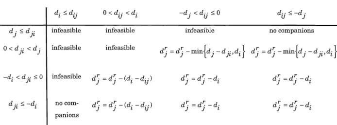
However, several different types of activity overlaps may occur. Therefore, we have to look

deciding how much to remove from activity j. Table I shows the appropriate action (namely how

much to remove from activity j) for each combination. Note that when we want to remove x units

from activity j whereas only y (y<x) units are left, activity j is to be removed completely from L.

Table 1. The calculation of d'j

d· <d·· _{~ - U} O<d·· <d· _{U ~} -d· _J < d·· < _u-0 d·· <-d· _~J

- J

d· < d·· infeasible infeasible infeasible no companions

J - J~

O<d··<d· infeasible infeasible _{dT". =dT". -min{d. -d·· d.} dT". =dT". -min{d. -d·· d.}}

J~ J _{J J J J~' ~ J J J F' ~} -d· ~ < d·· F -< 0 infeasible dT". =dT". -(d· -d··) dT". = dT". - d· dT". = dT". -d· J J ~ U J J ~ J J L d·· < -d· no com- _{dT". =dT". -(d· -d··) dT".=dT".-d· dT". =dr. -d·} JL - ~ J J ~ U J J L J J L panions

Because in an optimal solution procedure for the RCPSP-GPR, time-infeasibilities will be

detected before lb3 is calculated, the calculation of lb3 for the RCPSP-GPR (lbl) can now be

summarized as follows:

lbl

=

0

while L not empty do

enddo

take the first activity (activity i) in L and remove it from L

lbl

=

lbl + d[

for every companionj of i do

if l·· > 0 then dr

₌

_{dr - (d· - d··)}

U J J ! U

else if l·· > 0 then d~

=

dr _{-min{d. -d·· d.}}

J! J J J J ! ' !

else dr

=

d~ _{- d·}

J J !

endif

if d'j :::; 0, remove activity j from L

enddo

THEOREM 4. lbl is a valid lower bound for the RCPSP-GPR.

lbf is used to fathom nodes for which lbf:2: T. However, whereas lb o is calculated

immediately upon the creation of a node, the calculation of lbf is deferred until a decision has been made to actually branch from that node. The rationale behind this is that (a) lbf is much more difficult to compute than lbo, and that (b) calculating lbf implies calculating the entire

distance matrix (time complexity

O[n

2 ] using the algorithm described in section 4.3). Supported

by extensive computational tests, we defer the calculation of lbf and the distance matrix until the node is actually selected for branching. As a result, only lbo is used as a branching criterion. Time-infeasibilities (which lead to node fathoming) or feasible solutions (which lead to an upper bound update) are also detected only when that node is selected to branch from.

4.2.4. A subset dominance rule

The branch-and-bound procedure starts with the early start schedule for the project network in the root node of the search tree, and successively adds precedence constraints in order to eliminate resource conflicts. Each node represents the initial project network extended with a set of (strict) precedence constraints. Therefore, it is possible that a certain node represents a project network which has been examined earlier at another node in the search tree, in which case the corresponding distance matrices will be identical. Therefore, it suffices to compare these distance matrices. However, saving and comparing distance matrices would lead to an enormous increase in memory requirements and computational effort. Another way of checking whether two nodes represent the same project network, is to check the added precedence constraints. Identical sets of precedence constraints lead to identical project networks. Examining the sets of precedence constraints also allows us to check whether a set of precedence constraints in a node contains as a subset another set of precedence constraints obtained in another node, in which case the former node can be eliminated from further consideration, since it can never lead to a superior solution.

THEOREM 5. If the set of added precedence constraints which leads to the project network (in the

form of an extended distance matrix) in node x contains as a subset another set of precedence constraints leading to the. project network (extended distance matrix) in a previously examined node y in another branch of the search tree, node x can be fathomed.

PROOF. See appendix.

Notice, however, that the set of added precedence constraints in a certain node always contains as a subset the set of precedence constraints in its parent node (or grandparent node, ... ). Obviously, this rule only applies when a set of precedence constraints is compared to another set of precedence constraints obtained along another path of the search tree. This can easily be enforced by only saving information for node dominance testing during backtracking.

The question remains which nodes exactly have to be saved in order to be able to test this

dominance rule. When a node x is dominated by a node y, it will also be dominated by a node z

which is the parent node of node y unless it is also a parent node of node x. Therefore, to check

whether node x is dominated, we save the set of added precedence constraints of the nodes which

are no parent node of x, but for which the parent node is a parent node of x. Suppose that for the example search tree in Fig. 6, all nodes on a certain level are sorted from left to right in

nondecreasing order of Lbo (which is the order in which they will be selected to branch from). In

order to examine whether node x is dominated by another node examined earlier, we only have to

examine all nodes displayed in bold. All other nodes are either a parent node of node x, or contain

no useful information since a parent node can equally well dominate node x. When we reach node

x, only the information concerning the four bold nodes has to be saved in order to be able to test

node dominance.

Figure 6. A conceptual search tree

Consequently, all the information which is needed to test this dominance rule can be

saved very efficiently as follows: When the procedure backtracks into a node at level p of the

search tree, save the set of added precedence relations of that node (with respect to the original problem, not with respect to the parent node) on a stack. Before doing that, however, delete from the stack all the information which has been saved on level p+l. This guarantees that all the required information for dominance testing is saved on the stack, and removed when it is no longer required. The set of added precedence constraints from nodes that are feasible (yielding an upper bound), time-infeasible (because maximal time lags are violated) or fathomed need not be saved on the stack since all other nodes which contain that set as a subset will also be feasible, time-infeasible or fathomed.

4.2.5. Reducing the solution space using preprocessing

Before initiating the branch-and-bound procedure, the solution space can be reduced by

simultaneously examining the GPRs and the resource requirements. If on the one hand, two

activities i andj can never be companions due to the resource constraints, but on the other hand,

the (generalized) precedence relations allow for an overlap, then the precedence relations can sometimes be tightened in order to avoid the overlap. For instance, suppose that in the problem example of Fig. 2, activities 2 and 3 cannot be companions due to their resource requirements.

However, the maximal distances between activities 2 and 3 are d2,3 = - 0 0 and d_3,2 = -1 ,

indicating that an overlap is allowed. The only restriction is a maximal time lag between activity 2 and 3 of 1 time unit, implying that activity 2 can only start 1 time unit before activity 3. However, because activities 2 and 3 are no companions, they can never be scheduled in parallel (notice that activity 2 cannot start 1 time unit before activity 3 because then an overlap would

occur), such that the time lag between activities 3 and 2 can be increased to l3,2

=

d3

=

2.

THEOREM 6. If ::3 i, j E V and resource type k for which rik + rjk > ak and -d j < dij < d i , we can set lij = _{d i without changing ihe optimal solution of the RCPSP-GPR.}

PROOF. See appendix.

This rather straightforward rule is often very effective in reducing the solution space. Moreover, because it can be executed as a preprocessing rule, it is very efficient.

4.3. The branch-and-hound algorithm

The detailed algorithmic steps of the proposed branch-and-bound algorithm are described

below. The maximal distance between two activities

i

andj is given by

d[p][i](j],

wherep denotes

the level in the search tree. For each such level, a distance matrix

d[p]

will have to be stored. For

ease of reference, a numerical example is given in Appendix 1.

STEP 1: INITIALISATION

Let T = 9999 be an upper bound on the project duration.

Set the level of the branch-and-bound tree p

=

o.

Compute the constraint digraph cd (using the transformation rules discussed in section 2).

Compute

d[

0] , the distance matrix at level 0 using the Floyd-W arshall algorithm

(o[

n 3 ] ).

Ifthe project is not time-feasible (i.e. ::3 iE V:

d[O][i][i]

> 0), STOP.

Preprocessing: reduce the solution space by adjusting

d[O]:

V(i,

j)

I

i, j E V and ::3 resource type k : rik + rjk > ak and

case 1:

-dj

<

d[O][i][j]

<

di ,

set

lij

=

di

case 2:

_-di

<

d[O](j][i]

<

dj ,

set

lji

=

dj

Recompute

d[

0] using the Floyd-Warshall algorithm (

o[

n 3 ] ).

Compute the critical path based lower bound

Lbo

=

d[O][l][n]

and go to STEP 3.

STEP 2: TEMPORAL ANALYSIS

Compute

d[p],

the extended distance matrix at level

p

as follows:

Vi,j

E V:

d[p][i](j]

=

d[p -l][i](j]. Vi,j

E V,

l

E Dd:

d[p][i][j]

=

max{d[p][i][j], d[p-1][i][k]+d

k

+d[p -l][l)[j]}, k

being the delaying activity

(O[n

2 ]).

If T < 9999, compute lbf (using the algorithm described in section 4.2.).

If lbf ~ T, erase the delaying mode and go to STEP 6.

STEP 3: RESOURCE ANALYSIS

Determine the first period in which a resource conflict occurs, i.e. the first period ]t*-l, t*] for

which I,rik > ak for some resource type k. S(t*), the set of activities in progress in period

iES(t*)

]t*-l, t*], is called the conflict set.

If there is no conflict, let

T

=

min

{T,

d[p ][

1][

n ]},

erase the delaying mode and go to STEP 6.

STEP 4: DETERMINE MINIMAL DELAYING ALTERNATIVES AND MINIMAL DELAYING MODES

Increase the branch level of the search tree: p = p + 1.

Determine the minimal delaying set, i.e. the set of minimal delaying alternatives:

D

=

{Dd Dd c S(t*) and'll resource type k:

2>ik - I,rik

S;

ak

and'll Dd, ED: Dd, CZ Dd}

iES(t*) iED"

Extend all minimal delaying alternatives using Theorem 2 and eliminate all non-minimal delaying alternatives. Determine the set of minimal delaying modes:

M={Mml Mm ={k-<Dd},kES(t*)\Dd,Dd ED}. Eliminate all delaying modes satisfying Theorem 3.

Arbitrarily select a delaying mode Mm with corresponding delaying alternative D d'

STEP 5: EVALUATE DELAYING MODES

For all delaying modes M m {

Ifthe precedence constraints cannot be added, i.e. 3l E Dd: k -< l is infeasible, i.e.

dk > -d[p][l][k] (k being the delaying activity), continue with next delaying mode Mm'

Compute Lbo as follows: Set Lbo

=

d[p

-l][l][n].

'Ill E Dd and delaying activity k:

Lbo = max{lbo, d[p

-l][l][k]

+ dk + d[p -l][l][ n]

I

j E Dd}' If Lbo 2: T , continue with next delaying mode Mm'

If the set of added precedence constraints of a previously examined node saved earlier is a subset of the set of added precedence constraints of the current node, continue with next

delaying mode Mm'

Calculate lb = Lbo.

Temporarily store the delaying mode and its lower bound lb.

STEP 6: BRANCHING

If no delaying modes are left to branch from at levelp, go to STEP 7.

Select the delaying mode Mm with the smallest lower bound lb = Lbo (arbitrary tie-break).

If lb 2: T , erase all remaining delaying modes at level p and go to STEP 7.

Go to STEP 2.

STEP 7: BACKTRACKING

Decrease the branch level of the search tree:p = p -1.

(if T = 9999, then there exists no feasible solution).

Delete from the stack the information which has been previously saved on levelp+1 for dominance testing.

Save the necessary information for node dominance testing on the stack, i.e. the list of added precedence constraints of the node reached upon backtracking.

Erase the distance matrix and the lower bound of this node and go to STEP 6.

4.4. A numerical example

Consider the example given in Fig. 2. Suppose there are two renewable resource types with a constant availability of 10 units each, and resource requirements for each of the activities

equal to {O, 6, 5, 5, 6, 5, 3, 3, 2, 5,

o}

and

{o,

1, 3, 2, 7, 6, 3, 1, 1, 2, O} respectively. We will compute the

optimal solution by going through the steps ofthe algorithm.

STEP 1: T

=

9999 andp = O. Compute

d[O].

Lbo

=

d[O][l][ll]

=

12. The project is time-feasible.

Reduce solution space, i.e. set: l3,2 =

d

3 = 2 (-~(= -3) <

d[0][3][2]

(= -1) <

da(=

2) ), l4,2 =

d

4 = 6

(-d

2

(=

-3) <

d[O][

4][2] (= 2) <

d

4 (= 6) ),

l6,2 =

d

6 = 3 (-~(= -3) <

d[0][6][2]

(= -1) <

d

6(= 3», and l5,10 =

d

5 = 4

(-d

lO

(=

-5) <

d[O][5][10]

(= 3) <

d

5

(=

4) ).

Recompute

d[O],

Lbo =

d[O][l][ll]

= 16.

STEP 3: There is a resource conflict in period ]0,1]; 8(1) = {3,4,6}. Store the distance matrix.

STEP 4: p = 1.

D

= {{3}, {4},{6}}. Because

d[O][3][6];:::

0, Theorem 2 can be applied: extend

delaying alternative {3} with activity 6: D

=

{{3,6},{4},{6}}. Eliminate non-minimal delaying

alternative {3,6}: D = {{4},{6}}; M

=

{{3 -< 4},{6 -< 4},{3 -< 6},{4 -< 6}}. Because

d[0][3][6]

+

d

6

(=

0 + 3) >

da(=

2), we can eliminate mode {6 -< 4} since it is dominated by

delaying mode {3 -< 4}:M = {{3 -< 4},{3 -< 6},{4 -< 6}}.

STEP 5: Mode {3 -< 4}: The precedence constraint 3 -< 4 can be added. Initialize

Lbo

=

d[O][I][ll]

= 16. Lbo

=

max{lbo,

d[0][1][3]

+

d

3 +

d[0][4][1l]}=

max{16, 0 + 2 + 16}= 18 .

Lbo < T. No dominance information has been saved yet. Store the delaying mode and its lower

bound lb = Lbo = 18 . Mode {3 -< 6}: The precedence constraint 3 -< 6 can be added. Initialize

Lbo =

d[O][I][ll]

= 16. Lbo

=

max{lbo,

d[0][1][3]

+

d

3 +

d[0][6][1l]}=

max{16, 0 + 2 + 13}= 16.

Lbo < T. No dominance information has been saved yet. Store the delaying mode and its lower

bound lb

=

Lbo = 16 . Mode {4 -< 6}: The precedence constraint 4 -< 6 can be added. Initialize

Lbo =

d[O][l][ll]

= 16. Lbo = max{lbo,

d[O][I][4]

+

d

4 +

d[O][6][1l]}

= max{16,O+6+13}=19. Lbo < T. No dominance information has been saved yet. Store the delaying mode and its lower

bound lb = Lbo = 19 .

STEP 6: Select the delaying mode with the smallest lb, i.e. {3 -< 6}. lb < T.

STEP 2: Compute

d[l]. T

is still equal to 9999.

STEP4:p

=

2. D

=

{{5},{4,6}}. M

=

{{4 -< 5},{6 -< 5},{5 -< 4, 5 -< 6}}.

STEP 5: Mode {4 -< 5}: The precedence constraint 4 -< 5 can be added. Initialize

Lbo

=

d[l][l][l1]

=

16. Lbo = max{lbo,

d[l][l][

4] +

d

4 +

d[1][5][l1]}

= max{16, 0 + 6 + 9}= 16.

Note that

d[1][5][11]

= 9 instead of 8 because ofthe preprocessing performed in STEP l.

Lbo < T. No dominance information has been saved yet. Store the delaying mode and its lower

bound lb = Lbo = 16 . Mode {6 -< 5}: The precedence constraint 6 -< 5 can be added. Initialize

Lbo =

d[l][l][l1]

= 16. Lbo = max{lbo

,d[1][1][6]+d

6 +

d[1][5][l1]}

= max{16,2+3+9}=16.

Lbo < T. No dominance information has been saved yet. Store the delaying mode and its lower

bound lb = Lbo = 16 . Mode {5 -< 4, 5 -< 6}: The precedence constraints can be added. Initialize

Lbo =

d[l][l][l1]

= 16. Lbo = max{lbo,

d[1][1][5]

+

d

5 +

d[l][

4][11]} = max{16, 2 + 4 + 16}= 22. Lbo = max{lbo,

d[1][1][5]

+

d

5 +

d[1][6][11]}=

max{22, 2 + 4 + 13}= 22 .lbo <

T.

No dominance

information has been saved yet. Store the delaying mode and its lower bound lb = Lbo = 22.

STEP 6: Select the delaying mode with the smallest lb, i.e. {4 -< 5} (arbitrary tie-break with

{6

-<

5} ).

lb < T.

STEP 2: Compute

d[2].

T is still equal to 9999.

STEP 3: There is a resource conflict in period ]6,7]: 8(7) = {2,5,9}. Store the distance matrix. STEP 4:p = 3. D = {{2},{5}}. M = {{5 -< 2},{9 -< 2},{2 -< 5},{9 -< 5}}.

STEP 5: Mode {5 -< 2}: The precedence constraint 5 -< 2 can be added. Initialize

Lbo =

d[2][1][11]

= 16. Lbo = max{lbo,

d[2][1][5]

+

d

5 +

d[2][2][11]

}= max{16, 6 + 4 + 10}= 20. Lbo < T. No dominance information has been saved yet. Store the delaying mode and its lower

bound lb = Lbo = 20 . Mode {9 -< 2}: The precedence constraint 9 -< 2 can be added. Initialize

Lbo =

d[2][1][11]

= 16. Lbo = max{lbo,

d[2][1][9]

+

d

g +

d[2][2][11]}=

max{16, 6 + 5 + 10}= 2l. Lbo < T. No dominance information has been saved yet. Store the delaying mode and its lower

bound lb = Lbo = 21. Mode {2 -< 5}: The precedence constraint 2 -< 5 cannot be added since

d

2 (= 3) >

-d[2][5][2]

(= 2) . Mode {9 -< 5}: The precedence constraint 9 -< 5 can be added.

Initialize Lbo =

d[2][1][11]

= 16.

Lbo = max{lbo,

d[2][1][9]

+

d

g +

d[2][5][11]

}= max{16, 6 + 5 + 9}= 20 .lbo < T. No dominance

information has been saved yet. Store the delaying mode and its lower bound Ib = Lbo = 20 .

STEP 6: Select the delaying mode with the smallest Ib, i.e. {9 -< 5} (arbitrary tie-break with

{5

-< 2}).lb < T.

STEP 2: Compute

d[3]. T

is still equal to 9999.

STEP 3: There is a resource conflict in period ]11,12]: 8(12) = {2, 5}. Store the distance matrix. STEP 4:p = 4. D = {{2},{5}}. M = {{5 -< 2},{2 -< 5}}.

STEP 5: Mode {5 -< 2}: The precedence constraint 5 -< 2 can be added. Initialize

Lbo =

d[3][1][11]

= 20. Lbo = max{lbo,

d[3][1][5]

+

d

5

+d[3][2][11]

}= max{16, 11+ 4 + 10}= 25. Lbo < T. No dominance information has been saved yet. Store the delaying mode and its lower

bound lb = Lbo = 25 . Mode {2 -< 5} : The precedence constraint 2 -< 5 cannot be added since

d

2 (= 3) >

-d[3][5][2]

(= 2). This node is also dominated by node {2 -< 5} on level 3. However, it

dominated by a time-infeasible node will also be time-infeasible. The same applies to (time-and resource-) feasible nodes.

STEP 6: Select the only remaining delaying mode {5 -< 2}. lb < T.

STEP 2: Compute d[

4] .

T is still equal to 9999.

STEP 3: No resource conflict. T = min{T,d[4][1][n]} = min{9999,25}= 25. Erase the mode.

STEP 6: No delaying modes are left to branch from at level 4.

STEP 7: Decrease the branch level of the search tree:p = 3 (> 0). Save the necessary information

for node dominance testing on the stack, i.e. the list of added precedence constraints of the

node {9 -< 5} on level 3. Erase the distance matrix of that node and its lower bound lb .

STEP 6: Select the delaying mode with the smallest lower bound lb, i.e. {5 -< 2}. lb < T.

STEP 2: Compute d[3]. lb! = 20 < T(= 25) . Notice that the computation of lb! has been deferred

till this point in the search process.

STEP 3: No resource conflict. Set T = min{T,d[3][1][n]} = min{9999,20}= 20. Erase the mode.

STEP 6: Select the only remaining delaying mode {9 -< 2}. lb(= 21) ~ T(= 20). Therefore, erase all

remaining delaying modes at level 3 (which is only the current delaying mode).

STEP 7: Decrease the branch level of the search tree:p =2 (> 0). Delete from the stack the

information which has previously been saved on level 3 for dominance testing, i.e. the set of

added precedence constraints of node {9 -< 5}. Save the necessary information for node

dominance testing on the stack, i.e. the list of added precedence constraints of the node {4 -< 5}

on level 2. Erase the distance matrix ofthat node and its lower bound lb .

STEP 6: Select the delaying mode with the smallest lb, i.e. {6 -< 5}. lb < T.

STEP 2: Compute d[2]. lb! = 18 < T(= 20) .

STEP 3: There is a resource conflict in period ]5,6]: 8(6) = {4, 5}. Store the distance matrix.

STEP4:p=3. D={{4},{5}}. M={{5-<4},{4-<5}}.

STEP 5: Mode {5 -< 4}: The precedence constraint 5 -< 4 can be added. Initialize

Lbo = d[2][1][1l] = 16. Lbo = max{lbo, d[3][1][5]+ d5 + d[3][4][1l]} = max{16, 5 + 4 + 16} = 25.

Lbo < T. Mode {4 -< 5}: The precedence constraint 4 -< 5 can be added. Initialize

Lbo = d[2][1][1l] = 16. Lbo = max{lb_o, d[3][I][

4]

+ d4 + d[3][5][1l] } = max{16, 0 + 6 + 9} = 16.

Lbo < T. This node is dominated by node {4 -< 5} on level 2 and can therefore be fathomed. STEP 6: No delaying modes are left to branch from at level 3.

STEP 7: Decrease the branch level of the search tree:p = 2 (> 0). Save the necessary information

for node dominance testing on the stack, i.e. the list of added precedence constraints of the

node {6 -< 5} on level 2. Erase the distance matrix of that node and its lower bound lb.

STEP 6: Select the delaying mode with the smallest lb, i.e. {5 -< 4, 5 -< 6}. lb(= 22) ~ T(= 20) .

Therefore, erase all remaining delaying modes at level 3 (only the current delaying mode).

STEP 7: Decrease the branch level ofthe search tree:p = 1 (> 0). Delete from the stack the

information which has previously been saved on level 2 for dominance testing, i.e. the set of

added precedence constraints of nodes {4 -< 5} and {6 -< 5}. Save the necessary information for

node dominance testing on the stack, i.e. the list of added precedence constraints of the node {3 -< 6} on level 2. Erase the distance matrix ofthat node and its lower bound lb .

STEP 6: Select the delaying mode with the smallest lb, i.e. {3 -< 4}. lb < T.

STEP 2: Compute d[I]. lbl = 20 2 T(= 20) .

STEP 6: Select the only remaining delaying mode {4 -< 6}. lb < T.

STEP 2: Compute d[I]. lbl = 212 T(= 20).

STEP 6: No delaying modes are left to branch from.

STEP 7: Decrease the branch level of the search tree: p

=

o.

Stop with the optimal solution with a

makespan of20.

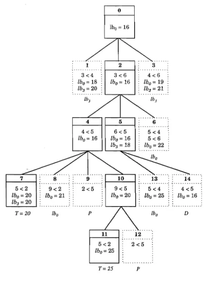
The search tree of the example is given in Fig. 7. The nodes contain several labels, indicating the node number, the added precedence constraints, the applicable lower bounds and the obtained upper bound (for the nodes representing a feasible solution). All fathomed nodes are

indicated by dashed lines. The reason for fathoming is indicated below the nodes: P (Precedence)

means the node represents a time-infeasible network; lbo means that lbo 2 T; lb3 means that

lbl ;;:: T and D means that the node was dominated. T = x means that a feasible solution with a makespan of x was found.

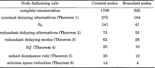
The number of nodes in the search tree (including dominated nodes, but apart from the root node) is equal to 14. The nodes actually branched from equals 4. Table II shows the impact of the node fathoming rules on the number of nodes created and branched from for the example. Notice, however, that the node fathoming rules in Table II are entered into the procedure in a sequential manner. Therefore, Table II does not reveal the power of each of the node fathoming rules. Estimating the impact of each of the node fathoming rules requires a full factorial experiment, in which all the combinations of the node fathoming rules are examined. This will be discussed in section 5. The resource profile of the optimal solution with respect to the first resource type is given in Fig. 8.

Table II. The impact of the node fathoming rules

Node fathoming rule Created nodes Branched nodes

complete enumeration 1709 325

minimal delaying alternatives (Theorem 1) 375 104

lbo 141 41

redundant delaying alternatives (Theorem 2) 73 33

redundant delaying modes (Theorem 3) 62 28

lbl (Theorem 4) 25 10

subset dominance rule (Theorem 5) 25 10

7 5<2 Lbo = 20 lb3 = 20 T=20 ---_._.-._--9<2 Lbo = 21 ---.---Lbo 1 3<4 Lbo = 18 lb3 = 20 4<5 Lbo = 16 --.--- _.---9 ---._._._. 2<5 .. _---P o Ibo = 16 2 3<6 Lbo = 16 6<5 Lbo = 16 lb3 = 18 9<5 lbo

=

20 3 _ .. ---4<6 Lbo = 19 lb3 = 21 5<4 5<6 Lbo = 22 13 ~ . ---. -. -. -5 <4 Lbo = 25 ---_ .. _----Lbo 1---="---1 ; ... : 5<2 Lbo = 25 2<5 : ' - -_ _ ...J ... . T= 25 P 14 ---.--.---4<5 Lbo = 16 ---_ .. _-D

Figure 7. The search tree for the example

Usage of resource type 1

10 --t:-=-,..."-,=-=---,, 9 8 7 6 5 4 3 2 1 1 2 3 4 5 6 7 8 9 10 11 12 13 14 15 16 17 18 19 20

Figure 8. The optimal resource profile of resource type 1

4.5. Another example

The following example (Demeulemeester, 1992) is a multi-project scheduling problem, in which three separate projects, each with a release date and a deadline, have to be scheduled, while subject to time-varying resource constraints. Fig. 9 clearly displays the three projects, which are connected to the dummy start and end activities such that one single project is obtained. The numbers above the nodes indicate the activity durations, the numbers below each node indicate the resource requirements for two renewable resources. The project is given in standardized form, so that the time lag values are all minimal start-start precedence relations. Notice that the time lags between activity 1 and activities 2, 7 and 11 (start-start lag of zero), and between activities 6, 10 and 13 and activity 14 (start-start lag equal to the duration of the predecessor activity) are needed to ensure that the (dummy) start and finish activities 1 and 14 correspond with the start and completion of the project. The release dates and deadlines are given in Table III. The resource availabilities vary over time as indicated in Table IV.

3 5

Figure 9. A multi-project GRCPSP

Table III. Release dates and deadlines for the three projects

Project Activities Release date Deadline

1 2, 3, 4, 5, 6 5 20

2 7,8,9,10 0 15